Abstract—A transient phase field model is developed of droplets and bubbles in viscous fluids subject to an external electric field. The model is transient and fully three-dimensional. It is based on the explicit finite difference solution, enhanced by parallel computing, of the coupled nonlinear governing equations for the electric field, the fluid flow field and free surface deformation. The effect of mesh size and interfacial thickness on numerical accuracy and stability of the phase field modeling is studied. The phase field model is validated with the Taylor theory for the deformation of a single dielectric droplet in electric fields. Computed results show that the deformation of a leaky dielectric droplet undergoes various different deformation stages before reaching the equilibrium oblate shape, which is caused by the free charge relaxation near the fluid-fluid interface. Also, the deformation and rising speed of the bubble are affected by the applied electric field in both magnitude and direction. For a rising bubble in a horizontal electric field, it rises slowly as a result of a larger drag caused by electric-stretching along the horizontal electric field. In comparison with the vertical field, the indentation on the bubble base starts earlier but grows more slowly after an initial period. The bubble deformation and fluid flow structure in a horizontal field are three dimensional.
Index Terms—phase field method, leaky dielectric model, electrohydrodynamics, two phase flow, fully 3D modeling
I. INTRODUCTION
nderstanding of the behavior of bubbles and droplets in electric fields is of great importance to a wide range of electrically-assisted thermal fluids systems. Studies on the behavior of fluids as affected by an external electric field, which falls into the category of electrohydrdynamics, started with Gilbert [1] in the 17th century, who observed the conical shape upon placing a charged rod above a sessile drop. This was followed by the work of Lord Rayleigh [2] on the deformation and the bursting of charged drops in electric fields. A poorly conducting liquid droplet in an electric field is known now to be better described within the framework of the leaky dielectrics [3], [4]. Over the last decade, there has
Manuscript received March 10, 2013; revised April 15, 2013. This work is supported by NSFC (Grant no. 90923040) and the National Basic Research Program of China (Grant no. 2009CB724202).
Q. Yang is with the State Key Laboratory for Manufacturing Systems Engineering, Xi’an Jiaotong University, Xi’an, Shaanxi 710049, P. R. China. He is currently a visiting PH.D. student in University of Michigan-Dearborn. (e-mail: [email protected])
B. Q. Li is with Department of Mechanical Engineering, University of Michigan, Dearborn, Michigan 48128, USA (corresponding author to provide phone: 313-593-5241; e-mail: [email protected]).
Y. Ding is with the State Key Laboratory for Manufacturing Systems Engineering, Xi’an Jiaotong University, Xi’an, Shaanxi 710049, P. R. China (e-mail: [email protected]).
been considerable interest in the EHD flows because of its wide spread industrial applications, such as coating flows [5], transport of small liquid samples in microfluidics [6], various applications that use the concept of the lab-on-a-chip [7] and pattern formation in soft lithography [8]-[11].
As with other complex flow problems, only a limited number of the EHD flow problems within an idealized setting can be solved analytically. Numerical simulations often are required to obtain solutions for the flow systems involving two fluids with different properties. For these two phase flow problems, the presence of the free surface poses a numerical challenge, for which various methods have been developed. Some popular numerical solution schemes include the level set method [12], [13], the volume of fluid method [14]-[16], and the front tracking method [17]. The phase field method, which is based on the coarse-grain averaging concept from statistical mechanics, has recently emerged as a useful vehicle to study the two phase flow problems [18]-[20]. A salient feature of the phase field based approach lies in its treatment of a moving or free surface as a thin molecular diffuse layer, thereby enabling a nanoscaled description of the collective behavior of molecules within the interface layer. Thus, within the framework of the phase field modeling, a sharp fluid-fluid interface is represented by a narrow layer in which the fluids may mix. The tracking of the interface is realized by a conserved order parameter (or the phase field parameter) that varies continuously over the thin interfacial layer but otherwise mostly uniform in the bulk fluid phases [21].
Computational modeling of two phase flows in electric fields has been reported in literature. Feng [22] calculated the equilibrium shape of a leaky dielectric droplet in an electric field by employing the Galerkin finite element method, coupled with the spine-parameterization of free surface boundaries. The scheme may work well for a 2D problem, but extension of it to 3D can be rather challenging. Sherwood [23] presented a boundary integral approach to model the large deformation of a droplet with finite conductivity in a creeping flow field. The model is capable of describing the drop breakup caused by either the electric stress or the mechanical stress due to the fluid motion. The EHD two phase flows have been studied recently using the level set and volume of fluid methods [24], and a front tracking/finite volume method [25], the latter also including various electrical property models (leaky dielectric, perfect dielectric, constant charged model) for the fluids. Recently, a phase field model was developed [26] for the 2D axisymmetric EHD flows.
This paper presents a 3D phase field model for the EHD two phase flows involving bubbles or droplets in applied electric fields. While 2-D models have been used often, there appears to be little information available on 3D models based on the phase field approach for the EHD two phase flow
Qingzhen Yang, Ben Q. Li, and Yucheng Ding
Phase Field Modeling of Drops and Bubbles in
Electric Fields
problems. The need for a 3D model cannot be overemphasized, because many electrically-assisted thermal fluids systems are fully three-dimensional. For example, an EHD patterning process recently developed for top-down nanofabrication of functional nanostructures involves the evolving free surfaces that are complex and three-dimensional in nature [11], [27]. Other cases such as the electro-coalescence of multiple droplets would also call for a full 3D representation. In what follows, the mathematical formulation and numerical development of the phase field model for the 3D EHD flows of leaky dielectric fluids are described. The computed results of 3D EHD two flows are selected from the examples of a deforming liquid drop and a rising bubble in electric fields.
II. MATHEMATICAL FORMULATIONS A. Phase field equations
In phase field description, the free energy density is represented by the phase parameter C, and the form of energy f : [0, 1] →R is taken as
( ) 1 2 1 1 2(1 )2
2 4
f C = ξγα∇C + ξ γα− C −C , ΩT : =Ω ×(0,T) (1)
where Ω is a bounded domain in R3, with a Lipschitz boundary ∂Ω, and C is the phase parameter, with the values of C=1 and C=0 corresponding to the two distinctive phases. Also, in the above equation, γ stands for surface tension, ξ measures the interface thickness and α=6 2 is a constant [28]. The first term in (1) accounts for the excess free energy due to the inhomogeneous distribution of the volume fraction in the interface region, whereas the second term represents the bulk energy density [29].
The Cahn-Hilliard equation with convection is employed here to describe the evolution of the phase field parameter C [20],
( ) 0
C
u C M
t φ
∂ + ⋅∇ − ∇ ⋅ ∇ =
∂ , ΩT (2)
where u represents the fluid velocity, φ = δf/δC the chemical potential, and M the phase field mobility.
B. Electric field equations
Within the framework of electrohydrodynamics, the Poisson equation may be used to describe the electric field distribution,
( )
(
0)
e
r C V
ε ε ρ
∇ ⋅ ∇ = − ΩT (3)
where ε0 is the permittivity of vacuum, εr(C) the dielectric constant, V the electric potential, and ρe the free charge density.
The free charge conservation can be expressed as [30],
( )
(
)
e
e
u C E
t
ρ ρ σ
∂
+ ⋅ ∇ = −∇ ⋅ ∂
Ω
T (4)
whereσ denotes the electrical conductivity, and E= −∇V is the electric strength. The second term on the left represents the transport of the free charges by convection, the term on the right stands for the transport by electromigration and the diffusion effect is neglected here [30].
Two limiting cases of (4) may be considered. First, if the time scale of charge relaxation tσ =ε ε σ0 r is much smaller than the time scale of the flow tc = Lc/Uc (Lc being the length scale, and Uc the characteristic velocity), then (4) reduces to
( )
(
σ C V)
0∇ ⋅ ∇ = ΩT (5)
Second, for poorly conductive materials, tσ>>tc. Thus, the free
charge may be neglected and a pure dielectric model is sufficient to describe the electric field [25], [26]. For this limiting case, (4) becomes redundant, and (3) recovers to the Laplace equation.
C. Fluid flow equations
The flow field is described by the governing equations of mass and momentum conservation with momentum sources from the electric field and interfacial energy. Both phases are considered to be incompressible. Hence the mass conservation over the whole simulation domain, including both fluid phases and their interface, can be expressed as [28],
0
u
∇⋅ =
ΩT (6)In the EHD system, the electric force and the surface tension force on the interface should be added. The modified Navier-Stokes equation for variable density and viscosity can be written as
( )C u ( )C u
( )
u +fe ft γ
ρ ∂ +ρ ⋅∇ = ∇ ⋅ Π +
∂
ΩT (7)
where the stress tensor П, the electric force fe
due to the polarization charge and free charge, and the surface tension force fγ
are given by the following expressions,
( )
(
)
,
T i j
pδ µ C u u
Π = − + ∇ + ∇ (8)
( )
2 2
0 0 , 0
1 1
2 2
e
e i j r
f = ∇ ⋅ε E⊗ −E ε Eδ =ρ E− ε E ∇ε C
(9)
fγ = ∇φ c
(10)
In (7) - (10), ρ(C) represents the density of fluid, p the pressure, μ the viscosity, and φ the chemical potential. D. Nondimensionalization
The governing equations above may be nondimensionalized with the characteristic length Lc, the velocity Uc, and the time tc= Lc/Uc. Uc is determined by balancing the electrical force and viscous force, Uc=ε0E02Lc/µ [30]. The nondimensionalization process produces the following dimensionless systems parameters,
0 0 c c U L Re ρ µ
= , Ca µ0Uc
γ
= , Pe L Uc c
M ξ γ = , c Cn L ξ
= , 0 r 02 c E
E L
Bo ε ε
γ
= (11) The well-known Reynolds (Re) number describes the relative importance between the inertial and the viscous forces. The Capillary (Ca) number measures the relative magnitude of the viscous force over the interface tension force. The Peclet (Pe) number is the ratio of the convective and diffusive mass transport. The Cahn number, Cn, defines the ratio between the interface thickness over the characteristic length. The electrical Bond number (BoE) describes the ratio of the electric over the surface tension effect. The density, electrical permittivity, conductivity, and viscosity ratios of the two fluids are defined as λρ = ρ1/ρ2, λε = ε1/ε2, λσ = σ1/σ2 and λµ =
µ1/µ2, respectively.
E. Numerical method
After discretization, the Poisson equation (3) can be written in the form Ax=b, where A coefficient matrix, x the unknown, b the force vector, and is solved by the successive over-relaxation (SOR) method. The iteration follows the scheme: x(k+1)=(D+ωL)-1{ωb-[ωU+(ω-1)D]x(k)}, where D, L and U are the diagonal, lower and upper triangular sub-matrices decomposed from matrix A. To speed up the rate of convergence, the relaxation coefficient is set at ω>1. The Navier-Stokes equation (7) is solved by the standard projection method [31], where the resulting Poisson equation is solved also by the SOR method. The forth order finite difference scheme is employed to solve the Cahn-Hilliard equation (2). It worth noting that the material parameters εr(C), σ(C), ρ(C), and μ(C)may be taken as a linear function of phase parameter C within the interface region. Numerical experience suggests, however, that the harmonic interpolation gives a better, more consistent approximation, when a large difference in density across the interface exists [21],
1 2 1
1 1 1 1
= 2
i i i
ρ+ ρ ρ+
+
1 2
(
1)
1 2
i i i
µ+ = µ µ+ + (12)
III. RESULTS AND DISCUSSION A. Computational details
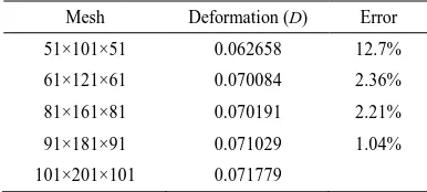
Before the numerical results are presented, computational aspects concerning the numerical accuracy warrant some discussion. Here, the mesh sensitivity is considered first, for the purpose of which the case of the single leaky droplet deformation under the influence of the electric field is chosen. The electric field configuration and the computational domain are shown in Fig. 1. For the droplet of radius R, a domain of (6R×6R×6R) is chosen for computation. Since the deformation is symmetric about the planes of x=0 and z=0, a 1/4 of the domain is needed (see Fig. 1b). For this problem, Lc=R. Other parameters for computations are: Re=1, Ca=0.2, Pe=1800, Cn=0.025, BoE=0.2, λρ=1, λε=2 and λµ=1. The computed results are listed in Table I for various meshes. For a coarse mesh, the computed results show the mesh-dependence. Progressive mesh refinement improves the
numerical accuracy. As evident from Table I, a mesh of 81×161×81 gives a reasonably good accuracy, which is thus used for the computations discussed below. Studies suggested that a spontaneous shrinkage of the drop occurs if the mesh is too coarse or the interface is too thick [33], [34]. This is also observed with the simulations in the present study. For the given parameters, with Cn=0.025 and a mesh of 81×161×81, the problem of artificial droplet shrinkage will not occur.
The Cahn number Cn=ξ/Lc is the ratio of the interface thickness over the characteristic length, which for the present studies is the size of the droplet or bubble. Fig. 2 compares the results obtained for the cases of Cn = 0.025 and Cn = 0.05. A mesh of 81×161×81 was used. For Cn=0.025, the mesh corresponds to the interface cell width ξ/min{Δx, Δy, Δz}=0.67 and good results were obtained. For the case of Cn=0.05, the flow pattern inside the droplet changes from the anticlockwise to clockwise rotation. This is because the flow vortex forms to satisfy mass conservation in a thicker interface and the sharp interface assumption of the phase field model breaks down. It is noted that the interface thickness is a physical property of the fluid-fluid interface, which is obtained either by molecular simulations [35] or by experiments. These results in Fig. 2 suggest that for the phase field model to be valid, the droplet size needs to be sufficiently large in comparison with the thickness of the interface.
B. Deformation of a single droplet (model validation) According to Taylor [4], if a droplet and its surrounding fluid are both leaky dielectrics, the droplet may deform into either a prolate or an oblate ellipsoid in a DC electric field. For the configuration shown in Fig. 1, an analytical expression can be obtained for the deformation of the droplet by the electric forces [4], [24]-[26],
( )
( )
1 2 1 2 1 2
2
1 2
/ , / , /
9
16 2 /
d E f
L B Bo
D
L B
σ σ ε ε µ µ σ σ
−
= =
+ + (13)
[image:3.595.56.281.59.134.2]where L and B are the lengths of the axes of the ellipsoid parallel and perpendicular to the applied electric field, and the Fig. 1. Schematic illustration of an EHD two phase flow problem: (a) a
droplet in an electric field generated by two electrodes and (b) the computational domain.
TABLE I.
THE MESH SENSITIVITY OF LEAKY DROPLET DEFORMATION*
Mesh Deformation (D) Error
51×101×51 0.062658 12.7%
61×121×61 0.070084 2.36%
81×161×81 0.070191 2.21%
91×181×91 0.071029 1.04%
101×201×101 0.071779
* The case 101×201×101 is used as a base for comparison
[image:3.595.336.529.77.164.2]subscripts 1 and 2 denote the droplet and the surrounding host fluid, respectively. The dimensionless parameters in (11) are scaled by the properties of the fluid 2, with Lc = R, the radius of the sphere. The function, fd
(
σ σ ε ε µ µ1/ 2, 1/ 2, 1/ 2)
, is the discriminating function,( )
( )
2
1 2
1 1 1 1 1 1 1
2 2 2 2 2 2 2 1 2
2 3 3
, , 1 2
5 1
d
f σ ε µ σ ε σ ε µ µ
σ ε µ σ ε σ ε µ µ
+
= + − + −
+
(14) by which the droplet takes a spherical shape for fd=0, a prolate shape for fd <0 and an oblate shape for fd >0.
The computational domain consists of a cube Ω = [0,l ]x [0,l ]x[0,l ] and the boundary conditions are the same as in [26], the difference being that here the 3D calculations are considered. Symmetric conditions are applied on the z=l/2 and x=l/2 planes and as such only a quarter of the domain needs to be discretized. The boundary conditions are listed as follows,
0
V=V u=0 ∈ ∂Ω = ×{ y l}
( )
0,T( )
0 0 { 0} 0,
V= u= ∈ ∂Ω = ×y T
( )
0 0 { 0 0 } 0,
2 2
V l l
u n x x z z T
n
∂ = = ∈ ∂Ω = ∪ = ∪ = ∪ = ×
∂
( )
0 0 0 0,
p C
T
n n n
φ
∂ = ∂ = ∂ = ∈∂Ω×
∂ ∂ ∂
[image:4.595.80.252.56.191.2]where ∂Ω is the boundary of computational domain. Initially the velocity is set to zero and the phase field is C=1 for the droplet and C=0 elsewhere. The discretized mesh used for calculations below was 81x161x81. The original radius of the droplet R=l/6, and it is also used as the characteristic length. The parameters used for the calculations are: Re=1, Ca=0.2, Pe=1800, Cn=0.025, BoE=0.2, λρ=1, λε=2, λµ=1 and l = 6R.
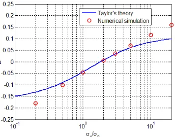
Fig. 3 compares the results obtained from the present 3D phase field calculations and from the analytical solution (13). As it is seen, for small deformations, the 3D numerical and the
analytical solutions match very well. For large deformations, however, the numerical model deviates from the analytical solution. This is expected in that (13) is based on the linear perturbation analysis, which is valid only for small droplet deformations.
C. Transient Behavior of Electrically-induced Droplet Deformation
While the analytical solution is for a steady state deformation, the phase field model is fully 3D and transient, which allows us to capture the transient behavior of a droplet as it undergoes deformation. Information on the transient development of droplet deformation is of critical value in analyzing the underlying physics governing the electrohydrodynamics of a deforming droplet. One interesting case is presented in Fig. 4, where the final (or equilibrium) droplet shape is oblate. The droplet deformation for this case undergoes several different phases as the droplet deformation transits in time to reach the equilibrium from its initial condition. The transient development of the deformation experiences the follow stages: it starts with a spherical shape, evolves to a prolate ellipsoid, returns to spherical, and finally becomes oblate. The detailed flow velocity field, flow streamlines, droplet deformation and phase field are also plotted in Fig. 4 for three different droplet deformation stages. Detailed analysis of the simulation data reveals that this transition in deformed shapes is a result of electric charge interacting with the fluid flow field. At the onset of the deformation process, there is no free charge and, the whole system behaves like pure dielectric materials. The droplet deformation is dominated by the dielectric forces, which leads to a prolate ellipsoidal shape. This has been shown by both experimental measurements and theoretical analyses [24], [25]. As the time goes by, free charges start to accumulate at the droplet-fluid interface as demanded by (4), and the additional Coulomb force gradually comes into play, which acts to compress the droplet along the two poles. As a result, the droplet returns to a spherical shape, and then evolves continuously and eventually into the final oblate shape. It is important to stress that the transition will not occur if (5) were used to model the free charge distribution. This is because by (5) the free charge distribution is assumed to be established instantaneously and no charge relaxation will occur.
D. Bubble deformation in electric fields
The 3D phase field also can be applied to study the deformation behavior of a bubble in an electric field with a change of appropriate parameters. Simulations were carried Fig. 3. Comparison of the deformation D between the analytical solutions
and the 3D phase field numerical results for BoE=0.2, λε=ε1/ε2=2 and
λµ=µ1/µ2=1.
Fig. 4. Transient development of droplet deformation, where the cross section at z=0 is shown rather the 3D shape along with the fluid flow field and phase field. The initially spherical shape is spherical (not shown). The deformation undergoes through the prolate first (a), then the spherical (b), and then eventually the oblate shape (c). The dimensionless time for (a-c) are t*=1.8, 8.46 and 360, respectively. The corresponding deformation parameters
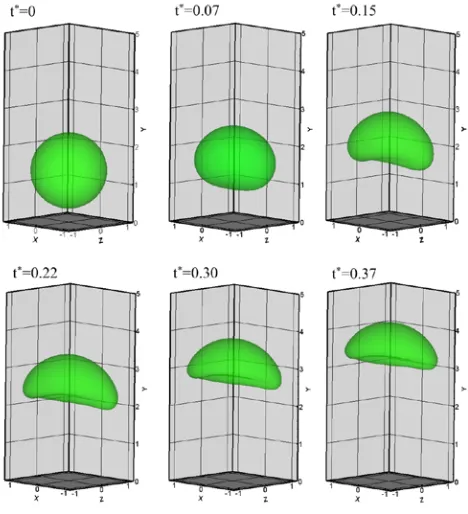
[image:4.595.130.469.616.731.2]out for various conditions. Fig. 6 shows the dynamic development of a bubble as it rises up through a viscous fluid subject to a horizontal electric field (i.e. the electric field imposed in the x-direction). For this case, the electrical Bond number BoE=2.3 was chosen. Other parameters are Re=1, Ca=0.76, Pe=1.1, Cn=0.025, λρ=10-3, λε=1/3 and λµ=1/80. Electrical conductivity is not considered in this case. The bubble is seen to start rising up from the stationary with the initial shape of a sphere. While ascending upwards, it is being stretched out in the x direction by the applied electric force. The bubble deformation and fluid regime in this case are not axisymmetric anymore and the 3D model is required to simulate the process. Eventually the bubble evolves into a complex 3D shape as shown in Fig. 5. The deformation of the bubble and the fluid flow are viewed from different angels in Fig. 6. Other characters are also observed, such as the occurrence of indentation at the bottom and the deformation of the bubble into an oblate ellipsoidal cap eventually.
Computations were also carried out for a rising bubble in a vertical electric field, in which case the bubble deforms into a prolate ellipsoid. Different from the case with a vertical electric field, the bubble with a horizontal electric field deforms into an oblate ellipsoid directly. Since the horizontal electric field tends to stretch the bubble into an oblate shape, it contributes to the formation of the indentation. Additional
results show that the indentation occurs earlier than the case without an electric field. This is because it is easier for indentation to occur on an oblate than a prolate ellipsoid. In a longer time duration, however, the horizontal electric field impedes the further development of indentation. In the horizontal electric field, the bubble rises more slowly due to the high resistant drag force; meanwhile the jet flow underneath the bubble is weakened. As pointed out before, the development of indentation is caused by the jet flow, and the weak jet flow in turn leads to a slower indentation development.
IV. CONCLUSIONS
This paper has presented a phase field computational methodology for the numerical solution of 3D electrohydrodynamic two phase flow problems involving liquid drops or gas bubbles in electric fields. The mathematical formulation consists of a set of coupled nonlinear equations, including the Navier-Stokes equations for fluid motion, the convective Cahn-Hilliard equation for the phase field, and the charge conservation equation for the electric field distribution in pure and/or leaky dielectric fluids. These equations are discretized by the finite difference method along with the explicit time matching scheme, enhanced by parallel computing. The 3D model is validated by comparing with the Taylor model for a droplet deformation in an electric field. It is found that while a leaky dielectric droplet deforms into an oblate ellipsoid as its final equilibrium shape in an electric field, the transient development in deformation entails the transition from the initial spherical to the prolate and then to the intermediate spherical and eventually the final oblate shape. For a rising bubble in an electric field, its ascending speed slows down as a result of stretching by the electric forces along the horizontal electric field. Compared with the vertical field, the indentation on the bubble base starts earlier but grows more slowly after an initial period. The bubble deformation and fluid flow structure in a horizontal field are three dimensional.
REFERENCES
[1] W. Gilbert, “de Magnete” (Dover, New York, 1958), Vol. II, Chap. II, pp. 89, first published ca. 1600, translated by P. F. Mottelay in 1893. [2] L. Rayleigh, “On the equilibrium of liquid conducting masses charged
with electricity,” Phil. Mag. Ser., vol. 14, pp. 184–186, 1882. [3] R. S. Allan and S. G. Mason, “Particle behavior in shear and electric
fields. I. Deformation and burst of fluid drops,” Proc. R. Soc. A, vol. 267, pp. 45–61, 1962.
[4] G. Taylor, “Studies in Electrohydrodynamics. I. The Circulation Produced in a Drop by Electrical Field,” Proc Roy. Soc. Lond. Ser. A: Math. Phys. Sci., vol. 291, pp. 159-166, 1966.
[5] R. J. Fermin, “Electrohydrodynamic coating flows,” Ph.D. thesis, University of Minnesota, 2001.
[6] H. A. Stone, A. D. Stroock and A. Ajdari, “Engineering flows in small devices: Microfluidics toward a lab-on-a-chip,” Annu. Rev. Fluid Mech., vol. 36, pp. 381–411, 2004.
[7] J. Zeng, T. Korsmeyer, “Principles of droplet electrohydrodynamics for lab-on-a-chip,” Lab Chip, vol. 4, pp. 265–277, 2004.
[8] S. Y. Chou, L. Zhuang and L. Guo, “Lithographically induced self-construction of polymer microstructures for resistless patterning,” Appl. Phys. Lett., vol. 75, pp. 1004–1006, 1999.
[9] S. Y. Chou and L. Zhuang, “Lithographically induced self-assembly of periodic polymer micropillar arrays,” J. Vac. Sci. Technol. B, vol. 17, pp. 3197–3202, 1999.
[image:5.595.55.289.62.319.2][10] E. Schaffer, T. Thurn-Albrecht, T. P. Russell and U. Steiner, “Electrically induced structure formation and pattern transfer,” Nature (London), vol. 403, pp. 874–877, 2000.
Fig. 5. Bubble deformation in a horizontal electric field.
[image:5.595.54.290.354.448.2][11] N. Wu, W. B. Russel, “Micro- and nano- patterns created via electrohydrodynamic instabilities,” Nano Today, vol. 4, pp. 180–192, 2009.
[12] D. Adalsteinsson and J. Sethian, “A fast level set method for propagating interfaces,” J. Comput. Phys., vol. 118, pp. 269–277, 1995,
[13] M. Sussman, P. Smereka and S. Osher, “A level set approach for computing solutions to incompressible two-phase flow,” J. Comput. Phys., vol. 114, pp. 146–159, 1994.
[14] C. W. Hirt, B. D. Nichols, “Volume of fluid (VOF) method for the dynamics of free boundaries,” J. Comput. Phys., vol. 39, pp. 201–225, 1981.
[15] B. D. Nichols, C. W. Hirt and R. S. Hotchkiss, “SOLA-VOF: A solution algorithm for transient fluid flow with multiple free boundaries,” Los Alamos National Lab Report LA-8355, 1980. [16] E. G. Puckett, A. S. Almgren, J. B. Bell, D. L. Marcus and W. J. Rider,
“A high-order projection method for tracking fluid interfaces in variable density incompressible flows,” J. Comput. Phys., vol. 130, pp. 269–282, 1997.
[17] G. Tryggvason, B. Bunner, A. Esmaeeli, D. Juric, N. Al-Rawahi, W. Tauber, J. Han, S. Nas and Y.-J. Jan, “A front-tracking method for the computations of multiphase flow,” J. Comput. Phys., vol. 169, pp. 708–759, 2001.
[18] D. M. Anderson, G. B. McFadden and A. A. Wheeler, “Diffuse-interface methods in fluid mechanics,” Ann. Rev. Fluid Mech., Vol. 30, pp. 139–165, 1998.
[19] V. E. Badalassi, H. D. Ceniceros and S. Banerjee, “Computation of multiphase systems with phase field models,” J. Comput. Phys., vol. 190, pp. 371–397, 2003.
[20] D. Jacqmin, “Calculation of two-phase Navier-Stokes flows using phase-field modeling,” J. Comput. Phys., vol. 155, pp. 96–127, 1999. [21] J. Kim, “Phase-Field Models for Multi-Component Fluid Flows,”
Commun. Comput. Phys., vol. 12, pp. 613–661, 2012.
[22] J. Q. Feng and T. C. Scott, “A computational analysis of electrohydrodynamics of a leaky dielectric drop in an electric field,” J Fluid Mech., vol. 311, pp. 289–326, 1996.
[23] J. D. Sherwood, “Breakup of fluid droplets in electric and magnetic fields,” J. Fluid Mech., vol. 188, pp. 133–146, 1988.
[24] G. Tomar, D. Gerlach, G. Biswas, N. Alleborn, A. Sharma, F. Durst, S.W. J. Welch and A. Delgado, “Two-phase electrohydrodynamic simulations using a volume-of-fluid approach,” J. Comput. Phys., vol. 227, pp. 1267–1285, 2007.
[25] J. Hua, L. K. Lim, C.-H. Wang, “Numerical simulation of deformation/motion of a droplet suspended in viscous liquids under influence of steady electric field,” Phys. Fluid, vol. 20, pp. 11302–11317, 2008.
[26] Y. Lin, P. Skjetne and A. Carlson, “A phase field model for multiphase electro-hydrodynamic flow,” Int. J. Multiphase Flow, vol. 45, pp. 1–11, 2012.
[27] Q. Yang, B. Q. Li, Y. Ding, “A numerical study of nanoscale electrohydrodynamic patterning in a liquid film,” Soft Matter, vol. 9, pp. 3412-3423, 2013.
[28] H. Ding, P. D. M. Spelt and C. Shu, “Diffuse interface model for incompressible two-phase flows with large density ratios,” J. Comput. Phys., vol. 226, pp. 2078–2095, 2007.
[29] J. W. Cahn and J. E. Hilliard, “Free energy of a nonuniform system. I. Interfacial Free Energy,” J. Chem. Phys., vol. 28, pp. 258–267, 1958. [30] D. A. Saville, “Electrohydrodynamics: The Taylor-Melcher Leaky
Dielectric Model,” Annu. Rev. Fluid Mech., vol. 29, pp. 27–64, 1997. [31] O. Zikanov, “Essential Computational Fluid Dynamics,” John Wiley &
Sons, 2010,
[32] H. Johnston, J.-G. Liu, “Finite Difference Schemes for Incompressible Flow Based on Local Pressure Boundary Conditions,” J. Comput. Phys., vol. 180, pp. 120–154, 2002.
[33] P. Yue, C. Zhou and J. J. Feng, “Spontaneous shrinkage of drops and mass conservation in phase-field simulations,” J. Comp. Phys., vol. 223, pp. 1–9, 2007
[34] A. A. Donaldson, D. M. Kirpalani and A. Macchi, “Diffuse interface tracking of immiscible fluids: Improving phase continuity through free energy density selection,” Int. J. Multiphase Flow, vol. 37, pp. 777–787, 2011.