Sound Propagation and Reconstruction Algorithm Based on Geometry

(1)

Sound Propagation and Reconstruction Algorithm

Based on Geometry

https://doi.org/10.3991/ijoe.v15i13.11212

Jihun Park

Hongik University, Seoul, S. Korea [email protected]

Abstract—This paper presents a method of simulating sound propagation and reconstruction for the virtual reality applications. The algorithm being developed in this paper is based on a ray sound theory. If we are given 3 dimensional geom-etry input as well as sound sources as inputs, we can compute sound effects over the entire boundary surfaces. In this paper, we present two approaches to compute sound field: The first approach, called forward tracing, traces sounds emanating from sound sources, while the second approach, called geometry based compu-tation, computes possible propagation routes between sources and receivers. We compare two approaches and propose a geometry-based sound computation method for outdoor simulation. This approach is computationally more efficient than the forward sound tracing. The physical environment affects sound propa-gation simulation by impulse- response. When a sound source waveform and nu-merically computed impulse in time is convoluted, a synthetic sound is generated. This technique can be easily generalized to synthesize realistic stereo sounds for the virtual reality applications. At the same time, the simulation result can be visualized using VRML.

Keywords—Sound propagation, simulation, vrml, forward tracing, geometry

1 Introduction

(2)

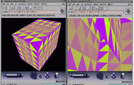
Fig. 2. Forward tracing.

When sound is transmitted, refraction, reflection and diffraction phenomenon is ex-hibited whenever the medium with different density is encountered. In this paper, the approach taken is to calculate geometrical relation between sound source and receiver, and calculate direct and indirect sound propagation. We constructed three-dimensional terrain using fractal geometry, and developed an algorithm for sound propagation sim-ulation for outdoor terrains and indoor rooms. The above three-dimensional model can be easily replaced by standard input files, for example, AutoCAD's dxf or dwg files. But the above available three-dimensional model files require further work to triangu-late a big polygon into small triangles for setting receivers on the model surfaces. Figure 1 shows a fractal-generated terrain, and the size of each triangle constituting the terrain shown can be easily adjusted. We had generated two different kinds of terrains: flat and wavy. For the two kinds of terrains in figure 1, we performed simulations using two different algorithms: forward tracing from sound source, and geometry-based compu-tation.

Although the simulation time by the forward sound tracing can be short if a fixed number of sound vectors are cast, surface triangles will often be missed by the cast vectors, resulting in poor simulation quality. We need extra control in the number of tracing vectors cast by considering the distance between sound source and terrain sur-faces. In order to improve the simulation quality, we have to incur additional time. The inverse direction tracing method is tracing sound from sound receivers to sources.

(3)

2 Related Research

The electric wave and sound have very close relationship. We wish to distinguish the sound and electric wave by frequency band. In noise and vibration theory, sound is usually traced in forward direction from a sound source. According to this method, computation time may be wasted because tracing sound vector, which is not useful, or may result in poor simulation result due to omitted surface computation. This kind of computer-based ray tracing approach can be found in papers dealing with electric wave propagation.

Owing to very close relationship, we found several related papers dealing with com-puter-based electromagnetic wave simulation. Paper [1] computes direct and single re-flection wave propagation; multiple rere-flection propagation cannot be handled, however. For multiple reflection computation, ray-tracing based approach is more appropriate. Papers [2,3] uses three-dimensional ray tracing method for single source and single receiver. We have a solution of multiple sources and receivers, but the computation time is very long. Paper [4] uses a kind of ray tracing by dividing surfaces, and paper [5] deals with two-dimensional knife-edge diffraction. Our algorithm is similar to both ODEON [12] and RAYNOISE [13], but our main target is outdoor simulation.

3 Sound Tracing Algorithm

3.1 Sound tracing methods

Forward sound tracing algorithm

Forward Sound Tracing Algorithm( ) {

loop_1: a sphere representing a source is divided by n equal latitudinal angles

loop_2: a sphere representing a source is divided by 2n equal longitudinal angles

a center of an area on the sphere is computed; tracing_vector = center_of_area - sphere center; compute intersection between a tracing_vector and terrain triangles;

loop_2_end loop_1_end }

(4)

receiver. The backward tracing produces the best results but entails long computation time. The forward tracing can give quick but poor simulation results.

Because we are concerned with outdoor sound tracing simulation, we adopted ge-ometry-based approach. In outdoor environment, we can safely assume there occurs limited number of reflections. The backward tracing is too costly. But the forward trac-ing produces poor results if we cast small number of sound vectors, but casttrac-ing large number of vectors for better simulation result can be quite expensive.

3.2 Forward sound tracing

The forward tracing cast tracing vectors from sound sources. The cast vectors are traced using reflections. Figure 2 shows an overview of tracing sounds from a source to a receiver. Figure 3 shows forward tracing simulation results on fractal generated terrains, both flat and wavy. We assumed there is no transmission of sounds on outdoor terrain. A tracing vector is cast from a sound source. We traced the reflected vector whenever it hits a surface using the fact input angle is the same as the output angle. The power level of a tracing vector is diminished each time it is reflected. If the power of tracing vector becomes too weak, we quit tracing. The fractal generated terrain was modelled using triangles. We placed a receiver on each triangle. The position of receiver is given at the height of 1.5 meters at the center of each triangle. Each triangle has geometry information as well as surface reflection characteristics for each 8-octave frequency bands. The center frequency of each octave band was used for simulation. If there are several routes from a source to a receiver, then the power of all routes travelled are added to determine the sound pressure of the surface.

Vector intersection computation

compute_intersection (input is tracing_vector) {

Finds the nearest triangle; If not found then return;

Determine the intersected triangles and its intersec-tion posiintersec-tion;

Record intersection position and sound pressure as intersected triangle information;

Compute reflection vector;

Determine reflection vector sound pressure according to reflection coefficient;

Compute transmission vector;

Determine transmission vector sound pressure accord-ing to transmission coefficient;

(5)

Recursive function compute_intersection() gets each tracing vector as an input. The tracing vector is traced from a sound source, and whenever it hits a terrain triangle, the reflection vector is computed and tracing restarts from the triangle.

3.3 Propagation simulation by geometric computation

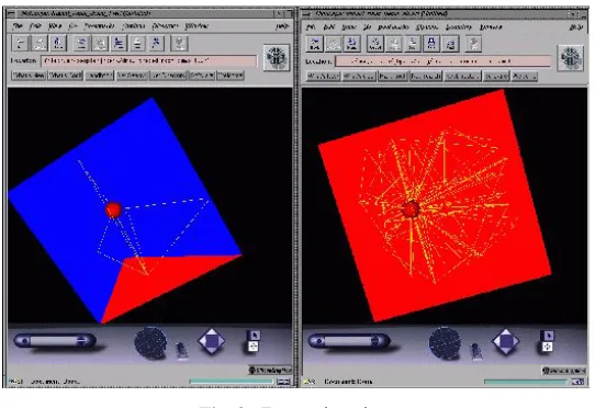
Fig. 3. Propagation computation based on geometry (1 reflection)

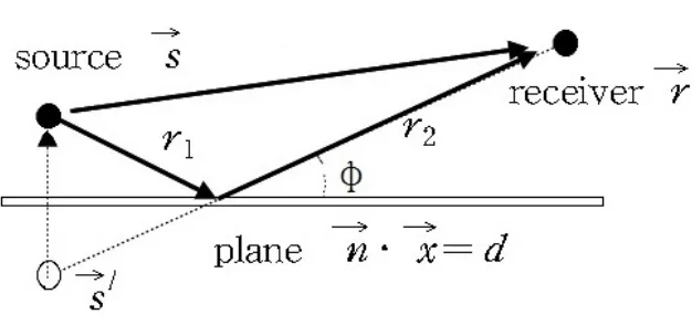
In order to improve the forward tracing simulation quality, long computational time is required. We developed a simulation by geometric reflection to shorten the compu-tational time, and adopted here. In this method, we assume there is limited number of sound reflections between sources and receivers. This assumption is acceptable for out-door environment. Figure 4 shows a single reflection sound propagation as well as a direct propagation. The major advantage of this approach is shorter computation time. Figure 5 shows simulation result by geometric reflection computation. This figure of-fers good comparison with figure 3. In figure 3, we can find many triangles whose sound pressure levels were not computed. But in figure 5, every surface triangle has the sound pressure level computed. The left figure on the left side is simulation result on flat terrain, while the figure on the right shows result on wavy terrain. Because we did not consider any diffraction, there are some triangles which have zero sound pressure levels. 𝑛"⃗ is a normal of a reflection surface, 𝑠⃗/_{is a position vector of a virtual sound}

source, 𝑛"⃗ ∙ 𝑥⃗ = d is a plane equation of a reflection surface. 𝑠⃗/_{= 𝑠⃗ + 2 (𝑑 − 𝑛"⃗ ∙ 𝑠⃗ )𝑛"⃗/}

(6)

Fig. 4. Propagation computation result of 1 reflection

The following shows a geometric simulation algorithm for n sound sources. In this algorithm, we assume that only single reflection is allowed.

Vector intersection computation

Geometric reflection computation( ) {

loop_1 : for every m terrain triangles loop_2 : for n sound sources

Compute the center of a triangle for loop_1 ; /* receiver computation */

Elevate by 1.5 meter on vertical direction from the center ;

Check Direct path from source to receiver ; If direct path exists, record the length of the path ;

/* check 1 reflection from source to receiver */ loop_3 : for m terrain triangles

Check for a path via triangle of loop_3 ; If exists, record the length of the path ; Compute sound pressure level and added on the existing value;

loop_3_end, loop_2_end, loop_1_end

(7)

3.4 Computing sound pressure level

The sound propagation is affected by many factors such as temperature, humidity, wind and reflection coefficient of the terrain. The most important factor is distance from a source to a receiver. We need to get accurate propagation computation. Whenever there is a sound propagation from a source to a receiver, there may be a direct propaga-tion. The length between a source and a receiver is denoted as R in figure 4. For indirect propagation, we can compute lengths 𝑟3 and 𝑟1. SPL is computed according to the

fol-lowing set of equations [9,10,11]. t is temperature in the Celsius, ρ6c is impedance

value of air, σ is flow resistivity, 𝑍9is an impedance of a reflection surface, 𝑅; is

re-flection coefficient, α is absorption coefficient, SPL is sound pressure level, W is sound power level, φ is angle between reflection vector and reflection surface, and f is central frequency of each octave band. ρ6= 1.24, c = 331+0.6t, 𝑍9= ρ6c (1+0.057(ρ6f/

σ)B6.6CD_{-i 0.087 (ρ}

6f/σ)B6.CE1), 𝑅;= (sin φ − ρ6c/𝑍9)/( sin φ + ρ6c/𝑍9), α = 1 −

I𝑅;I 1

, SPL = 20 log (SQRT(ρ6c W (1/𝑅;1+(1- α)/( 𝑟3+ 𝑟1)1)/(4𝜋))/(20×10BV)).

3.5 Sound tracing using frequency characteristics

The sound propagation characteristic of reflection coefficient and speed reduction rate depends on frequency. The sound tends to move straight in high frequency, which means that the sound moves directionally. But for low frequency sounds, diffraction effect occurs and the propagation is omni-directional. In this paper, we developed a program that computes the impedance for determining reflection coefficient. For each sound vector cast from the source, we simulate separately for each frequency band. This means we have eight different terrain impedances for each sound vector.

4 Conclusion

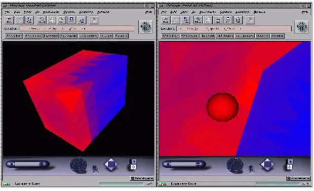
In this paper, we considered two different methods of tracing sounds. The forward tracing has the limitation of either low simulation quality or long computational time. These limitations are caused by incomplete modelling of sound sources. Although we can devise a better modelling method, it is not easy to compute in short time while improving simulation quality. Our proposed approach involves computing using geo-metric reflections. Although we limit the number of reflections, it is acceptable for out-door where only a limited number of reflections occur. Figure 5 shows simulation re-sults for input terrain given in Figure 1. For the red surface, our hearing is quite good, while the blue surface implies deteriorating in hearing. Figure 3, obviously of lower quality, shows simulation by the forward tracing method. This is why we choose to use geometric computation for outdoor sound simulation.

(8)

different/extra routes, which produce different simulation results. Our future research will be selecting proper triangle size in modelling of the environment.

5 Acknowledgement

This work was supported by 2018 Hongik University Research Fund.

6 References

[1] Ho, C. and Rappaport, T. (1993) Wireless channel prediction in a modern office building using an image-based ray tracing method, Proc. of the Globecom '93. https://doi.org/10.1109/glocom.1993.318274

[2] Reinaldo, A. and Valenzuela, A, (1993) Ray tracing approach to predicting indoor wireless transmission, Proc. of the 1993 IEEE 43th Vehicular Technology Conference. https://doi.org/10.1109/vetec.1993.507047

[3] Naruniranat, S., Huang, Y. and Parsons, D. (1999) A three-dimensional image ray tracing (3D-IRT) method for indoor wireless channel characterization, Proc. of the 1999 High Fre-quency Postgraduate Student Colloquium. https://doi.org/10.1109/hfpsc.1999.809281 [4] Zhang, Z., Yun, Z. and Iskander, M. (2000) Ray tracing method for propagation models in

wireless communication systems, Electronics Letters, 36 pp464. https://doi.org/10.1049/el:20000345

[5] Mokhtari, H. and Lazaridis, P. (1999) Comparative study of lateral profile knife-edge dif-fraction and ray tracing technique using GTD in urban environment, IEEE Transactions on Vehicular Technology, 48 pp255. https://doi.org/10.1109/25.740101

[6] Fapojuwo, A. et al (1992) A simulation study of speech traffic capacity in digital codeless telecommunication systems, IEEE Transactions on Vehicular Technology, 41 pp5. https://doi.org/10.1109/25.120140

[7] Kuttruff, H. (1991) Room Acoustics 3rd ed, Elseiver applied science.

[8] Watt, A. and Watt, M. (1992) Advanced Animation and Rendering Techniques: Theory and Practice, Addison-Wesley.

[9] Delany, M. and Bazley, E. (1970) Acoustical properties of fibrous absorbent materials, Ap-plied Acoustics, 3 pp105. https://doi.org/10.1016/0003-682x(70)90031-9

[10] Miki, Y. (1990) Acoustical properties of porous materials-modification of Delany Bazley models, J. Acoust. Soc. Japan 11 pp19.

[11] Embleton, T., Piercy, J. and Olson, N. (1976) Outdoors sound propagation over ground of finite impedance, Journal of Sound and Vibration, 59 pp267.

[12] ODEON, http://www.dat.dtu.dk/~odeon/OdSound1.htm.

[13] RAYNOISE, http://www.ingeciber.com/eng/products/default.htm.

7 Author

(9)

March 1988 to August 1993, he was an assistant professor in the Department of Com-puter Engineering at Pusan University of Foreign Studies, Pusan, Korea. In August 1994, he joined the faculty of the Department of Computer Engineering at Hongik Uni-versity, 94 Wowsanro, Mapo, Seoul, Korea, and he is now a full professor. His research interests include image processing and computer graphic animation.