Modeling the interaction of light with photonic structures by direct numerical solution of Maxwell'€™s equations

UNIVERSITA’ di TRENTO

Dipartimento di Fisica

Ph.D. degree in Physics

Modeling the interaction of light with photonic structures by

direct numerical solution of Maxwell’s equations

Candidate:

Alessandro Vaccari

Advisor:

Dott. Lucia Calliari

Fondazione Bruno Kessler

FBK-LISC

Contents

Introduction and motivation vii

I

Some selected topics in electromagnetism and wave

optics

1

1 Electromagnetism in matter 3

1.1 Maxwell’s equations in matter . . . 3

1.2 Temporally dispersive media. . . 6

1.3 Solution for the sphere in the field of a plane wave . . . 7

2 Spatial Fourier analysis and far-fields 15 2.1 Plane wave spectrum representation . . . 15

2.2 Far-field in the angular spectrum representation . . . 17

2.3 Kirchhoff formula and the near to far field transform . . . 18

3 Gaussian beams 23 3.1 Paraxial approximation . . . 23

3.2 Gaussian laser beams . . . 24

3.3 Focused beams . . . 25

4 Planarly multilayered media 31 4.1 Matrix method for R and T . . . 31

4.2 E~ and H~ field distributions . . . 39

4.3 The inverse transmittance problem . . . 41

4.4 Continuously varying refractive index . . . 43

II

Implementation of the FDTD numerical method 45

5.2 Stability . . . 55

5.3 Frequency domain analysis . . . 57

6 Absorbing boundary conditions 63 6.1 Convolutional-Perfectly Matched Layer . . . 64

6.2 Periodic boundary conditions . . . 81

7 Linearly polarized plane wave excitation 83 7.1 Propagation along a coordinate axis . . . 85

7.2 Propagation along arbitrary directions . . . 86

8 Algorithm modification for dispersive materials 87 8.1 Recursive convolution . . . 87

8.2 Auxiliary differential equation . . . 88

9 FDTD algorithm parallelization 93 9.1 Domain decomposition . . . 94

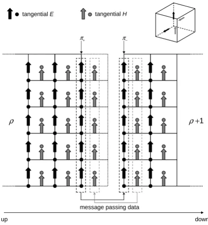
9.2 Suitable MPI data structures . . . 97

III

Applications of the FDTD method

101

10.2 Scalability of the parallelized code . . . 107

11 Plasmonics applications 111 11.1 Scattering from spherical nanoparticles. Analytical case. . . . 112

11.2 Scattering from nonspherical nanoparticles. FDTD case. . . . 118

11.3 Arrayed particles on a silicon substrate. . . 121

12 Photonics application to an opal crystal 133 12.1 Eigenvalue problem and the band structure . . . 134

12.2 The FCC opal photonic crystal . . . 136

12.3 Multilayer equivalence: homogenization . . . 147

12.4 Dispersion band structure reconstruction . . . 150

A Some dyadics calculations 155

B Some Gaussian integrals 157

CONTENTS v

Introduction and motivation

The present work analyzes and describes a method for the direct numeri-cal solution of the Maxwell’s equations of classinumeri-cal electromagnetism. This is the FDTD (Finite-Difference Time-Domain) method, along with its imple-mentation in an “in-house” computing code for large parallelized simulations. Both are then applied to the modelization of photonic and plasmonic struc-tures interacting with light. These systems are often too complex, either geometrically and materially, in order to be mathematically tractable and an exact analytic solution in closed form, or as a series expansion, cannot be obtained. The only way to gain insight on their physical behavior is thus to try to get a numerical approximated, although convergent, solution.

This is a current trend in modern physics because, apart from perturbative methods and asymptotic analysis, which represent, where applicable, the typ-ical instruments to deal with complex physico-mathemattyp-ical problems, the only general way to approach such problems is based on the direct approxi-mated numerical solution of the governing equations. Today this last choice is made possible through the enormous and widespread computational capabili-ties offered by modern computers, in particular High Performance Computing (HPC) done using parallel machines with a large number of CPUs working concurrently. Computer simulations are now a sort of virtual laboratories, which can be rapidly and costless setup to investigate various physical phe-nomena. Thus computational physics has become a sort of third way between the experimental and theoretical branches.

The plasmonics application of the present work concerns the scattering and absorption analysis from single and arrayed metal nanoparticles, when sur-face plasmons are excited by an impinging beam of light, to study the radi-ation distribution inside a silicon substrate behind them. This has potential applications in improving the efficiency of photovoltaic cells.

The photonics application of the present work concerns the analysis of the optical reflectance and transmittance properties of an opal crystal. This is a regular and ordered lattice of macroscopic particles which can stops light propagation in certain wavelenght bands, and whose study has potential

plications in the realization of low threshold laser, optical waveguides and sensors. For these latters, in fact, the crystal response is tuned to its struc-ture parameters and symmetry and varies by varying them.

The present work about the FDTD method represents an enhacement of a previous one made for my MSc Degree Thesis in Physics, which has also now geared toward the visible and neighboring parts of the electromagnetic spectrum. It is organized in the following fashion.

Part I provides an exposition of the basic concepts of electromagnetism which constitute the minimum, although partial, theoretical background useful to formulate the physics of the systems here analyzed or to be analyzed in pos-sible further developments of the work. It summarizes Maxwell’s equations in matter and the time domain description of temporally dispersive media. It addresses also the plane wave representation of an electromagnetic field distribution, mainly the far field one. The Kirchhoff formula is described and deduced, to calculate the angular radiation distribution around a scatterer. Gaussian beams in the paraxial approximation are also slightly treated, along with their focalization by means of an approximated diffraction formula use-ful for their numericall FDTD representation. Finally, a thorough descrip-tion of planarly multilayered media is included, which can play an important ancillary role in the homogenization procedure of a photonic crystal, as de-scribed in Part III, but also in other optical analyses.

Part II properly concerns the FDTD numerical method description and im-plementation. Various aspects of the method are treated which globally contribute to a working and robust overall algorithm. Particular emphasis is given to those arguments representing an enhancement of previous work. These are: the analysis from existing literature of a new class of absorbing boundary conditions, the so called Convolutional-Perfectly Matched Layer, and their implementation; the analysis from existing literature and imple-mentation of the Auxiliary Differential Equation Method for the inclusion of frequency dependent electric permittivity media, according to various and general polarization models; the description and implementation of a “plane wave injector” for representing impinging beam of lights propagating in an arbitrary direction, and which can be used to represent, by superposition, fo-calized beams; the parallelization of the FDTD numerical method by means of the Message Passing Interface (MPI) which, by using the here proposed, suitable, user defined MPI data structures, results in a robust and scalable code, running on massively parallel High Performance Computing Machines like the IBM/BlueGeneQ with a core number of order 2×105_.

ix of the FDTD code implementation against a known solution, Chapter 11 is about plasmonics, with the analytical and numerical study of single and arrayed metal nanoparticles of different shapes and sizes, when surface plas-mon are excited on them by a light beam. The presence of a passivating embedding silica layer and a silicon substrate are also included. The next Chapter 12 is about the FDTD modelization of a face-cubic centered (FCC) opal photonic crystal sample, with a comparison between the numerical and experimental transmittance/reflectance behavior. An homogenization proce-dure is suggested of the lattice discontinuous crystal structure, by means of an averaging procedure and a planarly multilayered media analysis, through which better understand the reflecting characteristic of the crystal sample. Finally, a procedure for the numerical reconstruction of the crystal dispersion bandedω−k curve inside the first Brillouin zone is proposed.

Part I

Some selected topics in

electromagnetism and wave

optics

Chapter 1

Electromagnetism in matter

1.1

Maxwell’s equations in matter

The electromagnetic field inside matter is described by the Maxwell’s equations which, using the SI unit system are:

~

∇ ·D~ =ρ (1.1a)

~

∇ ·B~ = 0 (1.1b)

~

∇ ×E~ =−∂ ~B

∂t (1.1c)

~

∇ ×H~ = ∂ ~D

∂t +~j (1.1d)

where E~ is the electric field in Volt/m, D~ is the electric induction field in Coulomb/m2_{, H~ is the magnetic field in Amp`ere/m, B~ is the magnetic}

induction in Weber/m2_{. In Eq.n (1.1a) and Eq.n (1.1d), ρ and ~j are the} total free electric charge density in Coulomb/m3 _{and the total free electric} current density in Amp`ere/m2_{, respectively. Here, free means unbounded.} They have to satisfy locally the charge conservation law:

∂ρ

∂t +∇ ·~ ~j= 0 (1.2)

i.e., to satisfy a continuity equation. Here the first order vector operator ∇:~

~

∇ ≡xˆ ∂

∂x + ˆy ∂ ∂y + ˆz

∂ ∂z

(ˆx, ˆy, ˆz are the unit vectors of the cartesian orthogonal reference frame) is used to denote, along with the· and × algebraic formal operations in carte-sian coordinates, the divergence (∇·) and curl (~ ∇×) operators, but obviously~ Eq.ns (1.1) hold in any coordinate system. To solve the Maxwell’s equations,

constitutive relations have to be specified. The most usual are:

~

D(~r, t) = (~r)E~(~r, t) (1.3)

~

B(~r, t) = µ(r~)H~(~r, t) (1.4)

~jcond(~r, t) = σ(~r)E~(~r, t) (1.5)

where and µ are the absolute electric permittivity and magnetic perme-ability of the media, in Farad/m and Henry/m respectively, while σ is the electric conductivity in Siemens/m. Eq.n (1.5) implies that the total free charge and currents are decomposed as:

ρ=ρcond+ρsource

~j =~jcond+~jsource

and each contribution verifies independently a continuity equation like (1.2). The source contributions refer to the impressed charges and currents from generators. The remaining free charges and currents constitute the ohmic contribution. Bounded charges and currents are instead taken in account through relations (1.3) and (1.4). A first generalization of the above linear constitutive relations is by means of a tensorial permittivity, or permeability, or conductivity. A further one is by means of non-local temporal and spatial linear relations. In the present work non-magnetic materials are considered throughout, which means (without lack of generality)

µ(~r)≡µo = 4π×10−7

Henry m

everywhere, µo being the vacuum permeability. Instead, the most general

linear relation betweenD~ and E~ that will be considered in the present work is a temporal, non-local, scalar one:

~

D(~r, t) = o

r,∞(~r)E~(~r, t) +

Z +∞

−∞

G(~r, τ)E~(~r, t−τ)dτ

1.1. MAXWELL’S EQUATIONS IN MATTER 5 exist. When translated in the frequency domain Eq.n (1.6) becomes, being the transform of the temporal convolution the product of the trasforms of the convolving functions:

~

D(~r, ω) =o[r,∞(r~) +χ(~r, ω)]E~(~r, ω) (1.7)

where, with an abuse of notation, the same letters have been used for the time domain electric field and its frequency domain counterpart. The general relation between D~ and E~ is

~

D=oE~ +P~ (1.8)

where P~ is the matter polarization field in Coulomb/textm2 (in both the time and frequency domains). By comparing (1.6) and (1.7) with r,∞ = 1,

and (1.8), we have that the electric susceptivity χ(ω) — omitting the ~r

dependence —, which connects in the linear regime P~ to E~: P~ = oχ ~E, is

given by the transform pair:

χ(ω) =

Z +∞

−∞

G(t)e+iωtdt (1.9a)

G(t) = 1 2π

Z +∞

−∞

χ(ω)e−iωtdω . (1.9b) Note that in the present work the phase factore−iωt _{has been chosen for the}

temporal harmonic fields: E(t) = Re{Eωe−iωt}. On the other hand, any

multiplicative factor in the definition of the transform pair

By comparing (1.3) and (1.6) we see that the former is justified ifG≡0 and only the istantaneous response is retained, corresponding to the limitω → ∞ (from which the ∞ subscript). Thus relation (1.7) in the more correct one. It is usually rewritten by introducing the absolute complex permittivity c

(i is the imaginary unit and the plus sign is coherent with the choice of the sign in the time harmonic phase factor)

c=0+i00

Sometimes to simplify things the istantaneous conductivity responseσenters

00 by inserting (1.3) and (1.5) in (1.1d) and then Fourier trasforming both members, thus getting:

00= σ

The determination of the kernel function G(t) in Eq.ns (1.9) is of relevance, because in a time domain approach such as the one presented in this work, the equation to be discretized is (1.6) and not (1.7).

1.2

Temporally dispersive media.

Various polarization models are used to determine the electric susceptivity function χ(ω) and to which, through (1.9b), correspond different kernels

G(t). The latter are explicitly calculated by means of a complex contour integration, picking up the residue contributions from the poles of χ in the complex z plane, with ω = Re{z}. In what follows, in the present Section,

θ(t) is the unit step distribution: θ(t) = 1 if t > 0, θ(t) = 0 if t < 0. It arises from an application of the Jordan lemma of complex analysis to the semicircle path of integration (all the poles lie in the lower complex half plane). It represents the mathematical expression ofcausality: the effect can only follow the cause.

• Drude (or Drude-Sommerfeld) model [18]:

χDS(ω) =−

ω2 pl

ω(ω+iγ) (1.10)

where ωpl is a plasma frequency of the free-electron gas contributing to the conductivity ofmetals and γ is a damping factor (both parameters positive), for which:

GDS(t) =

ω2 pl

γ 1−e

−γt

θ(t).

• Lorentz model [18]:

χL(ω) =

(r,s−r,∞)ω2o

ω2

o −2iωγ−ω2

(1.11) whereωo is a resonance frequency of the bounded oscillating electrons andγ

their damping factor (ωo > γ >0). After setting: ˜ω = p

ω2

o−γ2, it results

that:

GL(t) =

(r,s−r,∞)ωo2

˜

ω e

−γt_{sin (˜ωt)θ(t).}

This model generalizes to a sum ofN terms with different resonance frequen-cies and damping factors like in (8.1) of Section 8.2, Chapter 8. GL(t) varies

1.3. SOLUTION FOR THE SPHERE IN THE FIELD OF A PLANE WAVE7

χD(ω) =

(r,s−r,∞)iγ

ω+iγ (1.12)

is like the Drude-Sommerfeld case, but without the simple pole in the origin. It results that:

GD(t) =γe−γtθ(t).

• Critical Points model [48] and References 11–12 therein, is an ad hoc sus-ceptivity of the form:

χCP(ω) =AΩ

eiφ

Ω−ω−iΓ +

e−iφ

Ω +ω+iΓ

(1.13) where A,Ω,Γ, φ are settable real parameters (apart φ which can have both signs, all other parametrs are positive definite). A two points critical model, i.e., two terms like the one above (with parameters indexed with`= 1,2 and with suitable values), in conjunction with a Drude model, has been proposed to fit accurately the complex permittivity of noble metals like gold and silver in the wavelength range 200÷1000 nm. In [48] parameter values for alu-minum and chromium are also given. It should be observed that the complex permittivity fitting is constrained to expressions obeying appropriate disper-sion relations [7,8] between their real and imaginary parts. The contribution toGCP(t) from a single term like the one above is:

GCP(t) = 2AΩe−Γtsin (Ωt−φ)θ(t).

which generalizes to a sum for ` = 1,2 plus a further GDS(t) term for the

full proposed model in [48] and References 11–12 therein.

It can be easily shown, possibly by considering the sin function as a complex exponential and taking the imaginary part at the end of calculations that, for all the kernels G(t) above, the time convolution (1.6), once it has been discretized according to the FDTD method that will be described in the Part II of the present work — see Section 8.1 of Chapter 8 and Section 6.1 of Chapter 6 — can be recursively updated, thus permitting to include, in the ensuing numerical algorithm, temporally dispersive media.

1.3

Solution for the sphere in the field of a

plane wave

ana-lytical solution which is not in closed form but, however, given as a series expansion, is that of a sphere of radius a, made of a non-magnetic material of complex electric permittivity , in the electromagnetic field of an homo-geneous, linearly polarized, monochromatic plane wave of given amplitude, propagating along a given direction, in the vacuum (µo, o). From a

numer-ical evaluation of the various term of the series, it is possible to sum a finite number of them to get, to a given accuracy — within the accumulation error due to the finite precision arithmetic of a computer —, the distribution of the “exact” solution inside and outside the sphere. This serves for comparison with the solution calculated by the FDTD method (or, eventually, any other method) and for testing the effectiveness and accuracy of the latter.

By introducing a “fixed” cartesian right-handed reference frame with origin at the center of the sphere, its positivey axis in the direction of propagation and its z axis in the direction of the plane wave electric vector yields, after the introduction of spherical coordinates with the colatitude angle θ mea-sured from the positivey axis and the azimuthal angle φ measured from the positive z axis:

x=rsin (θ) sin (φ)

y=rcos (θ)

z =rsin (θ) cos (φ).

The unit vectors of the “moving” frame at (r, θ, φ) are ˆer, ˆeθ, ˆeφ:

ˆ

er = sin (θ) sin (φ)ˆx+ cos (θ)ˆy+ sin (θ) cos (φ)ˆz

ˆ

eθ = cos (θ) sin (φ)ˆx−sin (θ)ˆy+ cos (θ) cos (φ)ˆz

ˆ

eφ = cos (φ)ˆx−sin (φ)ˆz

with ˆx, ˆy, ˆz the fixed unit vectors. In time-free form (assuming the usual

e−iωt _{factor and, with an abuse of notation, using the same letters for the}

time-domain and the frequency-domain variable fields vectors) the Maxwell’s curl equations are:

~

∇ ×E~ =iωµoH~

~

1.3. SOLUTION FOR THE SPHERE IN THE FIELD OF A PLANE WAVE9 where:

c= (

o outside the sphere

+iσ_ω inside the sphere

(alternatively, inside the sphere c could be one of the general expressions

given in the preceding Section 1.2 for dispersive media. Note that here is the static conductivityσto contribute the imaginary part ofc). Moreover, both

~

E and H~ have to be solenoidal:

~

∇ ·E~ =∇ ·~ H~ = 0.

The above two curl equations can be combined to give a second order vector wave equation forE~ (or H~):

~

∇ ×∇ ×~ E~ =ω2µocE .~

Representing the vector fields by means of the ˆer, ˆeθ, ˆeφ base does not allow

to write three simple scalar wave equations (or Helmholtz equations) for each one of the components ofE~, because those versors are not spatially constant. In [5] it is shown that if ψ is a scalar solution of the Helmholtz equation:

(∇~2_+k2_{)ψ = 0} where k = kc= _cω_o

p

c/o (a complex quantity) inside the sphere, or k =ko

(a real quantity) outside, with co the vacuum light speed. Then:

~

L=∇~ψ ~

M =∇ ×~ (ˆerrψ) =L~ ×~r

~ N = 1

k∇ ×~ M~

(~r = reˆr) are three vectorially independent solutions of the vector wave

equation. In particular M~ and N~ are solenoidal, thus they are the solutions of interest in the present Section. They can be constructed starting from the solutions ψ of the Helmholtz equation, which is separable in the spherical coordinates r, θ, φ. A complete set of solutions is [5]:

ψ_m,ne,o =zm(kr)Pmn(cosθ)f

e,o_(nφ)

where:

• n= 0,1, . . . , m;

• e, o superscripts stand for even orodd respectively with:

fe(nφ) = cos (nφ)

fo(nφ) = sin (nφ) ;

• P_mn(x) (0≤x≤1) are associated Legendre functions of the first kind; • zm(ζ),ζ =kr, are spherical Bessel functions:

zm(ζ) =

Zm(ζ)

ζ12

where Zm(ζ) are half-integer order Bessel functions. The spherical Bessel

functions are of three kinds, depending on their asymptotic behavior for

ζ → 0 and ζ → ∞ (the point at infinity because, in general, ζ is a complex quantity).

• First kind (zm =jm(ζ)):

jm(ζ)∼ (

ζm ζ →0 sin(ζ−mπ

2 )

ζ |ζ| 1, m

• Second kind or Neumann (zm =nm(ζ)):

nm(ζ)∼

( ₁

ζm+1 ζ →0

−cos(ζ−mπ2 )

ζ |ζ| 1, m

• Third kind or Hankel (zm =h

(±)

m (ζ) = jm(ζ)±inm(ζ)):

h(_m±)(ζ)∼(∓i)m+1e

±iζ

ζ |ζ| 1, m .

h(m±)(ζ) represent outgoing/ingoing traveling waves (with respect to the origin

of the coordinates). In ψe,o

m,n the angular dependence is kept separated between even and odd

1.3. SOLUTION FOR THE SPHERE IN THE FIELD OF A PLANE WAVE11

~

M_m,ne,o = 1

sin (θ)zm(kr)P

n

m(cosθ)

dfe,o_(nφ)

dφ eˆθ+

−zm(kr)

dPn

m(cosθ)

dθ f

e,o_(nφ)ˆe φ

~

N_m,ne,o = m(m+ 1)

kr zm(kr)P

n

m(cosθ)f

e,o

(nφ)ˆer+

+ 1

kr

d[rzm(kr)]

dr

dPn

m(cosθ)

dθ f

e,o_(nφ)ˆe

θ+

+ 1

krsin (θ)

d[rzm(kr)]

dr

dPn

m(cosθ)

dθ

fe,o_(nφ)

dφ ˆeφ.

for m = 0,1,2, . . . and n = 0,1, . . . , m. Now, inside the sphere the electric field is E~t, a “transmitted” one. Outside, it is the vectorial sum of the

incident and the “reflected” ones: E~i +E~r. Similarly for H~. The boundary

condition at the spherical interface r =a is the continuity of the tangential field components, of both E~ and H~:

h

ˆ

er×

~ Ei+E~r

i

r=a =

h

ˆ

er×E~t i

r=a h

ˆ

er×

~ Hi +H~r

i

r=a=

h

ˆ

er×H~t i

r=a .

The incident, monochromatic, linearly polarized plane wave with a normal-ized amplitude is:

~

Ei = ˆzeikoy = ˆzeikorcos (θ) = ∞

X

m=1

amM~m,o,I1 −ibmN~m,e,I1

(see [5]) where the choice between even and odd in the expansion is suggested by comparison of the above expressions forM~m andN~m with the dependence

of ˆz on theφangle when it is represented in the ˆer, ˆeθ, ˆeφbasis. For the same

reason there is no sum on the nindex, which is fixed at 1. The superscript I

indicates that as spherical Bessel functions are chosen those of the first kind, which are regular at the origin. Also note thatk =ko (also in M~m and N~m),

i.e., that of the vacuum. The expansion coefficients am and bm are found

using the orthogonality of the base functions and are [5]:

am=bm =

2m+ 1

m(m+ 1)i

The incident magnetic field, being directed along ˆx is represented as:

~ Hi = ˆx

ko

ωµo

eikoy ₌₋ ko

ωµo ∞

X

m=1

bmM~ e,I

m,1+iamN~

o,I

m,1

this expression being again dictated by the dependence of ˆx on the φ angle when it is represented in the ˆer, ˆeθ, ˆeφ basis. The “reflected” and

“transmit-ted” fields can be expanded by similarity with the above expressions in the following way:

~ Er =

∞

X

m=1

im 2m+ 1 m(m+ 1)

ar_mM~_m,o,III₁ −ibr_mN~_m,e,III₁ (1.14a)

~ Hr =−

ko

ωµo ∞

X

m=1

im 2m+ 1 m(m+ 1)

br_mM~_m,e,III₁ +iar_mN~_m,o,III₁ (1.14b) where the spherical Bessel functions of the third kind are used for the “re-flected” field, because they have the correct behavior at a great distance from the sphere and satisfy the Sommerfeld radiation condition. And for the field inside the sphere:

~ Et=

∞

X

m=1

im 2m+ 1 m(m+ 1)

at_mM~_m,o,I₁−ibt_mN~_m,e,I₁ ~

Ht=−

kc

ωµo ∞

X

m=1

im 2m+ 1 m(m+ 1)

bt_mM~_m,e,I₁+iat_mN~_m,o,I₁

.

Here the complexkc and the spherical Bessel functions of the first kind have

to be used in M~m and N~m because they are regular at the origin.

The four unknown coefficients, for eachm= 1,2, . . ., in the above expansions:

ar_m, br_m, a_mt ,bt_m, are found by imposing the boundary conditions at r=a for

Eθ,Eφ,Hθ, Hφ and equating term by term the expansions. This gives:

ar_m =−jm(kca)[koajm(koa)]

0_−j

m(koa)[kcajm(kca)]0

jm(kca)[koahm(koa)]0−hm(koa)[kcajm(kca)]0

(1.15a)

br_m =−jm(koa)[kcajm(kca)]

0_−β2_j

m(kca)[koajm(koa)]0

hm(koa)[kcajm(kca)]0−β2jm(kca)[koahm(koa)]0

(1.15b)

at_m =−jm(koa)[koahm(koa)]

0_−h

m(koa)[koajm(koa)]0

hm(koa)[kcajm(kca)]0−jm(kca)[koahm(koa)]0

1.3. SOLUTION FOR THE SPHERE IN THE FIELD OF A PLANE WAVE13

bt_m =β hm(koa)[koajm(koa)]

0_−j

m(koa)[koahm(koa)]0

hm(koa)[kcajm(kca)]0−β2jm(kca)[koahm(koa)]0

(1.15d)

where:

β = kc

ko

and

[kazm(ka)]0 ≡

d[ζzm(ζ)]

dζ

ζ=ka

.

Moreover, the Hankel functions used are effectively h(+)m , i.e., those

corre-sponding to outgoing waves (the superscript has been omitted in the expres-sions above for the coefficients for better readability).

A computer code to calculate numerically the fields E~r, E~t, H~r, H~t (E~i and

~

Hi, which are to be added outside the sphere to E~r and H~r, do not need

to be calculated through their expansions, because are immediately known from their imaginary exponential form∝eikocos (θ)_{) has to be able to evaluate} the required spherical Bessel functions of complex argument and the associ-ated Legendre functions, as well as their first derivatives. Once the eabove expressions for the four kinds of expansion coefficients have been evaluated at a given (angular) frequency ω, for the given sphere of radius a, with the given and σ parameters and for a whole range of m= 1, . . . , mmax indices,

they can be inserted in the above expressions for the field expansions and by summing up the contributions from the mmax terms yields the field

com-ponents (which can eventually be transformed in the cartesian ones) values at any chosen (r, θ, φ) point. It is expected that the more terms in the ex-pansions (increasing mmax), the more accurate their numerically calculated

Chapter 2

Spatial Fourier analysis and

far-fields

In the present Chapter the electromagnetic field vectorsE~ and H~ depend on the position but also on the (angular) frequencyω, which is not explicitly indicated. With an abuse of notation the same symbols are used here for frequency domain fields as were used in Chapter 1 for the time domain ones.

2.1

Plane wave spectrum representation

Once the spatial distribution E~ of the electric field has been determined at a given angular frequency ω in a given region of a homogeneous medium free of sources (E~ will be in general a complex vector), one can consider a given y = const. plane and make a two-dimensional spatial direct/inverse Fourier transform:

~

E(kx, kz;y) =

1 4π2

Z +∞

−∞

dx

Z +∞

−∞

dz ~E(x, y, z)e−i(kxx+kzz) _(2.1a)

~

E(x, y, z) =

Z +∞

−∞

dkx Z +∞

−∞

dkzE~(kx, kz;y)e+i(kxx+kzz). (2.1b)

Both the above Fourier integrals hold separately for each vector component of E~ and E~. Because the left hand member of (2.1b) has to be the solution of the scalar Helmholtz equation:

~

∇2+k2

~

it is easily seen that as a consequence E~ satisfies:

∂2 ∂y2 + (k

2_−k2

x−kz2)

~

E(kx, kz;y) =~0.

Taking the initial condition at y= 0, theobject plane, one has:

~

E(kx, kz;y) = E~(kx, kz; 0)e±ikyy

with

ky = p

k2_−k2

x−k2z,

being k = ω/c with c the light speed in the given homogeneous medium. Choosing for definitness the forward y direction (i.e., the plus sign in the exponential) andIm{ky}>0 (i.e., the positive branch of the square root) in

such a way that, fory →+∞, the field remains finite, (2.1b) can be rewritten as:

~

E(x, y, z) =

Z +∞

−∞

dkx Z +∞

−∞

dkzE~(kx, kz; 0)e+i(kxx+kyy+kzz). (2.2)

Thus at any given image plane y = const. the field can be reconstructed if its spectrum is known in the object plane. (2.2) is known as the angular spectrum representation ofE~ because it is an integral sum over a set of plane waves propagating in various angularly distributed directions, weighted by

~

E. However, when the independent variables are such that:

k_x2+k_z2 > k2

there are evanescent non-homogeneous plane waves, decaying exponentially with increasing y and oscillating sinusoidally in transverse directions. The solenoidality condition must also be imposed on the spectrumE~:

~k·E~ = 0

2.2. FAR-FIELD IN THE ANGULAR SPECTRUM REPRESENTATION17

2.2

Far-field in the angular spectrum

repre-sentation

An important asymptotic analysis can be performed on (2.2) by means of thestationary phase method [4,18], in evaluating the far-zone approximation for E~(~r) at an infinite distance from the y = 0 object plane, in the y ≥ 0 half-space. Thus, by starting from (2.2) and introducing the unit vector ˆsto specify directions:

ˆ

s= (sx, sy, sz) =

x r, y r, z r

(r=k~rk=px2_+y2_+z2_{), by taking the limit r→ ∞ one can write:}

~

E∞(x, y, z) = lim

kr→∞

Z Z

k2

x+k2z≤k2

~

E(kx, kz; 0)e+ikr(

kx k sx+

ky ksy+

kz ksz)dk

xdkz (2.3)

in which the contribution of the evanescent waves is a priori neglected because they have an exponential vanishing decay at infinity. To calculate the limiting behavior forkr→ ∞of (2.3) — withsx,sz andsy =

p

1−s2

x−s2z kept fixed

— it is rewritten as:

~

E∞(x, y, z) = lim

κ→∞

Z Z

p2_+q2_≤1

~e(p, q)e+iκ(psx+msy+qsz)_{dpdq , (2.4)} where κ = kr and m = p1−p2_−q2 _{(p =} kx

k, q =

kz

k, m =

ky

k). One

then has to consider the stationary points of the phase function g(p, q) =

psx+msy+qsz inside the integration domain, which is the unit circle in the

pq-plane. If (p0, q0) is such a stationary point, the final asymptotic result, as given in Subsection 3.3.4 of [4], is:

~

E∞(sxr, syr, szr)∼

2πiσ krp|∆|~e(p

0

, q0)eikr(p0sx+m0sy+q0sz), (2.5) wherem0 =p1−p02_−q02_{, ∆ is the Hessian determinant ofg(p, q) at (p}0_{, q}0₎

and σ depends on the trace Σ of the Hessian matrix evaluated at (p0, q0):

σ =     

+1 if ∆>0,Σ>0 −1 if ∆>0,Σ<0 −i if ∆ <0

.

p0 m0 =

sx

sy

, q

0

m0 =

sz

sy

(sx, sy and sz constant) from which it follows that the solutions for the

stationary point are:

p0 =sx, q0 =sz, m0 =sy (2.6)

which also imply that g(p0, q0) = 1. The physical significance of (2.6) is thatone and only one plane wave of the entire angular spectrum contributes to the far field at a point located in a given direction: namely the wave that propagates in that particular direction, the effects of the other waves canceling each other by destructive interference. Moreover, resulting Σ<0 and

∆ = 1

s2

y

,

one has thatσ =−1 and finally, from (2.5) and (2.6):

~

E∞(sxr, syr, szr) =−2πikyE~(ksx, ksz; 0)

eikr

r . (2.7)

In getting (2.7) one has to consider that, besides being kx = ksx, ky = ksy

and kz =ksz, E~ incorporates a factor of k2 which is missing in~e, due to the

different integration variables in (2.3) and (2.4). Inverting (2.7) emphasizing the kx, kz and ky dependence of E~∞(sxr, syr, szr) through sx, sz and sy and

using it in (2.2) assuming that only non-evanescent (homogeneous) waves are present, it is possible to express a given field in terms of its far-field plane waves [18]:

~

E(x, y, z) = ire

−ikr

2π

Z Z

k2

x+k2z≤k2

~

E∞(kx, kz)e+i(kxx+kyy+kzz)

1

ky

dkxdkz. (2.8)

The approximation ky ≈k would make (2.8) an exact Fourier transform. It

is the Fourier Optics limit.

2.3

Kirchhoff formula and the near to far field

transform

2.3. KIRCHHOFF FORMULA AND THE NEAR TO FAR FIELD TRANSFORM19 field off the surface Σ. The sketch in Fig. 2.1 below illustrates the situation.

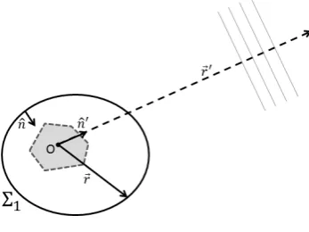
Figure 2.1: Kirchhoff integral formula allows to extrapolate the plane wave far field (~r0→ ∞) from the knowledge of the field near primary or secondary sources (grey area enclosed inside the integration surface Σ1).

A surface Σ = Σ1 ∪Σ2 encloses a region of space V free of sources, which are all contained in the volume inside Σ1 (the grey area bounded by the shaded line). The final calculations are extrapolated in the limit Σ2 → Σ∞,

a spherical surface going at infinity and centered around an arbitrary fixed originOinside Σ1. The asymptotic behavior of the wave field, which becomes that of a plane wave, is analyzed along a direction exiting fromOand defined by the versor ˆn0. The versor ˆn instead, indicates the outward normal to Σ. To derive the Kirchhoff formula one can start from the Green’s function of the scalar Helhmoltz equation in an homogeneos medium:

~

∇2_+k2_g(~r−~r0

) = −δ(~r−~r0)

where k = ω/c (c is the light propagation velocity). The right hand side member represent a point source at ~r0. It is well known [2, 5, 6] that the

fundamental solution with spherical symmetry around~r0 for a homogeneous unbounded medium is:

g(~r−~r0) = e

ikk~r−~r0_k

4πk~r−~r0_k

where the sign in the exponential is coherent with the choice for the time factor e−iωt _{and represents outgoing waves. By considering now the vector}

Helmholtz equation in a source-free region, obtained from the Maxwell’s equations (1.1) expressed in the frequency domain:

~

its fundamental solution (see below) in an unbounded homogeneous medium is the dyadic Green’s function:

¯¯

G(~r−~r0) =

"

¯¯

I+∇~

0_∇~0

k2

#

g(~r−~r0), (2.10) a 3×3 matrix generalization of a vector whose components transform like an R3 second rank tensor and ∇~0∇~0 is the dyadic second order differential operator:

~

∇0∇~0 =X

α X

β

ˆ

αβˆ ∂

2

∂x0

α∂x

0 β

with α, β =x, y, z while ¯¯I is the unit dyadic: ¯¯

I = ˆxxˆ+ ˆyyˆ+ ˆzzˆ=X

α X

β

δαβαˆβ ,ˆ

ˆ

x, ˆy and ˆz being the cartesian orthonormalized basis. Explicitly: ¯¯

G=X

α X

β

Gαβαˆβˆ

where:

Gα,β =gδαβ +

1

k2

∂2_g

∂x0 α∂x0β

. (2.11)

Due to the~r−~r0 dependence of g one has that:

∂2g ∂x0 α∂x 0 β = ∂ 2_g

∂xα∂xβ

.

Bothg and ¯¯G for homogeneous unbounded media are also symmetric in the exchange of arguments~r,~r0. It can then be seen that:

~

∇ ×∇ ×~ G¯¯(~r−~r0)−k2G¯¯(~r−~r0) = ¯¯Iδ(~r−~r0). (2.12) In fact:

~

∇ ×G¯¯ def= X

α X

β X

γ

∂γGαβ(ˆγ×αˆ) ˆβ

2.3. KIRCHHOFF FORMULA AND THE NEAR TO FAR FIELD TRANSFORM21

~

∇ ×∇ ×~ G¯¯ =X

α X

β

(∂α∂βg)ˆαβˆ− X

α

(∇~2_g)ˆααˆ

and the result follows easily when subtracting the k2_G¯¯ _{term and} remem-bering that g is the fundamental solution of the scalar Helmholtz equation. By calculations similar to those in Appendix A, one can also see that an alternative form of (2.10) is:

¯¯

G(~r−~r0) = 1

k2

h

~

∇ ×∇ ×~ Ig¯¯ (~r−~r0)−Iδ¯¯ (~r−~r0)i , (2.13) from which it also follows that:

~

∇ ×G¯¯(~r−~r0) =∇ ×~ Ig¯¯ (~r−~r0). (2.14) Now, if F~ and ¯¯Dare a vector and a dyadic field respectively, it can be shown (see Appendix A) that:

~

∇ ·(F~ ×D¯¯) = (∇ ×~ F~)·D¯¯ −F~ ·(∇ ×~ D¯¯). (2.15) Moreover, after pre-multiplying (2.12) byE~(~r), post-multiplying (2.9) by ¯¯G, subtracting the resultant equation from the first one and integrating with respect to~r over the volume V enclosed by Σ, one has:

~ E(~r0) =

Z

V

dV

h

~

E(~r)·∇ ×~ ∇ ×~ G¯¯(~r−~r0)−∇ ×~ ∇ ×~ E~ ·G¯¯(~r−~r0)i By means of (2.15) it can be shown that the integrand in the above equation equals:

−∇ ·~ hE~(~r)×∇ ×~ G¯¯(~r−~r0) +∇ ×~ E~ ×G¯¯(~r−~r0)i

which after consideration of the (frequency domain) Maxwell’s equationH~ = (∇ ×~ E~)/iωµ and the dyadic identity: A~·(B~ ×D¯¯) = (A~×B~)·D¯¯, allows to write the volume integral as the surface integral:

~

E(~r0) = −

I

Σ

dS

h

ˆ

n×E~(~r)·∇ ×~ G¯¯(~r−~r0) +iωµnˆ×H~(~r)·G¯¯(~r−~r0)i ,

the Dirac delta does not contribute at all. The last steps comprise the limit Σ2 → ∞ with ~r0 fixed, then the limit r0 r. Because all field components

ψ will end up obeying the Sommerfeld radiation condition [5]:

r(∂ψ

∂r −ikψ)→0

for r → ∞, they will look like an outgoing plane wave on Σ∞ (for g this

is directly seen from its explicit expression above), thus the integrands are

o(1/r2_{) in this limit and the integral on Σ}

∞, assumed as a spherical surface

of radiusr=∞ centered atO, vanishes. On the other hand. an asymptotic expression forg when r0 r is:

g ≈ e

ikr0

4πr0 e −i~k0·~r

where~k0 _=knˆ0_{. From this it follows that:}

~

∇g =−i~k0g .

Thus, ifF~ is a fector field, one has:

~

F ·∇ ×~ Ig¯¯ =ig~k0×F~

and

~

F ·∇ ×~ ∇ ×~ Ig¯¯ =ig~k0×~k0×F~ .

By using F~ = ˆn×E~ or F~ = ˆn×H~,one can put the surface integral in the final form:

~

E(~r0) = e

ik~r0

4πi~r0~k 0_×

I

Σ1

dSe−ik·~r

r

µ

h

ˆ

n0 ×nˆ×H~(~r)i−nˆ×E~(~r)

.

(2.16) This is the Kirchhoff integral formula [6], expressing the transverse radiation field far from primary or secondary sources as a function of the angles θ, φ

Chapter 3

Gaussian beams

In the present Chapter E~ and H~ denote frequency domain vector spatial distributions in which the dependence from the (angular) frequency ω is not explicitly indicated. With E~(kx, kz;y), H(~ kx, kz;y) are instead denoted

the spatial Fourier transforms as introduced and described in the previous Chapter 2. The “main” propagation direction is assumed to be the y-axis.

3.1

Paraxial approximation

Often the light wavefield in an optical system propagates along a certain direction y while spreading only slowly in the transverse direction contained in the xz plane. From a quantitative viewpoint this means that, if ~k = (kx, ky, kz) is the wavevector in the field angular spectrum representation,

there is a dominance of ky over kx and kz [18]:

ky = p

k2_−k2

x−kz2 =k

r

1− (k 2

x+k2z)

k2 ≈k− (k2

x+k2z)

2k (3.1)

with k =||~k||. All this means also that in the scalar Helmholtz equation in free space, the solutions are assumed as: ψ(x, y, z) =u(x, y, z)eikyy_{, and the} second derivative of u(x, y, z) along the y-axis is ignored compared to the other second derivatives, in such a way that the paraxial Helmholtz equation becomes [17]:

~

∇2

tu+ 2ik

∂u ∂y = 0

where∇~2

t is thetransverse Laplacian (∂2/∂x2+∂2/∂z2) and k=ω/cwith c

3.2

Gaussian laser beams

To describe a laser beam in its fundamental mode, instead of directly trying a solution of the paraxial Helmholtz equation as in [17], it will be considered an electric field spatial gaussian distribution [18] in the y = 0 plane, the so called focal plane, given by:

~

E(x0,0, z0) =E~oe −x02+z02

w2o ,

whereE~ois a constant vector in the transversexzplane, that will be spatially

transformed aty= 0:

~

E(kx, kz; 0) =

1 4π2

Z +∞ −∞

dx0

Z +∞ −∞

dz0E~oe −x02+z02

w2o e−i(kxx

0_+k

zz0)

=E~o

w2_o

4πe

−(k2x+kz2) w2_o

4

(for the evualuation of the definite integrals see Appendix B). Now, the above espression in used as the angular spectrum in the representation (2.2) of the frequency domain field with (3.1) asky:

~

E(x, y, z) =E~o

w2

o

4πe

iky Z +∞

−∞

dkx Z +∞

−∞

dkze−(k 2

x+k2z)( w2_o

4 +i

y

2k)ei(kxx+kzz), which can be integrated in nearly the same manner as above (see Appendix B) to give the final expression for the paraxial approximation of the vector field in the frequency domain:

~

E(x, y, z) =E~o

eiky

1 +i_kw2y2

o

e

−(x2+z2)

w2_o

1 1+i 2y

kwo2 . (3.2) It should be kept in mind that (3.2) is an approximate solution which does not obey Maxwell’s equations, even if it represents in the y = 0 plane the most realistic achievement of a linearly polarized electromagnetic plane wave. There are also higher order laser modes characterized by different patterns in the focal planeE~ field distribution [18]. The approximation error inherent in (3.1), (3.2) becomes larger the smaller the “beam waist” radius wo is, when

3.3. FOCUSED BEAMS 25

3.3

Focused beams

This section concerns the mathematical description of the electromagnetic field of an optically focalized light beam propagating along a givenaa0 axis. The focalization is made by means of an aplanatic convergent lens having

aa0 as its optical axis and focal length f. The description given here is an adapted and partially modified version from [18,41,42]. Aplanatic (= free of spherical aberration) means that all the in-axis coming rays (from the left, say) converge to the focus F being bended (refracted) in correspondence of a sphere of radius f centered at F behind (to the right) the lens (Gaussian reference sphere). See Fig. 3.1.

𝐹 𝑓

reference sphere

convergent lens ray

𝑎

𝑎′

𝑃 𝑄

Figure 3.1: Scheme of an aplanatic convergent lens with focal lengthfand focus at pointF.P QF is the path of an optical ray.

P Q and QF are conjugate rays. Moreover, if the media of the half-spaces to the left and right of the lens are denoted with the subscript 1 and 2 respectively, then energy conservation gives:

r

1

µ1

kE~1k2dS1 =

r

2

µ2

kE~2k2dS2

where plane wave intensities are assumed for the P Qand QF rays. But: dS2 =

dS1 cos (θ)

of the variable pointQ on the reference sphere is, as a function of the input field amplitude kE~1k:

kE~2k=kE~1k

r_n

1

n2

µ2

µ1

cos (θ). (3.3)

In (3.3) n1,2 =

q

1,2 o

µ1,2

µo are the refractive indices of the media and usually, being µ1,2 ≈ 1, the ratio of the magnetic permeabilities is neglected. Now, assuming the aa0 axis coincides with the y axis of a reference frame with origin in the focal point F, it is possible to apply equation (2.8) to calculate the electromagnetic optically focalized near field in a region of space around

F, using (3.3) as the corresponding far field E~∞. To this end one has to

introduce a further angle φ, besides θ, to measure the azimuthal rotation around theaa0 axis, when the planar integration element dkxdkz is replaced

with a corresponding, more suitable, differential area element on a spherical surface. If theθ angle is measured starting from the negativey semiaxis (to the left ofF, toward the lens) like in Fig. 3.1 — thekx, ky, kz axes coinciding

with thex, y, z ones — these planar and spherical elemental areas are related by:

dkxdkz = cos (θ)k2sin (θ)dθdφ

with k~kk =k and the 1

cos(θ) factor accounting for the projection of the area element on thekxkz plane. But, being ky =−kcos (θ), one has:

1

ky

dkxdkz =−ksin (θ)dθdφ

with which to replace in the double integration of (2.8). Replacing in it also

r with f, one gets:

~

EF(~r;k) =− r

n1

n2

ikf e−ikf

2π

Z θmax 0

Z 2π

0

~

E2(θ, φ;k)eikuˆ·r~cos12 (θ) sin (θ) dθdφ

where:

•θmax is an aperture upper bound due to the finite size of the lens (aperture

stop in a screen and its entrance pupil, which is the image of the entrance stop);

• uˆ is a unit vector pointing from F in the various directions of the solid integration angle;

3.3. FOCUSED BEAMS 27 on that, E~1, of the impinging beam on the lens;

• ~r is the position vector from the focal point F to the point in space in which E~F is calculated.

With reference to Fig. 3.2, there is a change from a cylindrical to a spherical geometry at the reference sphere:

𝐹

𝑎

𝑎′

𝑃 𝑄

𝑥

𝑦 𝑧

𝑛 𝜙

𝑛 𝜌

𝑛 𝜙

𝑛 𝜃

𝜙

Figure 3.2: Reference frame and unit vectors for the electromagnetic field of a focusing aplanatic lens. One sees that the unit vector ˆnφ is unaffected while ˆnρ transforms into ˆnθ.

If the angle φ is measured starting from the x axis in a clockwise sense (i.e., opposite with respect to the right-hand grip rule with the positive y axis as the thumb), using a fixed basis ˆx, ˆy and ˆz one has in general:

ˆ

u= sin (θ) cos (φ)ˆx−cos (θ)ˆy+ sin (θ) sin (φ)ˆz

ˆ

nρ = cos (φ)ˆx+ sin (φ)ˆz

ˆ

nφ =−sin (φ)ˆx+ cos (φ)ˆz

ˆ

nθ = cos (θ) cos (φ)ˆx+ sin (θ)ˆy+ cos (θ) sin (φ)ˆz .

Thus it follows that:

~

E2(θ, φ;k) =tte(θ)

~ E1·nˆφ

ˆ

nφ+ttm(θ)

~ E1·ˆnρ

ˆ

nθ

wherette andttmare the lens transmission amplitudes for the TE (transverse

ideal lens with tte =ttm = 1 and an incident field E~1(θ, φ;k) linearly

polar-ized along thez direction, with a separatedk dependence for the amplitude. As an example, the gaussian monochromatic field distribution of (3.2) with the waist in correspondence of the plane of the lens, which means y = 0 in (3.2):

~

E1(θ, φ;k) = ˆz Eo(k)e

−f2 sin2 (θ)

wo2 = ˆz E_o(k)g(θ, φ).

In fact, x and z in (3.2) are x = fsin (θ) cos (φ) and z = fsin (θ) sin (φ) respectively for small aperture angles. With this choice one has:

~

E2(θ, φ;k) = Eo(k)g(θ, φ) [cos (φ)ˆnφ+ sin (φ)ˆnθ] =Eo(k)g(θ, φ)w~(θ, φ).

By denoting collectively:

~

G(θ, φ) = g(θ, φ)w~(θ, φ) and remembering thatk = ω

c wherecis the phase velocity inside the medium

to the left of the lens (with subscript 2), the above double integral for the focused optical field nearF can be written, assuming for the sake of simplicity

n1 =n2 = 1, as:

~

EF(~r;ω) = −

iωf

2πco

Z θmax 0

Z 2π

0

Eo(ω)G~(θ, φ)e

−i_coω(f−uˆ·~r)

cos12 (θ) sin (θ) dθdφ

where co is the speed of light in vacuum. Multiplying the above

expres-sion by the time phase factor e−iωt_{, integrating over t and remembering the}

correspondence:

iω⇐⇒ −∂

∂t,

it becomes possible to express the optical field in the time domain (by an abuse of notation, the same letters for the time and frequency domain fields are used) as:

~

EF(~r, t) =

f

2πco

Z θmax 0

Z 2π

0 ˙

Eo

t0+ uˆ·~r

co

~

G(θ, φ) cos12 (θ) sin (θ) dθdφ

3.3. FOCUSED BEAMS 29 importance of (3.4) resides in the fact it represent the focused optical field as a superposition of plane waves propagating in the direction opposite to that pointed by ˆu as it scans, with its tip, the given solid angle. In fact, for each

θ and φ fixed, G~, which gives the direction of the E~ field of the superposing waves, is orthogonal to ˆu. Expression (3.4) is similar to those given in [41,42] (see also [43, 44]). The function Eo(t) defines the time profile of the incident

Chapter 4

Planarly multilayered media

4.1

Matrix method for

R

and

T

This section is devoted to the characterization of the reflectanceRand the transmittanceT ofN contiguous layers stacked along theyaxis, each of finite thicknessds(s = 1, . . . , N) and infinite extension in thexzplane, in presence

of a beam of light described by a plane electromagnetic wave impinging on them with a given angle of incidence. The various layers are made of a homogeneous material with a constant absolutecomplex permittivity s:

s=0s+i 00 s

(i is the imaginary unit and the plus sign is coherent with the choice of the sign in the time harmonic phase factor). The complex index of refraction is:

ns =n0s+in 00

s =

r

sµs

oµo

=

r

s

o

.

(s= 1, . . . N) where the last equality holds for non-magnetic (µ≡µo

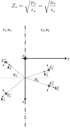
every-where, the vacuum permeability) materials only. Also included are a semi-infinite non-absorptive s = 0 layer with real index of refraction n0, which extends to y =−∞, containing the incident and reflected plane waves, and a semi-infinite s = N + 1 layer which extends to y = +∞, containing the transmitted plane wave. We thus have an overall sequence of N + 2 media identified by the integer s = 0, . . . , N + 1. The xy plane is assumed to be the plane of incidence. Two cases have to be considered: TE-polarization (or s-wave, from “senkrecht” that means perpendicular in German) with the electric field vectorE~ along thez-axis, and TM-polarization (or p-wave, from parallel) with the magnetic field vector H~ along the z-axis.

• Single interface: with a single interface only, the situation is that de-picted in Figs 4.1 and 4.2, where on each side (s = 1 or s = 2) a general superposition of an ingoing and an outgoing plane wave is considered. The field amplitudes on either sides are:

TE: Es,z =

E_s(+)e+iks,yy_+E(−)

s e

−iks,yy_eiks,xx

TM: Hs,z =Zs−1

−E_s(+)e+iks,yy_+E(−)

s e

−iks,yy_eiks,xx

(s= 1,2; the minus sign has been introduced because the vector is entering the plane of the sheet) and Zs is the medium characteristic impedance:

Zs = r

µs

s

=

r

µo

s

𝑥 𝑧

𝑦

𝜀1, 𝜇1 𝜀2, 𝜇2

𝐸1+

𝐸1−

𝐸2+

𝐸2−

𝒌1+

𝒌1−

𝒌2+

𝒌2−

𝜃1

𝜃2

Figure 4.1: TE polarized light on a single interface between two media (E~ points upward from the plane of the sheet, which is the plane of incidence).

where, again, the last equality holds for non-magnetic materials only. By using the curl operator from the Maxwell’s equations in the frequency domain one gets for thetangential components:

TE: Hs,x=

1

iωµs

(∇ ×~ E~s)x =

ks,y

ωµs

E_s(+)e+iks,yy _−E(−)

s e

4.1. MATRIX METHOD FOR R AND T 33

𝑥 𝑧

𝑦

𝜀1, 𝜇1 𝜀2, 𝜇2

𝐻1+

𝐻1−

𝐻2+

𝐻2−

𝒌1+

𝒌1−

𝒌2+

𝒌2−

𝜃1

𝜃2

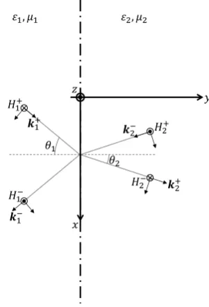
Figure 4.2: TM polarized light on a single interface between two media (H~ points upward from the plane of the sheet, which is the plane of incidence).

TM: Es,x=−

1

iωs

(∇ ×~ H~s)x =

Z−1

s ks,y

ωs

E_s(+)e+iks,yy _+E(−)

s e

−iks,yy_eiks,xx_. (s= 1,2). Here the wave vector lies in the xy plane of incidence:

~ks = ˆxks,x+ ˆyks,y (4.1)

and is in general a complex quantity satisfying:

~ks·~ks=

ω co

ns 2

(4.2) where co is the vacuum light speed. By applying the continuity condition of

the tangential z and x field components for any coordinates at the interface plane y= 0, one gets:

k1,x =k2,x

which is the usual Snell’s law: n1sin(θ1) = n2sin(θ2), if both materials are non dissipative. If thes = 2 medium is absorptive thenk2,x,k2,yand the angle

is non-homogeneous with equal amplitude and equal phase planes having different orientations. For the field amplitudes one instead gets:

TE:

_{1 1}

k1,y

µ1 −

k1,y

µ1 "

E₁(+) E₁(−)

#

=

_{1 1}

k2,y

µ2 −

k2,y

µ2 "

E₂(+) E₂(−)

#

(4.3a)

TM: 1

Z1

k1,y

1 k1,y

1

1 −1

"

E₁(+) E₁(−)

#

= 1

Z2

k2,y

2 k2,y

2

1 −1

"

E₂(+) E₂(−)

#

(4.3b)

where use has been made of matrix notation. Let us callDs(s= 1,2) the 2×2

matrices involved in the above linear relations (4.3) (those in (4.3a) for the TE case, those in (4.3b) for the TM case: this is left understood in all what follows); this allows one to obtain a linear relation among E₁(+), E₁(−), E₂(+)

and E₂(−):

"

E₁(+) E₁(−)

#

= (D1)−1D2

"

E₂(+) E₂(−)

# = a b c d "

E₂(+) E₂(−)

#

from which to calculate the reflection and transmissionamplitudes:

r= E (−) 1

E₁(+) = c a t= E

(+) 2

E₁(+) =

1

a

both calculated imposing the condition: E₂(−) = 0 (note that here, for TM-polarization, the ratio of the electric field amplitudes has been considered and not that of the magnetic ones. This choice is due to the instrumental response, which depends on the electric field). They would give the so called Fresnel coefficients. The single interface example serves as the building block for a sequence of layers.

• Single layer: for N = 1 homogeneous layers (s = 0,1,2), the situation is that depicted in Fig. 4.3, with a near (left) and a far (right) interface of a single slab of thicknessd1 =L.

4.1. MATRIX METHOD FOR R AND T 35

𝑦

0 𝐿

0 1 2

𝐸1 𝑦 = 𝐸1 (+)

𝑒+𝑖𝑘1,𝑦(𝑦−𝐿)

+ 𝐸₁(−)𝑒−𝑖𝑘1,𝑦(𝑦−𝐿)

𝐸0 𝑦 = 𝐸0 (+)

𝑒+𝑖𝑘0,𝑦𝑦

+

𝐸₀(−)𝑒−𝑖𝑘0,𝑦𝑦

𝐸2 𝑦 = 𝐸2 (+)

𝑒+𝑖𝑘2,𝑦(𝑦−𝐿)

+

𝐸₂(−)𝑒−𝑖𝑘2,𝑦(𝑦−𝐿)

Figure 4.3: Single (N= 1) layer with two interfaces. The electric field expressions are for the TE case. For the TM caseZsfactors should appear. The phase factors are the same for both the TE and the TM cases.

"

E₁(+) E₁(−)

#

left

=P1

"

E₁(+) E₁(−)

#

right

=

e−ik1,yL 0 0 e+ik1,yL

"

E₁(+) E₁(−)

#

right

,

one gets after matrix inversion:

"

E₀(+) E₀(−)

#

= (D0)−1

D1P1(D1)

−1

D2

"

E₂(+) E₂(−)

#

.

The use of the propagation matrixP1 amounts to assume the right interfaces as the phase reference planes inside each layer (finite or semi-infinite), with the exception of the last one, in which the left interface plane (obviously) is the phase reference (see again the field expressions in Fig. 4.3).

• Multilayer: from the previous example a pattern emerges, because the above relation can be in a straightforward manner generalized to N layers, by iterating N times the product of the matrices in the curly braces:

"

E₀(+) E₀(−)

#

= (D0)−1∆DN+1

"

E_N(+)₊₁ E_N(−₊₁)

# where: ∆ = N Y k=1

DkPk(Dk) −1

.

The calculation of the overall matrixS for a stack ofN layers plus the initial and final media:

is well suitable for implementation on a computer after specification of: 1) the electric and magnetic (possibly complex) parameters s, µs of the

various N layers at a given angular frequency ω; 2) their thicknessesds;

3) the angle of incidence θ0 of the incoming plane wave in medium s = 0, being assumed to be non-absorptive, which allows, through the chain of equalities (the generalization of the one already seen for theN = 1 case):

ks,x=ks+1,x (s= 1, . . . , N), (4.5)

to calculate the (complex) angleθsin each layer and thus the elements ofDs

and its inverse. In fact from (4.1) and (4.2) one has:

ks,x =

ω co

(n0_s+in00_s) sin(θs)

ks,y =

ω co

(n0_s+in00_s) cos(θs)

and by (4.5), for each s= 1, . . . , N + 1: sin(θs) =

n0₀ n0

s+in00s

sin(θ0) cos(θs) =

q

1−sin2_(θ

s).

From these it follows that:

cos(θs) = s

1− n

02

0(n0s2−n00s2)

(n02

s +n00s2)2

sin2_{(θ0) +i} 2n0sn00sn002 (n02

s +n00s2)2

sin2_(θ0). By putting also:

cos(θs) = qseiγs

qs and γs real with qs>0, one has:

cos2(θs) = q2se

2iγs _=q2

scos(2γs) +iq2ssin(2γs)

and thus by squaring the previous expression for cos(θs) and equating with

the above expression one gets:

q2_scos(2γs) = 1−

n02 0(n

02

s −n

002

s )

(n02

s +n00s2)2

4.1. MATRIX METHOD FOR R AND T 37

q_s2sin(2γs) =

2n0_sn00_sn02 0 (n02

s +n00s2)2

sin2_(θ0)

from which qs and γs can be calculated as functions of θ0, n00, n

0

s and n

00 s.

From these expressions, those for Us≡Re{(n0s+in 00

s) cos(θs)}= c_ωoRe{ks,y}

and Vs ≡Im{ks,y} can be obtained:

Us =n0sqscos(γs)−n00sqssin(γs)

Vs=

ω co

[n0_sqssin(γs) +n00sqscos(γs)].

The reflectance R and transmittance T can be calculated by means of the RMS power flux Pu, along the u axis, from the real part of the complex

Poyinting vector:

Pu =

1 2Re

n

~

E×H~∗·uˆo

where u = x, y, z. If dtot = PN_s=1ds is the total thickness of the multilyer,

which starts at y= 0, and

~k0

s = ˆxks,x−ykˆ s,y,

the fields are (for non-magnetic materials):

TE-polarization)

~

Einc = ˆzE

(+) 0 e

i(k0,xx+k0,yy)

~ Hinc=

1

ωµo

~k0×E~inc

~

Eref l = ˆzrE

(+) 0 e

i(k0,xx−k0,yy)

~

Href l =

1

ωµo

~k0

0×E~ref l

~

Etr = ˆztE

(+) 0 e

i[kN+1,xx+kN+1,y(y−dtot)]

~ Htr =

1

ωµo

~

Einc=−

1

ω0

~k0×H~inc

~

Hinc=−ˆz

1

Z0

E₀(+)ei(k0,xx+k0,yy)

~

Eref l =−

1

ω0

~k0

0×H~ref l

~

Href l = ˆz

1

Z0

rE₀(+)ei(k0,xx−k0,yy)

~ Etr =−

1

ωN+1

~kN+1×H~tr

~

Htr =−ˆz

1

ZN+1

tE₀(+)ei[kN+1,xx+kN+1,y(y−dtot)]_.

Taking account that, by (4.5), k0,x is real (the s = 0 medium is

non-absorptive), that A~ ×(B~ × C~) = B~(A~ · C~)− C~(A~ · B~), and by defining

ξ as the distance (ξ ≥ 0) from the interface at y = dtot, one can get the

following power fluxes at y = 0 (incident and reflected) and at y = dtot

(transmitted) for non-magnetic materials:

Pinc,x =

|E₀(+)|2 2coµo

n0₀sin(θ0)

Pinc,y =

|E₀(+)|2 2coµo

n0₀cos(θ0)

Pref l,x =

|r|2_|E(+) 0 |2 2coµo

n0₀sin(θ0)

Pref l,y =−

|r|2_|E(+) 0 |2 2coµo

n0₀cos(θ0) Ptr,x =

|t|2_|E(+) 0 |2 2coµo

n0₀sin(θ0)e−2Im{kN+1,y}ξ Ptr,y =

|t|2_|E(+) 0 |2 2coµo

co

ωRe{kN+1,y}e

−2Im{kN+1,y}ξ_.

4.2. E~ ANDH~ FIELD DISTRIBUTIONS 39 R=|r|2

T =|t|2 UN+1

n0

0cos(θ0)

e−2VN+1ξ_.

As can be seen, if ξ 6= 0 and the final medium s=N + 1 is dissipative or in the multilayer (s = 1, . . . , N) there is some dissipation and the incidence is not normal, there will be some extra absorption. Ifθ0 = 0 (normal incidence) there is no difference between the TE and TM polarization. In any case the overall matrix (4.4) has to be calculated:

S =





s1,1 s1,2

s2,1 s2,2





and the reflection and trasmission complex amplitudes evaluated:

r= s2,1

s1,1

t= 1

s1,1

.

4.2

E

~

and

H

~

field distributions

Once the reflection and transmission amplitudesr,thave been calculated, the fields inside each layer can recursively be found by applying N times the relations (4.3a) or (4.3b), implying the Ds matrices, starting for example

from the left with:

E₀(+) arbitrary

E₀(−)=rE₀(+)

which correspond to a field in the initial, s = 0, semi-infinite medium given by:

TE: E0,z =E0(+)

e+ik0,yy _+re−ik0,yy_eik0,xx

TM: H0,z =Z0−1E (+) 0

y≤0.

Proceeding recursively one has for the field inside thes-th layer, in terms of the amplitudes of the (s−1)-th medium:

"

Es(+)

Es(−) #

= (DsPs) −1

Ds−1

"

E_s(+)₋₁ E_s(−₋)₁

#

which correspond to a field:

TE: Es,z =

E_s(+)e+iks,y(y−ys)_+E(+)

s e

−iks,y(y−ys)_eiks,xx

TM: Hs,z =Zs−1

−E_s(+)e+iks,y(y−ys)_+E(−)

s e

−iks,y(y−ys)_eiks,xx where:

ys = s X

`=1

d`

with yN =dtot, the total thickness and:

ys−1 ≤y≤ys.

In the final, s=N + 1, semi-infinite medium the field is:

TE: EN+1,z =tE

(+) 0 e

+iks,y(y−dtot)

eikN+1,xx

TM: HN+1,z =−ZN−1+1tE (+)

0 e+iks,y(y

−dtot)_eikN+1,xx with

y≥dtot.

The missing fields can be calculated through (∇ ×~ zEˆ s,z)/iωµs for the TE

4.3. THE INVERSE TRANSMITTANCE PROBLEM 41

4.3

The inverse transmittance problem

As a proposal, the implemented matrix algorithm previously described for evaluating R, T of a multilayer system, could be applied for the inverse problem of determining the refractive index of an unknown material on a given region of the visible spectrum, from measured values of the transmit-tanceT in that range of wavelenghts for a slab fabricated with that material. For sake of definiteness, a trilayer system is considered like the one depicted in Fig. 4.4:

Figure 4.4: Schematic of the measurement....

on which a light beam impinges and from which the experimental transmit-tance is reported. It is a trilayer . Sellmeier [] formula:

n(λ) =

s

1 + H1λ 2

λ2_+K2 1

+ H2λ 2

λ2_+K2 2

+ H3λ 2

λ2_+K2 3

One thus has the analytical transmittance of the trilayer as a scalar-valued function:

T =T (d, H1, K1, H2, K2, H3, K3|λ)

depending nonlinearly from 7 variables and containing also 8 more parame-ters which are the wavelengthλ(explicitly indicated in the expression above), the seven parameters Hsilica

i ,Kisilica (i= 1,2,3) of the Sellmeier formula for

the silica and the thickness of the silica substrate dsilica, which are fixed.

By considering M wavelength values λr (r = 1, . . . , M) on a given range

λmin ≤λ≤λmax, ordered in increasing values and maybe evenly distribuited:

λr =λmin+ (r−1)

λmax−λmin

M −1

one can then consider the vector-valued function (written as a column vector):



 

T (d, H1, K1, H2, K2, H3, K3|λ1) ...

T (d, H1, K1, H2, K2, H3, K3|λM) 

  ,

where every element is theT function calculated at a given λr. By making

M transmittance measuresTmeas

r at the corresponding wavelengths, one can

construct the vector-valued function:

~ F(~p) =



 

f1(~p) ...

fM(~p)   =   

T (d, H1, K1, H2, K2, H3, K3|λ1)− T1meas ...

T (d, H1, K1, H2, K2, H3, K3|λM)− TMmeas 

  ,

where the vector variable~p∈_R7 _{indicates collectively the variables:}

d, H1, K1, H2, K2, H3, K3.

These latter ones will be determined by minimization of the so calledresidual norm, i.e. the scalar valued function:

φ(~p) =

M X

r=1

f_r2(~p)≡ ||F~(~p)||22,

which is a nonlinear least squares problem [1], whose solution is the inverse transmittance problem solution. For ~p∗ to be a minimum of φ(~p) it must necessarily be: ∇~φ(~p∗) = ~0, where ∇~φ(p~ is the gradient of φ(~p). To find

~

p∗ starting from a suitable near point one can use a second order Taylor approximation around a generic point~po:

φ(~po+ ∆~p)≈∇~φ(~po) + ¯¯H(φ(~po))∆~p

where ¯¯H(φ(p~o)) is the Hessian 7×7 matrix of φ(~p): ¯¯

H(φ(~p)) =