Prediction and fusion algorithm for meat moisture content measurement
based on loss-on-drying method
Jing Ling
1*,
Jie Xu
2,
Haijun Lin
3,
Jinyuan Lin
1(1. School of Physics and Electronic-Electrical Engineering, Ningxia University, Yinchuan 750021, China;
2. Department of Food Science and Technology, The Ohio State University, Columbus, OH, 43210, USA;
3. College of Polytechnic, Hunan Normal University, Changsha 410081, China)
Abstract: The loss-on-drying method has been widely used as a standard approach for measuring the moisture content of
high-moisture materials such as solid and semi-solid foods. Loss-on-drying method provides reliable results, whilst usually labor-intensive and time-consuming. This paper presents a novel algorithm for predicting the moisture content of meats based on the loss-on drying method. The proposed approach developed a drying kinetics model of meats based on Fick’s Second Law and designed a prediction algorithm for meat moisture content using the least-squares method. The predicted results were compared with the official method recommended by the Association of Official Analytical Chemists (AOAC). When the moisture content of meat samples (beef and pork) was varied from 69.46% to 74.21%, the relative error of the meat moisture content (MMC) calculated by the proposed algorithm was 0.0017-0.0117, the absolute errors were less than 1%. The testing time was about 40.18%-56.87% less than the standard detection procedure.
Keywords: meat moisture content, loss-on-drying method, Fick’s Second Law, fusion algorithm, measurement, prediction DOI: 10.25165/j.ijabe.20201304.5729
Citation: Ling J, Xu J, Lin H J, Lin J Y. Prediction and fusion algorithm for meat moisture content measurement based on
loss-on-drying method. Int J Agric & Biol Eng, 2020; 13(4): 198–204.
1 Introduction
Food quality issues related to meat products, such as the illegal production of water-injected meat, are attracting a growing public awareness from consumers, industries, and governmental regulators[1]. Due to the temptation of high profits as well as technical difficulties in identifying the water-injected meat, the scandal conditions as mentioned above remain serious[2]. Meat moisture content (MMC) plays an important effect on the quality of meat products, such as color, flavor, and tenderness[3,4]. In recent years, near-infrared spectroscopy[5], ultra-high-performance liquid chromatography-tandem mass spectrometry[6], and multispectral imaging analysis[7] have been developed and applied to identify the water-injected porcine meats. However, these technologists mentioned above are high costs in testing and difficult for commercialization[8]. In this case, an effective and low-cost technique for meat moisture detection is highly needed.
For meat and poultry products, the Loss-on-drying (LOD) method has been approved for official detection purposes according to the international standards recommended by the Association of Official Analytical Chemists (AOAC) 985.14-2005[9] and International Organization for Standardization (ISO) 1442-1997[10]. LOD method permits the simultaneous analyses of large numbers
Received date: 2020-02-14 Accepted date: 2020-04-21
Biographies: Jie Xu, PhD, Postdoc Researcher, research interests: food Science, microbiology and engineering, Email: [email protected]; Haijun Lin, PhD, Professor, research interests: intelligent detection and information fusion system, Email: [email protected]; Jinyuan Lin, MS, Professor, research interests: intelligent detecting and information fusion system, Email: [email protected]
*Corresponding author: Jing Ling, PhD, Associate Professor, research
interests: intelligent detection and information fusion, School of Physics and Electronic-Electrical Engineering, Ningxia University, Yinchuan, Ningxia 750021, China. Tel: +86-15209508892, Email: [email protected].
of samples and does not require equipment calibration[11].
The LOD method provides reliable results, however, complaints about the labor-and time-intensive procedures have been described[12]. Generally, there are two ways to improve the detection efficiency of the traditional LOD method. One is enhancing the heating efficiency during drying, and the other one is using intelligent information processing technology to forecast the measurement results[12,13]. Enhancement of heating efficiency can be achieved via other drying techniques, such as infrared and microwave drying. Compared with the conventional drying methods, infrared drying has a higher drying rate, which is able to reduce the length of drying time with a lower energy cost. The higher drying rate of infrared drying over conventional methods contributes significant time and energy savings[14]. For microwave drying, the major disadvantages lie in the difficulty in temperature control of the final products and the poor temperature uniformity during drying[15]. Moreover, carbonization along the sample corner or edges during microwave drying will result in an inaccuracy of moisture content detection[15].
research work and programming calculation[23].
To simulate an infrared drying process, several empirical or semi-empirical models have been developed to simulate the drying kinetics of various vegetables and fruits[24-26]. However, little information is available regarding the use of the drying model for the detection of meat moisture content based on the LOD method. Therefore, the objectives of this study were: (1) to establish a mathematical model for describing the infrared drying process of meat samples (pork and beef) based on Fick’s Second Law and to verify its adaptability, (2) to develop a prediction and fusion algorithm for meat moisture content detection during infrared drying using the least-squares method (LSM) algorithm, (3) to evaluate the feasibility of the fusion algorithm for meat moisture content detection.
2 Materials and methods
2.1 Preparation of meat samples
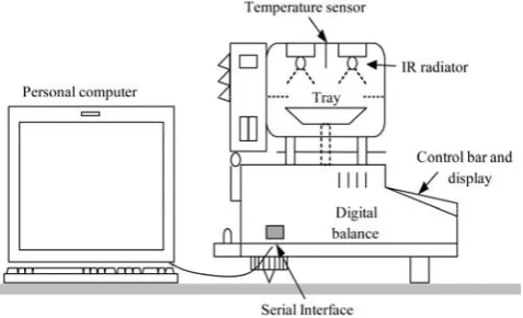
Fresh sirloin (pork and beef) were purchased from the local Walmart supermarket (Changsha, China), with a reference moisture content of the samples varying from 69.46% to 74.21% (wet basis), as determined by the LOD method (AOAC Official Method 2005)[9]. Three replicates were analyzed by the reference method to achieve an analytical variance no more than ±2%. In this study, a moisture analyzer (SARTORIUS, MA100, Germany) was used as the drying apparatus (Figure 1).
Figure 1 Experimental set-up (moisture analyzer equipment: Sartorius, MA100)
2.2 Experimental procedure
For sample treatment, all subcutaneous fat, external fascia, and adhesive tissues were removed from the muscles (pork and beef). The deboned meat chunks were ground by a meat grinder with a blade of 4.0 mm in diameter[27] (Model LM 10K, Koneteollisuus Oy, Finland). As recommended by the AOAC official method 2005, the average weight of the meat samples was 5-6 g[9]. The moisture content of the meat samples (pork and beef) is based on a wet basis (Mwb) in percentage, as expressed by Equation (1)[24,26].
wb 0
100%
t e
m m
M m
−
= ×
(1)
where, mt is the mass (g) of the sample at time t (min); m0and me are the initial and final mass (g) of the sample.
Aluminum drying trays (2 mm in thickness and 90 mm in diameter) were used to hold the meat sample. The tray was pre-dried for a minimum of 1 h at 105°C, cooled in desiccators and weighed[27]. The above procedure was repeated until the difference in weight before and after drying was less than 0.005 g[27]. The moisture content determination was carried out by three independent replicates.
The sample mass was measured every 6 s by the moisture analyzer and uploaded to the computer through the RS-232 interface. The information was then saved in a database and retrieved by the prediction algorithm. All the calculations were processed and programmed by Matlab 2018 (The Mathworks, Inc., Natick, MA, USA).
2.3 Development of the predictive model
Moisture migration in biological products can be driven by a concentration gradient for liquids and by a partial vapor pressure gradient for vapor. The governing equations for moisture transport are Fick’s second law[28,29] as shown in Equations (2) and (3):
0
t
M M
MR
M M
∞ ∞
− =
−
(2)
2 eff
MR D MR
t
∂ = ∇
∂ (3) where, MR is the moisture ratio; t is the drying time (s); Mt is the moisture content at moment t (s); M∞ and M0 is the final and initial moisture content; Deff is the effective moisture diffusivity (m2/s). All the moisture content values are on the wet basis.
Based on the form and characters of samples, the following assumptions are made[30]:
(1) The shrinkage of the product during drying is negligible, and the assumption of one-dimensional heat diffusion is satisfied.
(2) The water diffusion coefficient is constant during drying. (3) External resistance, such as mass transfer resistance, is neglected.
Then, Equations (2) and (3) can be merged into Equation (4),
eff
( )
MR MR
D
t z z
∂ = ∂ ∂
∂ ∂ ∂ (4) where, z is the thickness of the sample (0≤z≤δ) (m). Solutions for Equation (4) with various geometrical and boundary conditions have been compiled by Crank[31]. The solution for an infinite slab is given by:
(
)
(
)
2 2 ff
2 2 2
0 0
8 1 exp 2 1
4 2 +1
t e
n
M M D t
MR n
M M n
∞ ∞ ∞ =
⎡ ⎤
− π
= = ⎢− + ⎥
− π
∑
⎣ δ ⎦ (5)With sufficient drying time, Equation (5) can be simplified by taking the first term of the series solution and assuming that n = 0, which gives[32]
2 eff
2 2
0
8 exp
4
t
M M D t
MR
M M
∞ ∞
⎡ ⎤
− π
= = ⎢− ⎥
− π ⎣ δ ⎦ (6)
Let 2 eff 2
4
D π τ
δ
= , Equation (6) can be rewritten as follows,
0
2 2
8 8
1
t t
t
M e M− e− M
∞
⎛ ⎞
= +⎜ − ⎟
π ⎝ π ⎠
τ τ (7)
Drying is characterized by the simultaneous transfer of heat and mass. A characteristic drying curve of the infrared drying is shown in Figure 2.
derivative of the drying curve is equal to 0. Gradually, the drying rate of the sample slows progressively during the falling rate period (CD), which lasts for a long time, and the second derivative of the drying curve is greater than 0[11,33]. This can be explained by the fact that when the moisture content at the surface decreases and the internal resistance to water transport increases, the evaporated water needs more time to make its way through the dry materials to the evaporation zone[34].
Figure 2 Characteristic drying curve of an infrared drying From Figure 2, it is clear to notice that the moisture content of the meat sample changes dramatically during the heating-up period[29]. In this case, the model developed in this study is not suitable to predict the final moisture content of the sample at this nonstatic stage.
On the other hand, it has been proved that the drying curve during the falling rate period can be described by an exponential model[35]. So, we set the starting point, tc, as the beginning of the prediction algorithm to increase the reliability of our model. This starting point can also be defined as the inflection point. It can be determined by calculating the second derivative of the drying curve. Based on Equation (7), the mathematical drying model of MMC prediction for LOD method can be modified as
( ) ( )
0
2 2
8 8
1
c c
t t t t
t
M e− − M e− − M
∞
⎛ ⎞
= +⎜ − ⎟
π ⎝ π ⎠
τ τ
(8)
2.4 Adaptive recognition for the starting point
The first derivative of the mass and moisture content can be denoted as vm and vM , respectively. The second derivative of mass and moisture content are denoted as am and aM, and regulated by the following equations,
1 1
1
1 0
1 =
i i i m
i i
i i i i
M
i i
dm m m
v
dt t t
dM M M dm
v
dt t t dt m
+ +
+ +
−
⎧ = =
⎪ −
⎪
⎨ −
⎪ = = ⋅
⎪ −
⎩
(9)
2 2
1 1
2 2 2
2 2 2
1 1
2 2 2 2 2
0
Δ ( ) ( )
(Δ) (Δ )
Δ ( ) ( )= 1 Δ
(Δ) (Δ ) (Δ)
i i i i i
m
i
i i i i i i
M
i
d m m m m m m
a
dt t t
d M M M M M M m
a
dt t t m t
− +
− +
⎧ = = = − − −
⎪ ⎪ ⎨
− − −
⎪ = = = ⋅
⎪⎩
(10)
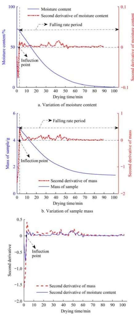
where, mi and mi-1 are the mass of the sample (g) at i and i-1; ti is the drying time in min; Δm and ΔM are the difference in sample mass and moisture content, respectively. Δt is the time interval. From Equations (9) and (10), it can be deduced that the variation trend of the second derivative of the sample mass is the same with that of the second derivative of the sample moisture content. The
inflection point of the drying curve is the same as the inflection point of the sample mass loss.
In this study, pork samples were randomly selected for analysis, with an initial moisture content Mwb=72.76% (wet basis) and initial mass m0=4.991 g. When T=105°C, the infrared drying curve was measured and recorded every 6 s. The derivative of the sample mass and moisture content was then calculated to determine the inflection point, as shown in Figure 3.
a. Variation of moisture content
b. Variation of sample mass
Table 2) was at 3-5 min started from the beginning of the drying process, which was tc in the model. Through the above analysis and calculation, we can determine that tc is the starting point of the falling rate drying period as well as the starting point of our prediction model.
To adjust the experimental data for a better fit, we proposed criteria for the starting point. We set S as a flag to judge the starting point of the estimation algorithm. Upon the above analysis, the starting point of prediction can be determined by judging whether a is positive or negative:
1
1, 0 and 0
0, others.
i i
if a a
S= ⎨⎧⎪ < + >
⎪⎩ (11) where, ai represents the second derivative of sample mass at i. If
S=1, then i+1 is the starting point. However, due to experimental noise, the recorded drying curve is not smooth, so Equation (11) needs to be modified as follows:
1 1
1, 0 and 0 and 0, 1,2,..., ;
0, others.
i i i j
if a a a j K
S= ⎨⎧⎪ < + ≥ + + ≥ =
⎪⎩ (12)
where, K is preset constant, which can be determined from the experiment. If ai+1 meets the requirement of S=1 and the subsequent K points all meet the requirement of a≥0, then i+1 is determined as the starting point of the prediction algorithm.
2.5 Design prediction algorithm based on LSM
According to the multiple regression model, the dependent variable is related to two or more independent variables. The general model is of the form
1 2 1 2
ˆ ( ) ( , , , ; , , , ) ( , )
m k
M t f t t t
f t
β β β
β
= ⋅⋅⋅ ⋅⋅⋅
= JG (13)
where, t1, t2, … tm are independent variables (drying time); β1, β2, … βk are the parameters in the predictive drying model[37].
ˆ ( )
M t is the calculated value of moisture content. Let the observed data points be denoted by
1 1 1 1
( ,t Mc c),(tc+,Mc+), (⋅⋅⋅tc i+,Mc i+), (⋅⋅⋅tc n+ −,Mc n+ −)
(14) where, n is the size of the sliding window (n=20). The problem is to compute those estimates of the parameters which will minimize the error between predictive value and measured value.
( ) ( )
2 2
8 8
[ t tc (1 t tc ) ]
i i c
d M e− − M e− − M
∞
= − + −
π π
τ τ
(15)
The sum of squares of the deviation is
1 1
2 ( ) ( ) 2
2 2
0 0
8 8
{ [ c (1 c ) ]}
n n
t t t t
i i c
i i
Q − d − M e− − M e− − M
∞ = =
= = − + −
π π
∑
∑
τ τ (16)where, M∞is the final moisture content (wet basis) and τ is the coefficient of drying characteristics. According to the principle of the least-squares method[38], Q is the partial derivatives concerning
M∞ and τ, and the derivatives are set to zero. To minimize Q, the two parameters M∞ and τ can be solved by Equation (17)
1 ( ) ( ) 2 2 0 ( ) 2 1 1 ( ) 2 0 0 ( ) ( ) 2 2 8 8
2 [ [ (1 ) ]
8
(1 ) 0
8
2( ) ( ) [
8 8
[ (1 ) ] 0
c c
c
c
c c
n
t t t t
i c
i t t
n n
t t
c c i
i i
t t t t
c
Q M e M e M
M
e
Q
M M t t e M
e M e M
− − − − − ∞ ∞ = − − − − − − ∞ = = − − − − ∞ ⎧ ∂ = ⎧ − + − ⋅ ⎨
⎪∂ ⎩ π π
⎪
⎪ ⎫
− =
⎪ π ⎬⎭
⎪ ⎨∂
⎧
= + ⎨ − ⋅ −
∂ ⎩ π
⎫
+ − ⎬=
π π ⎭
⎩
∑
∑
∑
τ τ τ τ τ τ τ ⎪ ⎪ ⎪ ⎪ ⎪(17)
The goal of our investigation is to find an effective method that will be suitable for embedded systems. Furthermore, the
algorithm can be run by either a small handheld device or an online instrument. To reduce the calculation amount of the algorithm and improve the execution efficiency in the embedded system, we performed the logarithmic operation of Equation (8). By doing this, we can get a linearized fusion expression.
2
8( )
ln( ) ln c ( )
t c
M M
M −M∞ = − ∞ − t t−
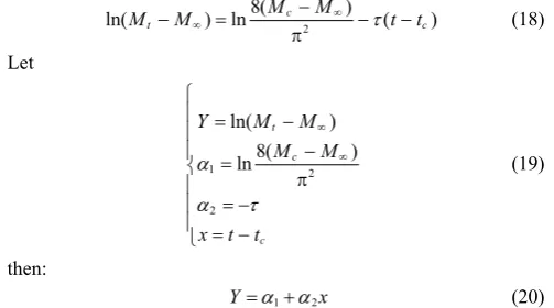
π τ (18) Let 1 2 2 ln( ) 8( ) ln t c c
Y M M
M M
x t t
∞ ∞ ⎧ ⎪ = − ⎪ − ⎪ = ⎨ π ⎪ = − ⎪ ⎪ = − ⎩ α α τ (19) then: 1 2
Y=α α+ x (20) Equation (19) is the information fusion arithmetic expression of meat moisture measurement. These transformations can simplify the data as linear regression for model prediction. After determining α1 and α2, the final dry-basis moisture content M∞ can be calculated.
2.6 Solution of the model parameters
Based on the principle of the least-squares method, the sum of squares of the deviation,ψˆ, can be defined as:
1 1
2 2
1 2
0 0
ˆ n n [ i ( i)]
i i
d y x
ψ − − α α
= =
=
∑
=∑
− +(21)
where, α1 and α2, which minimize ψˆ, can be obtained by the LSM. In the same way, partial derivativesψˆ are taken with respect to α1 and α2, and the following equations are obtained:
1 1
2 1
0 0
1 1 1
2
1 2
0 0 0
n n
i i
i i
n n n
i i i i
i i i
x n y
x x y x
α α α α − − = = − − − = = = ⎧ ⋅ + ⋅ = ⎪⎪ ⎨ ⎪ ⋅ + ⋅ = ⋅ ⎪⎩
∑
∑
∑
∑
∑
(22)
Where α1 and α2 can be obtained by solving the equation:
2 xy
xx
S S
α = ; a1= −y α2x (23)
Let
1 1 1
2
1 1
2
0 0 0
0 0
1 1
0 0
( )
n n n
i i i
n n
i i i
xy i i xx i
i i
n n
i i
i i
x y x
S y x S x
n n y x y x n n − − − − − = = = = = − − = = ⎧ ⎪ ⎪ = − = − ⎪ ⎨ ⎪ ⎪ = = ⎪ ⎩
∑ ∑
∑
∑
∑
∑
∑
(24)
From Equation (19), the relationship between the predicted moisture content M∞ and τ (the coefficient of drying characteristics), α1 and α2 can be obtained:
1 2 2 8 c e
M∞ M
⎧ = −π
⎪ ⎨ ⎪ = − ⎩ α τ α (25)
The iterative algorithm has been applied to calculate the parameters α1 and α2 can be obtained by, and then the prediction of
M∞(the final moisture content) can be obtained. α1(j) and α2(j), the jth approximations of α1 and α2, can be found by inputting sampled data and substituted into Equation (25); that is:
1
2 ( ) ( ) ˆ 8 j j c e
M∞ =M −π
α
The error between Mˆ( )j
∞ (the jth calculated value) and M∞( )j
(the jth measured value) is
1
2 ( )
( ) ˆ( ) ( ) ( )
8
j
j j j j
c e
M∞ M∞ M π M∞
Δ = − = − α − (27)
When Δ(j)=0, the prediction of final moisture content (dry basis) can be obtained. Actually, the above process is equivalent to solving the transcendental equation
1
2
( )
8
c
e
M∞ =M −π −M∞
α
ψ (28)
In order to reduce the influence of the initial value on the convergence of the prediction algorithm, this paper adopts the Newton downhill method[39]. The request to initial value is high in Newton iteration, but the Newton downhill method can extend the range of the initial value.
2.7 Adaptive recognition for the end point
The permitted levels of meat moisture content according to Chinese standard GB 18394-2001[40] are shown in Table 1.
Table 1 Permitted levels of moisture content in livestock and poultry
Category of meat Moisture content/%
Pork ≤77
Beef ≤77
Chicken ≤77
Mutton ≤78
Since these data can be regarded as a priori knowledge of the meat moisture content, we set the first-level threshold value to ɛ1=70% (wet basis). Mˆ∞( )j is the jth predictive value of the sample. If ( )
1
ˆ j
M∞ ≥ε , the value of Mˆ∞( )j would be saved in an array m1[L],
where L is the length of the array. Combining engineering experience and test data, we set L=20.
If the maximal and minimal values meet the following criterion at the same time:
( ) ( )
max 2 min 2
ˆ ˆ ˆ ˆ
|M M j | εand M| M j | ε
∞ ∞
− ≤ − ≤
(29)
We set the parameter ɛ2 as the second level threshold. Through a large number of experiments, we set ɛ2=0.002 as the second-level threshold value to control the accuracy of the
prediction and fusion algorithm. Then Mˆ( )j
∞ is the final
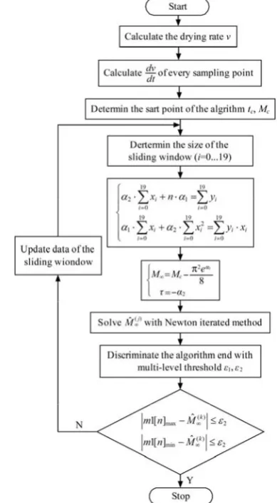
predicted value of the algorithm. The flowchart of the prediction algorithm is shown in Figure 4.
Step 1: The rate of water loss and the first-order derivative during the drying process are calculated;
Step 2: As illustrated in Equation (12), if the next 6 points all meet the requirement of a<0.00001, then i+1 is determined as the starting point of prediction, and then recorded.
Step 3: The sliding window sampling method is applied to the prediction algorithm, and the length of the sliding window array is 20. The predicted value of the final moisture content (wet basis) can be calculated based on the experimental data.
Step 4: The calculated value of the final moisture content (wet basis) is saved. When the online sampling data are updated, they are sent into the data stack and the predicted value of the final moisture content (wet basis) will be updated.
Step 5: ε1 is set as the first-level threshold value to determine whether the predicted value is close to the actual value. At the same time, ε2 is set as the second-level threshold value to control the accuracy of the prediction and fusion algorithm.
Figure 4 Flow chart of online information fusion algorithm for prediction of meat moisture content
3 Results and discussion
3.1 Validation of the predictive model
After the model was built, thirty randomly selected test data from the experiment were used model evaluation. As shown in Table 2, the coefficient of determination (R2) was the primary criterion used to select the most fitted equation for the drying curve, with a reduced chi-square (χ2) and root mean square error (RMSE)[32]. Model evaluation was necessary to estimate the accuracy and robustness of the predictive ability. According to the statistical results shown in Table 2, the R2 of the prediction model is (0.8769-0.9996), χ2 is (1.246×10⁻⁵-1.728×10⁻³), and
RMSE is (0.0073-0.1399), which are regarded as reasonable results.
3.2 Validation of the prediction algorithm
The detection procedure was performed at a drying temperature of 105°C by using the official method. The predicted results were compared with the experimental results. The measurement deviation is presented in Table 3 and Figure 5, and some conclusions can be found as follows:
(1) When the moisture contents of the meat sample (beef and pork) are varied from 69.46% to 74.21%, the relative error of MMC measured by the proposed algorithm is 0.0017-0.0117, the absolute error is less than 1% compared with the official method.
(2) The prediction and fusion algorithm can effectively reduce the detection time while ensuring the detection accuracy. There is about 40.18%-56.87% time reduction in percentage compared with the official method recommend by AOAC.
of samples with an average initial moisture content Mbeef=72.71% for beef or Mpork=70.88% for pork respectively.
Table 2 Curve fitting criteria of mathematical models at different moisture content values
No. Mwb/% m/g R2 χ2 RMSE
70.14 5.605 0.9895 3.725×10⁻⁴ 0.0073
71.34 5.701 0.9712 4.011×10⁻⁴ 0.0451
70.78 4.876 0.9757 3.214×10⁻⁴ 0.0128
71.81 5.112 0.9839 3.132×10⁻⁴ 0.0212
72.32 5.524 0.9909 1.410×10⁻³ 0.0734
69.46 5.012 0.9942 3.041×10⁻⁴ 0.0252
71.15 4.887 0.9966 2.148×10⁻⁴ 0.0135
70.77 5.126 0.9987 1.728×10⁻³ 0.0642
70.87 4.998 0.9863 4.172×10⁻⁴ 0.0155
73.55 5.013 0.9971 4.927×10⁻⁴ 0.0253
70.23 5.045 0.9872 3.527×10⁻⁴ 0.0193
71.44 4.955 0.9995 1.557×10⁻⁴ 0.0395
70.56 5.670 0.9826 2.061×10⁻⁴ 0.0141
72.14 4.668 0.9693 1.449×10⁻⁴ 0.0328
Pork
72.97 4.275 0.9961 1.473×10⁻⁴ 0.0102
70.23 5.533 0.9045 1.483×10⁻⁴ 0.0887
70.98 5.021 0.9985 1.977×10⁻⁴ 0.0105
74.21 5.669 0.9996 2.172×10⁻⁴ 0.0055
73.98 4.778 0.9986 1.358×10⁻⁴ 0.0281
70.33 4.786 0.9994 1.246×10⁻⁵ 0.0091
71.15 4.897 0.8897 1.357×10⁻⁴ 0.0862
72.23 5.126 0.9612 1.751×10⁻⁴ 0.0357
70.88 4.955 0.8899 1.477×10⁻⁴ 0.1399
73.24 4.668 0.9357 1.432×10⁻⁴ 0.0413
71.73 4.711 0.9282 2.666×10⁻⁴ 0.0316
72.56 4.876 0.8769 2.332×10⁻⁴ 0.0889
72.14 5.605 0.9701 2.114×10⁻⁴ 0.0467
72.23 5.002 0.9919 2.623×10⁻⁴ 0.0325
71.92 4.995 0.9956 2.189×10⁻⁴ 0.0177
Beef
71.17 4.997 0.9133 3.477×10⁻⁴ 0.0526
Table 3 Predicted results of moisture content compared with the experimental results
Species Mass /g
Observed value (d.b.)/%
Predicted value (d.b.)/%
Relative error
/%
Measured time /min
Predicted time /min
Time-saving /% 5.605 70.14 70.82 0.0097 97.6 47.6 51.23 5.701 71.34 71.80 0.0064 100.9 51.6 48.86 4.876 70.78 71.45 0.0095 104.6 56.7 45.79 5.112 71.81 71.28 0.0074 102.3 61.2 40.18 5.524 72.32 71.64 0.0094 108.2 60.9 43.72 5.012 69.46 70.04 0.0083 110.2 51.6 53.18 4.887 71.15 70.87 0.0039 109.9 56.3 48.77 5.126 70.77 71.03 0.0036 112.5 55.6 50.58 4.998 70.87 71.01 0.0019 108.3 57.4 46.99 5.013 73.55 72.98 0.0077 111.7 53.5 52.10 5.045 70.23 70.11 0.0017 104.7 62.3 40.49 4.955 71.44 71.05 0.0054 112.8 59.7 47.07 5.670 70.56 69.88 0.0096 106.8 55.3 48.22 4.668 72.14 71.99 0.0021 103.4 44.6 56.87 Pork
4.275 72.97 73.13 0.0022 104.2 60.4 42.03 5.533 70.23 69.95 0.0039 104.3 57.7 44.68 5.021 70.98 70.67 0.0044 107.8 60.2 44.16 5.669 74.21 74.04 0.0023 107.5 57.5 46.51 4.778 73.98 74.22 0.0032 103.4 55.2 46.62 4.786 70.33 70.87 0.0077 99.3 54.2 45.42 4.897 71.15 71.54 0.0056 102.1 49.6 51.42 5.126 72.23 71.99 0.0034 103.7 53.6 48.31 4.955 70.88 71.33 0.0063 102.3 55.7 45.55 4.668 73.24 73.99 0.0102 100.2 58.2 41.92 4.711 71.73 71.12 0.0085 97.2 57.9 40.43 4.876 72.56 72.06 0.0069 99.9 53.6 46.35 5.605 72.14 72.77 0.0087 102.5 57.3 44.09 5.002 72.23 72.67 0.0061 103.3 60.6 41.34 4.995 71.92 71.08 0.0117 99.7 54.4 45.44 Beef
4.997 71.17 71.67 0.0070 101.7 59.5 41.49
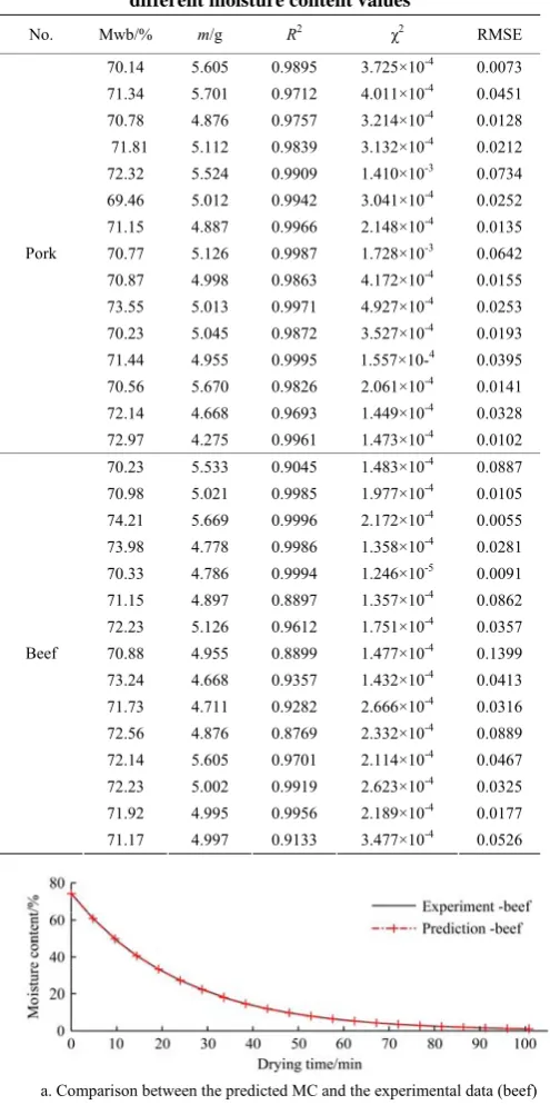
a. Comparison between the predicted MC and the experimental data (beef) b. Comparison between the predicted MC and the experimental data (pork)
c. The verification of predictive error (beef) d. The verification of predictive error (pork) Figure 5 Estimated goodness analysis of the proposed algorithm
The measured curve and prediction curve based on the proposed algorithm of meat samples (beef and pork) are described in Figures 5a and 5b, the verification of predictive error is represented in Figures 5c and 5d. In Figure 5a, the prediction curve is in line with the measured curve for the beef sample,
moisture determination process in pork (shown as Figures 5b and 5d).
4 Conclusions
In this study, a method for rapid determination of moisture content of meat samples based on information fusion technique is proposed. When MMC is varied from 69.46% to 74.21%, the relative error of MMC measured by the proposed algorithm is 0.0017-0.0117, the absolute error is less than 1% compared with AOAC. The time-saving is about 40.18%-56.87% less than the official method. The proposed method could provide a fast and reliable prediction of meat moisture content during the infrared drying process. Also, this algorithm should be useful for developing a new moisture analyzer with a predictive function.
Acknowledgements
This work was supported in part by the National Natural Science Foundation of China (Grant 61663039), and the National Natural Science Foundation of China (Grant 51775185). Equipment and materials for the research were provided by the Natural Science Foundation of Ningxia Hui Autonomous Region (Grant 2020AAC03008).
[References]
[1] Leng Y, Sun Y H, Wang X D, Hou J M, Bai X, Wang M H. A method to detect water-injected pork based on bioelectrical impedance technique. Journal of Food Measurement and Characterization, 2019; 13(2): 1341–1348.
[2] Yang, Y, Wang Z Y, Ding Q, Huang L, Wang C, Zhu D Z. Moisture content prediction of porcine meat by bioelectrical impedance spectroscopy. Mathematical and Computer Modelling, 2013; 58(3): 819–825.
[3] Damez J L, Clerjon S. Meat quality assessment using biophysical methods related to meat structure. Meat Science, 2008; 80(1): 132–149. [4] Huff-Lonergan E, Lonergan S M. Mechanisms of water-holding capacity
of meat: The role of postmortem biochemical and structural changes. Meat Science, 2005; 71(1): 194–204.
[5] Hao D M, Zhou Y N, Wang Y, Zhang S, Yang Y M, Lin L, et al. Recognition of water-injected meat based on visible/near-infrared spectrum and sparse representation. Spectrosc. Spectral Anal, 2015; 35(1): 93–98. [6] Li Z G, Ren N, Ma Y H, Li Y Y, Guo W P. Determination of illegal
drugs for water-retaining in fresh meat by UPLC-MS/MS. Food Sci, 2018; 39(12): 308–312. (in Chinese)
[7] Liu J X, Cao Y, Wang Q, Pan W J, Ma F, Liu C H, et al. Rapid and non-destructive identification of water-injected beef samples using multispectral imaging analysis. Food Chemistry, 2016; 190: 938–943. [8] Liu D, Sun D W, Qu J H, Zeng X A, Pu H B, Ma J. Feasibility of using
hyperspectral imaging to predict moisture content of porcine meat during salting process. Food Chemistry, 2014; 152(1): 197–204.
[9] Analysis of the Association of Analytical Chemists (AOAC). Official methods of analysis Proximate Analysis and Calculations Moisture (M) Meat - item 108. Association of Analytical Communities, Gaithersburg, MD, 17th edition, 2006. Reference data: Method 950.46 (39.1.02); [10] International Organization for Standardization (ISO). Meat and Meat
Products-Determination of moisture content (Routine reference method). Geneva: International Standard ISO, 1997, ISO 1442:1997.
[11] Obi O F, Ezeoha S L, Egwu C O. Evaluation of air oven moisture content determination procedures for pearl millet (Pennisetum glaucum L.). International Journal of Food Properties, 2016; 19(2): 454–466.
[12] Ling J, Teng Z S, Lin H J. Improved method for prediction of milled rice moisture content based on Weibull distribution. Int J Agric & Biol Eng, 2018; 11(3): 159–165.
[13] Ling J, Teng Z S, Lin H J, Wen H. Infrared drying kinetics and moisture diffusivity modeling of pork. Int J Agric & Biol Eng, 2017; 10(3): 302–311. [14] Ruangratanakorn J, Downey G, Allen P, Sun D W. A review of near infrared spectroscopy in muscle food analysis: 2005–2010. Journal of Near Infrared Spectroscopy, 2011, 19(2): 61. doi: 10.1255/jnirs.924. [15] Pu Y Y, Sun D W. Combined hot-air and microwave-vacuum drying for
improving drying uniformity of mango slices based on hyperspectral imaging visualisation of moisture content distribution. Biosystems Engineering, 2017; 156: 108–119.
[16] Nair V V, Dhar H, Kumar S, Thalla K A, Mukherjee S, W. C., Wong J. Artificial neural network based modeling to evaluate methane yield from biogas in a laboratory-scale anaerobic bioreactor. Bioresource Technology, 2016; 217: 90–99.
[17] Liu X Q, Chen X G, Wu W F, Peng G L. A neural network for predicting moisture content of grain drying process using genetic algorithm. Food Control, 2007; 18(8): 928–933.
[18] Gosukonda R, Mahapatra A, Ekefre D, Latimore M. Prediction of thermal properties of sweet sorghum Bagasse as a function of moisture content using artificial neural networks and regression models. Acta Technologica Agriculturae, 2017; 20(2): 29–35.
[19] Singh N J, Pandey R K. Neural network approaches for prediction of drying kinetics during drying of sweet potato. Agricultural Engineering International: CIGR Journal, 2011; 13(1): 1734.
[20] Husna M, Purqon A. Prediction of dried durian moisture content using artificial neural networks. Journal of Physics: Conference Series, 2016; 739(1): 012077. doi: 10.1088/1742-6596/739/1/012077.
[21] Poonnoy P, Tansakul A, Chinnan M. Artificial neural network modeling for temperature and moisture content prediction in tomato slices undergoing microwave-vacuum drying. Journal of Food Science, 2007; 72(1): E042–E047. doi: 10.1111/j.1750-3841.2006.00220.x.
[22] Aghbashlo M, Hosseinpour S, Mujumdar A S. Application of artificial neural networks (ANNs) in drying technology: a comprehensive review. Drying Technology, 2015; 33(12): 1397–1462.
[23] Jafari, S. M., Ganje, M., Dehnad, D., & Ghanbari, V. Mathematical, fuzzy logic and artificial neural network modeling techniques to predict drying kinetics of onion. Journal of Food Processing and Preservation, 2016; 40(2): 329–339.
[24] Sharma G P, Verma R C, Pathare P B. Thin-layer infrared radiation drying of onion slices. Journal of Food Engineering, 2005; 67(3): 361–366. [25] Nowak D, Lewicki P P. Infrared drying of apple slices. Innovative
Food Science & Emerging Technologies, 2004; 5(3): 353–360.
[26] Pekke M A, Pan Z L, Atungulu G G, Smith G, Thompson J F. Drying characteristics and quality of bananas under infrared radiation heating. Int J Agric & Biol Eng, 2013; 6(3): 58–70.
[27] Chinese National standards. Meat and meat products: Determination of moisture content. Beijing: Standard Press of China, 2008, GB 9695.15–2008. (in Chinese)
[28] Doymaz İ. Drying behaviour of green beans. Journal of Food Engineering, 2005; 69(2): 161–165.
[29] Akpinar E, Midilli A, Bicer Y. Single layer drying behaviour of potato slices in a convective cyclone dryer and mathematical modeling. Energy Conversion and Management, 2003; 44(10): 1689–1705.
[30] Sharma G P, Verma R, Pathare P B. Thin-layer infrared radiation drying of onion slices. Journal of Food Engineering, 2005; 67(3): 361–366. [31] Crank J. The Mathematics of Diffusion. Oxford: Oxford University
Press, 1979; 424p.
[32] Wang Z F, Sun J H, Chen F, Liao X J, Hu X S. Mathematical modelling on thin layer microwave drying of apple pomace with and without hot air pre-drying. Journal of Food Engineering, 2007; 80(2): 536–544.
[33] Heldman, Dennis R, Daryl B. Lund, and Cristina Sabliov, editors. Handbook of food engineering. Boca Raton: CRC press, 2018; 1040p. [34] Kocabiyik H, Tezer D. Drying of carrot slices using infrared radiation.
International Journal of Food science & Technology, 200; 44(5): 953–959. [35] Simal S, Femenia A, Garau M C, Rosselló C. Use of exponential, Page's and diffusional models to simulate the drying kinetics of kiwi fruit. Journal of Food Engineering, 2005; 66(3): 323–328.
[36] Zhao D, Ding S X, Karimi H R, Li Y, Wang Y. On robust Kalman filter for two-dimensional uncertain linear discrete time-varying systems: A least squares method. Automatica, 2019; 99: 203–212.
[37] Petkovic M, Neta B, Jovana D. Multipoint methods for solving nonlinear equations. Pittsburgh: Academic Press Inc. 2013; 344p.
[38] Mansard E P D, Funke E R. The measurement of incident and reflected spectra using a least squares method. Coastal Engineering, 1980: 154–172. [39] Luo Y X, Che X Y, Zeng B. Displacement analysis of the 3SPS-3CCS
mechanism based on hyper-chaotic Newton-Downhill method. Key Engineering Materials, 2011; 467-469: 401–406.