www.geosci-model-dev.net/9/3919/2016/ doi:10.5194/gmd-9-3919-2016
© Author(s) 2016. CC Attribution 3.0 License.
A method for retrieving clouds with satellite infrared radiances
using the particle filter
Dongmei Xu1,2, Thomas Auligné2, Gaël Descombes2, and Chris Snyder2
1Key Laboratory of Meteorological Disaster, Ministry of Education (KLME)/Joint International Research Laboratory of Climate and Environment Change (ILCEC)/Collaborative Innovation Center on Forecast and Evaluation of Meteorological Disasters (CIC-FEMD), Nanjing University of Information Science & Technology, Nanjing 210044, China
2National Center for Atmospheric Research, Boulder, Colorado 80301, USA
Correspondence to:Dongmei Xu ([email protected])
Received: 11 June 2016 – Published in Geosci. Model Dev. Discuss.: 4 July 2016
Revised: 13 September 2016 – Accepted: 10 October 2016 – Published: 2 November 2016
Abstract.Ensemble-based techniques have been widely uti-lized in estimating uncertainties in various problems of inter-est in geophysical applications. A new cloud retrieval method is proposed based on the particle filter (PF) by using en-sembles of cloud information in the framework of Grid-point Statistical Interpolation (GSI) system. The PF cloud retrieval method is compared with the Multivariate Mini-mum Residual (MMR) method that was previously estab-lished and verified. Cloud retrieval experiments involving a variety of cloudy types are conducted with the PF and MMR methods with measurements of infrared radiances on multi-sensors onboard both geostationary and polar satellites, re-spectively. It is found that the retrieved cloud masks with both methods are consistent with other independent cloud products. MMR is prone to producing ambiguous small-fraction clouds, while PF detects clearer cloud signals, yield-ing closer heights of cloud top and cloud base to other ref-erences. More collections of small-fraction particles are able to effectively estimate the semi-transparent high clouds. It is found that radiances with high spectral resolutions con-tribute to quantitative cloud top and cloud base retrievals. In addition, a different way of resolving the filtering problem over each model grid is tested to better aggregate the weights with all available sensors considered, which is proven to be less constrained by the ordering of sensors. Compared to the MMR method, the PF method is overall more computation-ally efficient, and the cost of the model grid-based PF method scales more directly with the number of computing nodes.
1 Introduction
instru-ments. However, MMR has limitations in several aspects due to its use of minimization for solution: (1) part of the control variables accounting for the cloud fraction for some certain levels are under-observed since the channels are not sensitive to the existence of clouds for those heights; (2) when clouds at different heights show opacities with the same spectral sig-nal, MMR could lose the ability to distinguish solutions in-volving clouds at those levels; (3) the computational cost for the minimization procedure in MMR is rather considerable.
Ensemble-based techniques, which usually reside in short-term ensemble forecasting (Berrocal et al., 2007; Shen and Min, 2015), assembling existing model outputs (e.g., cloud retrievals) from varying algorithms (Zhao et al., 2012), or ensemble Kalman filter (EnKF) in diversified forms (Snyder and Zhang, 2003), have been widely developed in order to estimate the uncertainties of various problems in geophysical applications. To better account for the non-linearity between the observed radiance and the retrieval parameter, a novel prototype for detecting clouds and retrieving their vertical extension inspired by the particle filter (Snyder and Zhang, 2003; van Leeuwen, 2010; Shen and Tang, 2015) technique and Bayesian theory (Karlsson et al., 2015) is proposed in this study. As a competitive alternative for MMR, the PF trieval method has same critical inputs required and cloud re-trieval products as in MMR. A brief description of MMR and the new PF cloud retrieval algorithm are provided in the fol-lowing section. Section 3 describes the background model, the data assimilation system, the radiative transfer models (RTMs) and the radiance observations applied in this study. Model configurations are also illustrated in Sect. 3. In Sect. 4, the single test within one FOV is conducted before the per-formance of PF method is assessed by comparing its cloud retrievals with those from MMR and other operational cloud products. Section 4 also discusses the computational perfor-mance for the two methods. The conclusion and anticipated future work are outlined in Sect. 5.
2 Methodology
Essentially, the PF cloud retrieval scheme retrieves clouds with the same critical inputs requested (i.e., clear-sky radi-ance from the radiative transfer model and the observed ra-diance) and the same cloud retrievals as outputs (i.e., three-dimensional cloud fractions, which is defined as the fraction of top of cloud as seen from a sensor) with the MMR method. Both cloud retrieval schemes consist of finding cloud frac-tions that allow for best fit between the cloudy radiance from model and the observation. We use c1, c2, . . ., cK to denote the array of vertical effective cloud fractions for K model levels (c1for the surface andcKfor the model top) andc0as the fraction of clear sky with 0≤ck≤1, ∀k∈ [0, K]. The constraint for the cloud fraction is as follows:
K X
k=0
ck=1 (1)
In this study, a cloud on one model level with a given frac-tionckis assumed to block the radiation from its lower model levels. The radiation originating from its lower levels is as-sumed to contribute to the top of atmosphere radiance ob-served by the satellites only with the residual fractions.
The MMR method is an approach to retrieve cloud frac-tions using the minimization technique. The residual of the modeled radiance and the observation is normalized by the observed radiance, which results in the following cost func-tion, usingck,∀k∈ [0, K]as the control variables:
J (c0, c1, c2, . . ., cK)=1
2 X
v
Rcloud
ν −Rνobs Robs
ν
2
, (2)
whereRcloudv is the modeled cloudy radiance, andRobsv the observed radiance at frequencyv. This vertical cloud frac-tionc1, c2, . . ., cK andc0 are control variables for the cost function, where the simulatedRcloudv is defined as
Rvcloud(c0, c1, c2, . . ., cK)=c0R0v+
K X
k=1
ckRvk. (3)
HereRvk is the radiance calculated assuming an overcast black cloud at the model level k andR0v the radiance cal-culated in the clear sky. BothRkv andRv0are calculated us-ing a forward radiative transfer model with model profiles of temperature and moisture as inputs. Details of the schematic of the MMR method can be referred to in Descombes et al. (2014) and Xu et al. (2015).
Particle filter (PF) approach is one of the non-linear filters for data assimilation procedures to best estimate the initial state of a system or its parametersxt, which describes the
time evolution of the full probability density functionp(xt)
conditioned by the dynamics and the observations. Similar to the study in Mechri et al. (2014), the bibliography on PF focuses on estimating the parameters, which are cloud frac-tionsck in Eq. (3), in this study. While MMR retrieves the cloud fractions on each model vertical level by minimizing a cost function, PF calculates posterior weights for each en-semble member based on the observation likelihood given that member. In its simplest form, PF works by initializing a collection of cloud profiles as particles and then estimat-ing the cloud distributions by averagestimat-ing those particles with their corresponding weights. Each particle’s weight is com-puted with the difference between the modeled cloudy radi-ance from the particle and the observed radiradi-ance.
members; i.e., one cloud profile as one of particles is corre-sponding to an ensemble member.
Two approaches for generating particles are initially de-signed; the first one is to generate the perturbed sam-ples Cbi(∀i∈ [1, n]) from the cloud profile in the back-ground denoted asCb=(c0b, c1b, . . ., cKb)by inflating (deflat-ing) the clouds with small magnitudes (Cb=α×Cb, α=50, 55,. . . , 150 %) and moving upward (downward) with δz= +5,+4. . .,−1, . . .−5 as the vertical magnitude, wherenis the sample size. The perturbed cloud fractions are designated to replenish the ensemble by introducing the prior informa-tion of the cloud distribuinforma-tions from the background and to increase the ensemble spread.
Besides those perturbed particles, to represent the exis-tence of a one-layer cloud on each model level with an even chance, another diversity set of profilesCib(∀i∈ [1, K+1])
are also initialized, among which Cbi stands for the profile with 100 % cloud fraction on the model leveli(ci =100 %) and 0 % cloud on the rest levels. In particular, Cb0 defines 100 % clear (c0=1). It is also interesting to discretize the initial particles by setting the one-layer cloud with the value ofci from 100 to 0 % (e.g., 100, 90, 80, . . . , 0 % with 10 % as the interval) and further from 100 to 0 % (e.g., 100, 99, 98, 97, . . . , 0 % with 1 % as the interval). In this cases,
c0=1−ci. For each particleCbi, its simulated cloudy radi-anceRcloudv,i from the model background can be obtained with Eq. (3).
A cost functionJois defined for each particle to measure
how the particle fit the observation as
Jo=
Robsν −Rν,icloud σ
!2
. (4)
σ is the specified observation error, which can be referred to in the first paragraph in Sect. 4.1. The weightwifor each par-ticleCbi is thus calculated by comparing the simulatedRv,icloud
and the observation Rvobsusing the exponential function by accumulating theJofor multiple frequency as
wi=e −P
v
Robsν −Rcloudν,i σ
!2
, (5)
∀i∈ [1, n]. Herenis the particle size andσ is the specified observation error, which can be referred to in the first para-graph in Sect. 4.1. The final analyzedCais obtained by aver-aging the background particlesCbi with their corresponding weight, as
Ca=
p X
i=1
wiCbi. (6)
In Eq. (6), the constraint referred to in Eq. (1) is not re-spected. Thus, after the analysis step for the particle filter,
the final averaged cloud fractionsckaare normalized by
cak= c
k K P
k=0
ck
, (7)
where∀k∈ [0, K].
3 Data and model configurations 3.1 Data
The Advanced Infrared Sounder (AIRS), the Infrared Atmo-spheric Sounding Interferometer (IASI) and the Cross-track Infrared Sounder (CrIS) are among the most advanced hy-perspectral infrared sounders and thus are applied for re-trieving clouds with hundreds of channels (Blumstein et al., 2004; Aumann et al., 2003; Xu et al., 2013; Bao et al., 2015; Smith et al., 2015). The Radiance measurements from Mod-erate Resolution Imaging Spectroradiometer (MODIS) on-board the Earth Observing System (EOS) Terra or Aqua satellites are also well suited to extracting valuable cloud information from the 36 spectral broadband frequencies in the visible, near-infrared and infrared regions at high spatial resolution (1–5 km) (Ackerman et al., 1998). Apart from the IR radiances from polar satellites, the Geostationary Opera-tional Environmental Satellite (GOES) Imager (Menzel and Purdom, 1994) provides a continuous stream of data over the observing domain. In this study, 13 (east) and GOES-15 (west) are also utilized to obtain cloud fractions over the continental United States (CONUS) domain. The GOES Im-ager used in this study is a five-channel (one visible, four infrared) imaging radiometer designed to sense radiant and solar reflected energy. The instrument parameters for the sen-sors and the setups for channel selections can be found in Xu et al. (2015).
3.2 WRF, GSI and the radiative transfer model
3.3 Model configurations
The WRF is configured with 415×325 horizontal grids at 15 km grid spacing, and 40 vertical levels up to 50 hPa within the single CONUS domain. The MMR and PF cloud de-tection schemes search the cloud top using approximately 150 hPa as the highest extent for most cloudy cases. Other clouds higher than 150 hPa, e.g., an anvil cloud in a mature thunderstorm around tropopause at low latitude region, will also be explored in future studies. Channels in the long-wave region are utilized following the channel selection scheme in (Xu et al., 2015). Since the final retrieval clouds are on model grids, the retrieved cloud fractions within one FOV are essen-tially extrapolated to its four neighboring model grid points. Generally, for each FOV, the retrieved cloud fractions are ex-trapolated to its four neighboring model grid points. For polar satellite pixels, the representative cloud fractions are extrap-olated with an adaptive radius with respect to their scan po-sitions. The cloud detecting procedure for retrieving clouds is conducted for each FOV from each individual sensor in-dependently and sequentially. Since the clouds are retrieved FOV by FOV and the clouds on grids are referred to imme-diately after one FOV is completed, there is no obvious ac-curacy loss of radiance observations using this conservative method.
4 Experiments and results
The PF experiments apply two groups of particles as men-tioned in Sect. 2, among which the group 2 particles contains solely 100 % one-layer clouds. To reveal how the setup of the initial particles impacts the results, apart from the MMR and PF experiments, we included another advanced experiment, denoted as Advanced PF (APF). APF requires more sampled particles including ranges of cloud fractions spanning from 0 to 100 % at intervals of 10 %. An additional experiment “APFg2”, similar to APF but excluding the perturbed parti-cles from the background in group 1 introduced in Sect. 2, was conducted to evaluate the added values from the group 1 particles. In this section, cloud retrieval experiments for several cases containing clouds of a variety of types are con-ducted for comparison reason. The GOES imager retrieved products from National Aeronautics and Space Administra-tion (NASA; Langley cloud and radiaAdministra-tion products) are ap-plied as a reference to validate the cloud retrieving methods for the CONUS domain with a large and uniform coverage of cloud mask. In addition, the retrieved cloud products were also compared to available CloudSat (Stephens et al., 2002) and MODIS level 2 cloud products (Platnick et al., 2003) archived by the CloudSat Data Processing Center in Col-orado State and NASA, respectively.
V
ertical model level
Pressure (hPa)
Clear sky
Figure 1.Ratio of the overcast radiances vs. the observed radiance starting from the level 1. The ratio of the clear-sky radiance normal-ized by the observed radiance corresponds to level 0 (see text for explanation) for the GOES-Imager for channel 5. The approximate pressures corresponding to the model levels are also denoted.
4.1 Single test at one field of view
The PF cloud retrieving algorithm retrieves the cloud distri-butions by averaging those initial particles with their weights. Before the real case experiments are carried out over the whole domain, we conduct a single cloud retrieving test at one FOV to understand what differences can be explained by the differences in the basic initial particles. In Eq. (5), the observation errorσ can be set proportional to the observa-tion equalingRvobs
r , whereris the prescribed ratio. Thus, the
cloud signals on each levelkare virtually determined by the extent of how close the Rkv
Robs
v
(and Rv0
Robs
v
for the clear part) gets to 1. An example of the ratio of the overcast radiance and the observed radiance Rkv
Robs
v
for each model level is given in Fig. 1 of the GOES-Imager for the channel 5 (∼13.00 µm). The clear-sky radiance normalized by the observed radiance
R0
v
Robs
v
is also shown at the level 0 (Fig. 1). It is expected that the overcast radiance from the RTM decreases with the rising of the altitude. The cloud signal is strongest around level 5, whereRvkfitsRvobsmost closely. The cloud retrievals depend not only on the basic input profiles (i.e., the overcast radi-ance on each level from RTM normalized by the observed radiance and the clear-sky radiance from RTM normalized by the observed radiance) and but also on the algorithm ap-plied for resolving the problem (e.g., MMR and PF in this study).
(a) (b)
Model level Model level
Cloud fraction Cloud fraction
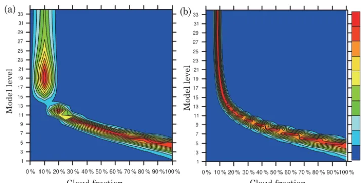
Figure 2.The weights for different particles with specified cloud fractions on thexaxis at one chosen model level shown on theyaxis from
0 to 100 %(a)at the interval of 10 % and(b)at the interval of 1 %.
ck (on thexaxis) on specified model levelsk(on theyaxis) from 10 to 100 % every 10 %. With a fraction ck of one-layer cloud at a given level kand a fraction of c0=1−ck
of clear sky, the simulated cloudy radiance can be denoted as
Rvcloud=ckRkv+(1−ck)R0v. Hence the theoretical one-layer cloud fraction is solved as ck=R
0
v−Robsv
R0
v−Rkv
by fitting Rvcloud
to Rv0. As expected, for one-layer cloud with full fraction,
c5equals 100 %. In light of the concept thatRvk> Rkv+1, no cloud can be present below level 5 since this would implies a
Rvcloudlarger than the observation (or aci larger than 100 %). It seems that clouds can be described by different possible states as particles with both large fractions and small frac-tions. Low clouds are easily estimated by one-layer cloud profile with large fractions (larger than 10 %). The particles with small-fraction high clouds gain some weights to retrieve high clouds. The particle with the one-layer cloud on level 13 seems to gain least weight compared to the others levels. The weights for the particles with cloud fractions from 0 to 100 % at the interval of 1 % are also presented in Fig. 2b. By includ-ing more small-fraction one-layer clouds, the clouds around level 13 can be reproduced by the group of refined particles with 1 % as the interval for approximately 10 % cloud frac-tions. However, changing the level of the cloud for the fixed fraction (10 %) does not seem to change the outgoing radi-ance much, probably due to the channel’s low weight func-tion peak (∼750 hPa).
The normalized Jo in Eq. (6) for different levels with a
specific cloud fraction from 0 to 100 % every 10 % are shown in the bottom panel of Fig. 3, with 10 and 1 % as the intervals in Fig. 3c and d, respectively. Here,Jocan be further derived
as
Jo=r2
1−c0 R
0
v Robs
ν
−ck R k v Robs
ν 2
, (8)
with σ =Rvobs
r and R
cloud
v (c0, c1, c2, . . ., cK)=c0Rv0+ K
P
k=1
ckRvk.
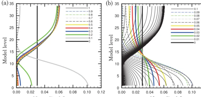
From Fig. 3a, it is found thatJois smallest around level
5 with 100 % cloud fraction (denoted as 1 in legend) for the thin black line, with respect to the fact that the overcast ra-diance fits the observed rara-diance most closely for level 5 ap-proximately. The gray line with 10 % cloud fraction (0.1 in the legend) corresponds to the existence of a weight peak on level 19 in Fig. 2a. In addition, the gap between the gray line with 0.1 and the other lines from 0.2 to 1 explains why there’s less continuity around level 13. Figure 3b shows a similar pattern to Fig. 3a, except with densely distributedJovalues around the level 13 from 0.1 to 1 in the legend. Those con-tiguous black lines in Fig. 3b are associated with the set of particles with cloud fractions from 10 to 100 % at the interval of 1 %.
4.2 Cloud profiles
Normalized Jo Normalized Jo
Model level Model level
(a) (b)
Figure 3.The normalizedJo(a)at the interval of 10 % and(b)at the interval of 1 %. In(b), the normalizedJofrom 0.1 to 1 are all denoted
as black lines.
of low clouds; by adding a set of particles with small-fraction clouds in APF, higher clouds can be reproduced, which is consistent with the implications from Figs. 2b and 3b. APF detects clear strong cloud signals and removes the cloud frac-tions on near-surface levels around 36◦N successfully. Since the existence of ground-layer radar reflectivity is likely cor-responding to the strong reflection from the underlying sur-face of the Earth, the height of cloud bases of MMR and PF are not compared in this sub-section. The experiments with a larger size of particles including 0 to 20 % (at the interval of 1 %) plus 30 to 100 % (at the interval of 10 %) or of 0 to 100 % (at the interval of 1 %) one-layer cloud profiles (intro-duced in Sect. 2) yield similar results from APF but are much more costly (not shown).
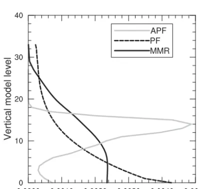
The vertical profiles of the averaged cloud fractions from MMR, PF and APF are plotted in Fig. 5 at 11:00 UTC, 3 June 2012, with AIRS. Both MMR and PF experiments yield ambiguous cloud distributions, whereas APF retrieves much stronger cloud signals constrained between level 2 to level 20 (approximately from 950 to 400 hPa). More clouds around level 10 are retrieved (approximately 750 hPa) in MMR, while PF is prone to retrieving clouds near surface levels. Note that MMR retrieves much higher cloud tops and lower cloud bases compared to APF. The cloud base from PF is the lowest; the cloud top from MMR and PF is compara-ble. Only the APF-related methods will be further discussed in later sections, due to the absence of high clouds using PF.
4.3 Cloud mask
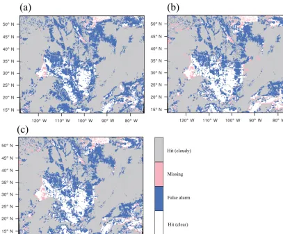
Comparison experiments on real cases are further performed for over longer time period from 00:00 UTC, 12 Decem-ber 2013, to 07:00 UTC, 12 DecemDecem-ber 2013. The cloud mask is marked as cloudy when there is a recognizable existence of cloud on any level from MMR or PF retrievals. Both the NASA GOES Imager products and the MMR-retrieved fields
are interpolated to the same 0.1◦×0.1◦ latitude–longitude grid with 0 for clear and 1 for cloudy before the compar-isons for verification. Figure 6 shows thehits,false_alarms andmisseslocations with the use of GOES-Imager, MODIS, CrIS, AIRS and IASI radiances in the retrieval algorithms at 07:00 UTC, 12 December 2013. Note that cloud mask re-trievals from both the MMR and APF hit the clear and cloudy events well in Fig. 6a and b. In most areas, the MMR exper-iment overestimated the cloud mask with more false alarm events compared to the APF experiment, since the MMR so-lution is an “overly smoothed” estimation of the true vertical profile. It seems that the accuracy of cloud detection is lower for areas with high altitude than under tropical conditions, indicating that the smaller lapse rate in the atmosphere will lead radiance less sensitivity to clouds over polar areas. Fig-ure 6c shows the cloud mask results from the APFg2 experi-ment without the perturbed particles in group 1 introduced in Sect. 2. There is no large discrepancy between Fig. 6b and c, suggesting that the particles in group 2, which fully span the possibility of the cloud distributions, are more determinant in retrieving the cloud mask.
4.4 Cloud top and base pressure
(b)
(c)
(d)
(a)
Figure 4. (a)The radar reflectivity (units: dBZ) cross sections from CloudSat,(b)the MMR retrieved cloud fraction (units: %) cross sections,
(c)the PF retrieved cloud fractions and(d)the APF retrieved cloud fractions valid at 11:00 UTC, 3 June 2012.
Figure 5.The mean cloud fraction on all model levels for the ex-periments MMR, PF and APF with AIRS observations valid at 11:00 UTC, 3 June 2012.
overestimation of the CBPs is even more obvious from MMR in most regions in Fig. 7d.
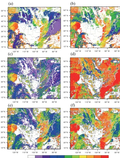
The CTPs from NASA GOES cloud products for more hours (03:00, 05:00, 07:00 UTC) together with the in-dependent CTP retrievals from MODIS level 2 products
(http://modis-atmos.gsfc.nasa.gov/MOD06_L2/) are plotted in Fig. 8. Different sub-periods of the MODIS cloud retrieval products (e.g., Fig. 8b valid at 03:20 UTC, Fig. 8c at 03:25, and Fig. 8d at 03:30 UTC) are chosen to approach the valid times in Fig. 8a, e and h. The CTPs from both cloud prod-ucts agree well for both high and low clouds, confirming that NASA GOES cloud products are overall reliable for verify-ing the cloud retrievals and MODIS level 2 products can also be applied for validations.
Hit (clear) False alarm Missing Hit (cloudy)
(a)
(b)
(c)
Figure 6.The false alarms, misses and hits for clear and cloudy event locations with(a)the MMR method,(b)the APF method and(c)the APF method but without the group 1 particles (see text for detailed explanations) valid at 07:00 UTC, 15 December 2013.
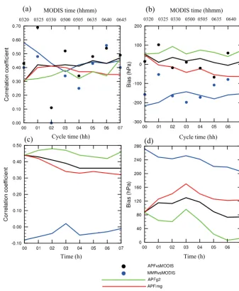
the CTPs from MMR are underestimated (putting the clouds too high) consistently against both retrievals with GOES and MODIS radiances. Figure 9c shows that the correlations are weaker for MMR compared to others all the time. In Fig. 9d, the positive CBP biases from MMR are remarkable, whereas the CBP biases from APF are largely reduced. Generally, AP-Fimg degrades the CTP and CBP results consistently, sug-gesting that radiances with high spectral resolutions are able to improve the vertical descriptions of cloud profiles. It is found that the clouds retrieved with APFg2 are shrunken in terms of cloud depth with notably lower cloud top and higher cloud base compared to APF, when excluding the perturbed particles in the first group.
4.5 Computational issues
Figure 10a represents the elapsed times for the MMR and APF experiments and the counts of radiance observations in use are shown in Fig. 10b from 00:00 to 07:00 UTC, 12 De-cember 2013. The profile of computing time in MMR is quite different from that in PF. The cost of MMR is dominated by the heavy minimization procedure, whereas APF is more
as-sociated with the processes of initializing particles and calcu-lating weights for all the particles. The computing times were measured from cloud retrieving runs with 64 MPI (Message Passing Interface) tasks on a single computing node in an IBM iDataPlex Cluster. The measured wall clock comput-ing times show that generally MMR is computationally more expensive for most of the time than APF. It seems the wall clock times for MMR are generally proportional to the data amount used. While for the APF experiment, the wall clock time is mostly determined by the particles size and partly af-fected by the channel number, such as for 2013121202 and 2013121206, when the total counts of the hyperspectral sen-sors (IASI, CrIS and AIRS) are large. The PF experiments using particles of the one-layer cloud with 100 % cloud frac-tions usually take less than 5 min for the same periods (not shown).
re-(a)
(b)
(c)
(d)
(e)
(f)
(hPa)
Figure 7.The cloud top pressure (left panels) from(a)the NASA GOES retrieval,(c)the MMR method and(e)the APF method, and the
cloud bottom pressure (right panels) from(b)the NASA GOES retrieval,(d)the MMR method and(f)the APF method valid at 07:00 UTC,
15 December 2013.
trieved cloud fractions are extrapolated to its neighboring model grid points afterwards. We order the sensors in the cloud retrieving procedure as GOES-Imager, MODIS, CrIS, AIRS and IASI, aiming to optimize the vertical clouds
(a)
(e)
(h)
(b)
(f)
(i)
(c)
(d)
(g)
(j)
(k)
0320
0325
0330
0500
0505
0635
0640
0645
(hPa)
Figure 8.The cloud top pressure for(a)03:00 UTC from the GOES NASA retrieval;(b)03:20 UTC,(c)03:25 UTC and(d)03:30 UTC from
MODIS level 2 products;(e)05:00 UTC from the GOES NASA retrieval;(f)05:00 UTC,(g)05:05 UTC;(h)07:00 UTC from the GOES
NASA retrieval;(i)06:35 UTC,(j)06:40 UTC and(k)06:45 UTC from MODIS level 2 products.
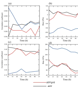
other hand, it means the information from other prior sensors will be more or less discarded. In this section, a different way of resolving the filtering problem is preliminarily tested, in which the weights for each particle are aggregated over all available sensors by calling the forward radiative transfer model on neighboring model grids.
0320 0325 0330 0500 0505 0635 0640 0645 0320 0325 0330 0500 0505 0635 0640 0645
(a) (b)
(c) (d)
MODIS time (hhmm) MODIS time (hhmm)
Cycle time (hh) Cycle time (hh)
Time (h) Time (h)
Figure 9. (a)Correlation coefficient,(b)bias for the cloud top pressure,(c)correlation coefficient and(d)bias for the cloud bottom pressure vs. the NASA GOES retrievals from 06:00 UTC, 15 December 2013, to 07:00 UTC, 15 December 2013. Black and blue dots denote results vs. the MODIS level 2 cloud top pressure retrieval valid at 03:20, 03:25, 03:30, 05:00, 05:05, 06:35, 06:40 and 06:45 UTC. The valid times
for the MODIS level 2 data are shown on the top of thexaxis.
available for most of the time. It is worth pointing out that the ordering of different sensors has nearly no effect on the final cloud retrievals, when the weights of the particles are calculated in model space (not shown). The final cloud re-trieval is no longer overwritten by the rere-trieval from the last sensor but is a total solution with all the sensors fairly con-sidered, instead. The computational cost of retrieving clouds in model space is comparable or slightly heavier than that in observation space. The computational cost of the grid-based scheme scales with the number of the computing nodes more directly, compared to that of the FOV-based scheme.
5 Discussion and conclusion
(a) (b)
Time (h) Time (h)
Figure 10. (a)The elapsed time and(b)the data count from 00:00 to 07:00 UTC, 15 December 2013.
(a)
(b)
(c)
(d)
Time (h) Time (h)
Time (h) Time (h)
cloud top pressures (put the clouds top too high) and over-estimates the cloud bottom pressures (put the clouds top too low) as well. APF improves both the retrievals of cloud tops and cloud bases remarkably, especially for the cloud bases. As expected, radiances with high spectral resolutions con-tribute to quantitative cloud top and cloud base retrievals. In addition, a different way of resolving the filtering problem over each model grid is tested to aggregate the weights with all available sensors considered, which is proven to be less constrained by the ordering of sensors. Last but not least, the PF method is overall more computationally efficient; the cost of the model grid-based PF method scales more directly with the number of the computing nodes.
In future work, validation studies using multi-spectral im-agers on geostationary satellites, spaceborne lidars (or radar) and surface site data will continue, and the results will be used to update the retrieval algorithm. Maximizing the con-sistency in the products across platforms and optimizing the synergistic use of multiple-source radiances in the new algo-rithm are important aspects. To estimate the flow-dependent uncertainties in the cloud analysis and in the forecasts, the ensemble nowcasting with three-dimensional cloud fractions via the rapid-update cycling mode is also planned. Increas-ing the highest extent cloudy cases will be included in future studies. Finally, the use of cloud liquid water and ice mixing ratios retrieved from the cloud fractions using multi-sensor radiances to pre-process the first guess in numerical weather forecast is another promising application.
6 Code and/or data availability
The MMR cloud retrieval codes can be obtained freely from (http://www2.mmm.ucar.edu/wrf/users/wrfda/). The other codes can be obtained via email from the authors.
Acknowledgements. This work was jointly sponsored by the US Air Force Weather Agency under the project “Air Force Coupled Analysis and Prediction System”, Natural Science Foundation of Jiangsu Province under grant no. BK20160954, the 973 program (grant no. 2013CB430102), the Beijige Funding from Jiangsu Research Institute of Meteorological Science (BJG201510), the National Natural Science Foundation of China (41375025) and the Priority Academic Program Development of Jiangsu Higher Edu-cation Institutions (PAPD). The authors would like to thank Chris Davis for fruitful discussions, and to Bobbie Weaver for editing the manuscript. We greatly thank the anonymous reviewers for their valuable comments on the earlier versions of the manuscript.
Edited by: S. Remy
Reviewed by: two anonymous referees
References
Ackerman, S. A., Strabala, K. I., Menzel, W. P., Frey, R. A., Moeller, C. C., and Gumley, L. E.: Discriminating clear sky from clouds with MODIS, Geophys. Res.-Atmos., 103, 32141–32157, 1998. Auligné, T.: Multivariate minimum residual method for cloud re-trieval. Part I: Theoretical aspects and simulated observation ex-periments, Mon. Weather Rev., 142, 4383–4398, 2014a. Auligné, T.: Multivariate minimum residual method for cloud
re-trieval. Part II: Real observations experiments, Mon. Weather Rev., 142, 4399–4415, 2014b.
Auligné, T., Lorenc, A., Michel, Y., Montmerle, T., Jones, A., Hu, M., and Dudhia, J.: Toward a New Cloud Analysis and Prediction System, B. Am. Meteorol. Soc., 92, 207–210, 2011.
Aumann, H. H., Chahine, M. T., Gautier, C., Goldberg, M. D., Kalnay, E., McMillin, L. M., Revercomb, H., Rosenkranz, P. W., Smith, W. L., and Staelin, D. H.: AIRS/AMSU/HSB on the Aqua mission: Design, science objectives, data products, and process-ing systems, Geosci. Remote Sens., 41, 253–264, 2003. Bao, Y., Xu, J., Powell Jr., A. M., Shao, M., Min, J., and Pan,
Y.: Impacts of AMSU-A, MHS and IASI data assimilation on temperature and humidity forecasts with GSI–WRF over the western United States, Atmos. Meas. Tech., 8, 4231–4242, doi:10.5194/amt-8-4231-2015, 2015.
Bayler, G. M., Aune, R., and Raymond, W.: NWP cloud initializa-tion using GOES sounder data and improved modeling of non-precipitating clouds, Mon. Weather Rev., 128, 3911–3920, 2000. Berrocal, V. J., Raftery, A. E., and Gneiting, T.: Combining spa-tial statistical and ensemble information in probabilistic weather forecasts, Mon. Weather Rev., 135, 1386–1402, 2007.
Blumstein, D., Chalon, G., Carlier, T., Buil, C., Hebert, P., Ma-ciaszek, T., Ponce, G., Phulpin, T., Tournier, B., and Simeoni, D.: IASI instrument: Technical overview and measured perfor-mances, Proceedings of the SPIE, 5543, 196–207, 2004. Brückner, M., Pospichal, B., Macke, A., and Wendisch, M.: A new
multispectral cloud retrieval method for shipbased solar trans-missivity measurements, J. Geophys. Res.-Atmos., 119, 11338– 11354, 2014.
Descombes, G., Auligne, T., and Lin, H.-C., Xu, D., Schwartz, C. S., and Vandenberghe, F.: Multi-sensor Advection Diffusion now-Cast (MADnow-Cast) for cloud analysis and short-term prediction,
NCAR Technical Note NCAR/TN-509+STR, 21 pp., 2014.
Eyre, J. R. and Menzel, W. P.: Retrieval of cloud parameters from satellite sounder data: A simulation study, J. Appl. Meteorol., 28, 267–275, 1989.
Han, Y., Delst, P. V., Liu, Q., Weng, F., Yan, B., Treadon, R., and Derber, J.: JCSDA Community Radiative Transfer Model (CRTM) – Version 1, NOAA Tech. Rep. NESDIS, 122, 33 pp., 2006.
Hu, M., Xue, M., and Brewster, K.: 3DVAR and Cloud Analy-sis with WSR-88D Level-II Data for the Prediction of the Fort Worth, Texas, Tornadic Thunderstorms. Part I: Cloud Analysis and Its Impact, Mon. Weather Rev., 134, 675–698, 2006. Huang, H.-L., Smith, W. L., Li, J., Antonelli, P., Wu, X.,
Knute-son, R. O., Huang, B., and Osborne, B. J.: Minimum local emis-sivity variance retrieval of cloud altitude and effective spectral emissivity-simulation and initial verification, J. Appl. Meteorol., 43, 795–809, 2004.
satel-lite imagery: Probabilistic formulations for NOAA AVHRR data, Remote Sens. Environ., 158, 126–139, 2015.
Kleist, D. T., Parrish, D. F., Derber, J. C., Treadon, R., Wu, W. S., and Lord, S.: Introduction of the GSI into the NCEP Global Data Assimilation System, Weather Forecast., 24, 1691–1705, 2009. Liu, Q. and Weng, F.: Advanced doubling-adding method for
radia-tive transfer in planetary atmospheres, J. Atmos. Sci., 63, 3459– 3465, 2006.
Mace, G. G.: Level 2 GEOPROF product process description and interface control document (v.3): Level 2 GEOPROF product process description and interface control document (v.3), Tech. rep., CIRA, Colorado State University, 2004.
Mechri, R., Ottlé, C., Pannekoucke, O., and Kallel, A.: Genetic par-ticle filter application to land surface temperature downscaling, J. Geophys. Res.-Atmos., 119, 2131–2146, 2014.
Menzel, W., Smith, W., and Stewart, T.: Improved cloud motion wind vector and altitude assignment using VAS, J. Clim. Appl. Meteorol., 22, 377–384, 1983.
Menzel, W. P. and Purdom, J. F.: Introducing GOES-I: The first of a new generation of geostationary operational environmental satellites, B. Am. Meteorol. Soc., 75, 757–781, 1994.
Platnick, S., King, M. D., Ackerman, S. A., Menzel, W. P., Baum, B. A., Riédi, J. C., and Frey, R. A.: The MODIS cloud products: Algorithms and examples from Terra, Geosci. Remote Sens., 41, 459–473, 2003.
Rossow, W. B. and Schiffer, R. A.: ISCCP cloud data products, B. Am. Meteorol. Soc., 72, 2–20, 1991.
Rossow, W. B., Walker, A. W., and Garder, L. C.: Comparison of ISCCP and other cloud amounts, J. Climate, 6, 2394–2418, 1993. Shen, F. F. and Min, J. Z.: Assimilating AMSU-A Radiance Data with the WRF Hybrid En3DVAR System for Track Predictions of Typhoon Megi (2010), Adv. Atmos. Sci., 32, 1231–1243, 2015. Shen, Z. Q. and Tang, Y. M.: A modified ensemble Kalman
parti-cle filter for non-Gaussian systems with nonlinear measurement functions, J. Adv. Model Earth Syst., 7, 50–66, 2015.
Skamarock, W., Klemp, J. B., Dudhia, J., Gill, D. O., Barker, D. M., Duda, G., Huang, X.-Y., Wang, W., and Powers, J. G.: A description of the Advanced Research WRF version 3, NCAR, 113 pp., 2008.
Smith, A., Atkinson, N., Bell, W., and Doherty, A.: An initial assess-ment of observations from the SuomiNPP satellite: data from the Crosstrack Infrared Sounder (CrIS), Atmos. Sci. Lett., 16, 260– 266, 2015.
Snyder, C. and Zhang, F. Q.: Assimilation of simulated Doppler radar observations with an ensemble Kalman filter, Mon. Weather Rev., 131, 1663–1677, 2003.
Stephens, G. L., Vane, D. G., Boain, R. J., Mace, G. G., Sassen, K., Wang, Z., Illingworth, A. J., O’Connor, E. J., Rossow, W. B., and Durden, S. L.: The CloudSat mission and the A-Train: A new di-mension of space-based observations of clouds and precipitation, B. Am. Meteorol. Soc., 83, 1771–1790, 2002.
van Leeuwen, P. J.: Nonlinear data assimilation in geosciences: an extremely efficient particle filter, Q. J. Roy. Meteor. Soc., 136, 1991–1999, 2010.
Wu, W.-S., Purser, R. J., and Parrish, D. F.: Three-dimensional vari-ational analysis with spatially inhomogeneous covariances, Mon. Weather Rev., 130, 2905–2916, 2002.
Wu, X. and Smith, W. L.: Assimilation of ERBE data with a nonlin-ear programming technique to improve cloud-cover diagnostics, Mon. Weather Rev., 120, 2009–2004, 1992.
Xu, D., Auligné, T., and Huang, X.-Y.: A Retrieval Method for 3-D Cloud Parameters Using Radiance Observations from Multiple Satellites, Adv. Atmos. Phys., 32, 349–362, 2015.