www.geosci-model-dev.net/9/2301/2016/ doi:10.5194/gmd-9-2301-2016
© Author(s) 2016. CC Attribution 3.0 License.
Performance and applicability of a 2.5-D ice-flow model in the
vicinity of a dome
Olivier Passalacqua1,2, Olivier Gagliardini1,2, Frédéric Parrenin1,2, Joe Todd3, Fabien Gillet-Chaulet1,2, and Catherine Ritz1,2
1Univ. Grenoble Alpes, LGGE, 38401 Grenoble, France 2CNRS, LGGE, 38041 Grenoble, France
3Scott Polar Research Institute, University of Cambridge, Cambridge, UK
Correspondence to:Olivier Passalacqua ([email protected])
Received: 21 January 2016 – Published in Geosci. Model Dev. Discuss.: 3 February 2016 Revised: 29 April 2016 – Accepted: 16 June 2016 – Published: 6 July 2016
Abstract. Three-dimensional ice flow modelling requires a large number of computing resources and observation data, such that 2-D simulations are often preferable. However, when there is significant lateral divergence, this must be ac-counted for (2.5-D models), and a flow tube is considered (volume between two horizontal flowlines). In the absence of velocity observations, this flow tube can be derived assuming that the flowlines follow the steepest slope of the surface, un-der a few flow assumptions. This method typically consists of scanning a digital elevation model (DEM) with a mov-ing window and computmov-ing the curvature at the centre of this window. The ability of the 2.5-D models to account prop-erly for a 3-D state of strain and stress has not clearly been established, nor their sensitivity to the size of the scanning window and to the geometry of the ice surface, for example in the cases of sharp ridges. Here, we study the applicability of a 2.5-D ice flow model around a dome, typical of the East Antarctic plateau conditions. A twin experiment is carried out, comparing 3-D and 2.5-D computed velocities, on three dome geometries, for several scanning windows and thermal conditions. The chosen scanning window used to evaluate the ice surface curvature should be comparable to the typical ra-dius of this curvature. For isothermal ice, the error made by the 2.5-D model is in the range 0–10 % for weakly diverging flows, but is 2 or 3 times higher for highly diverging flows and could lead to a non-physical ice surface at the dome. For non-isothermal ice, assuming a linear temperature profile, the presence of a sharp ridge makes the 2.5-D velocity field unre-alistic. In such cases, the basal ice is warmer and more easily laterally strained than the upper one, the walls of the flow
tube are not vertical, and the assumptions of the 2.5-D model are no longer valid.
1 Introduction
Computing performance has continued to increase through the last decade, and 3-D numerical simulations that could not be performed a few years ago are nowadays affordable. In particular, the Stokes equations can be solved on large 3-D data sets (e.g. Gillet-Chaulet et al., 2012), such that the complete state of stress is accounted for. Nevertheless, 2-D
(x, z)models are still very useful; since they are easier to
handle, the computing time is at least 2 orders of magnitude less, and they need fewer observations to describe the bound-ary conditions. Two-dimensional models are assumed to be unchanging in the transverse direction, such that they apply well when the topography is always the same in the miss-ingydirection. This is a reasonable assumption for the case of large ice streams, or on the flanks of a symmetric ice cap (e.g. Martín et al., 2006). Under this assumption, the ice un-dergoes a strain in a vertical plane only, and all the compo-nents of strain in the transverse direction vanish (plane strain
case).
R
z x
y
Surface elevation contour lines
Stream lines
Scanning window
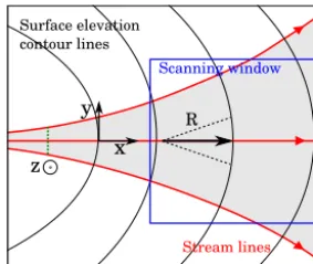
Figure 1.Thexaxis is taken along the ridge stream line, and the
yaxis tangent to the surface elevation contour. The scanning win-dow is used to determine the value ofRin its centre. Lateral stream lines are represented to show the non-linear widening of the flow tube in this particular case, and the corresponding accumulation sur-face is coloured in grey.
Sergienko (2012) showed that the 2-D (x,z) models could not account for the flow of ice on a bumpy bed, because they consider no lateral variability, and recommended using such models on a width-averaged topography. It is however pos-sible to account for variations in the width of the flow tube in the model and still express the equations with (x, z) co-ordinates only (Reeh, 1988); we hereafter call these models 2.5-D models. Under a few flow assumptions (the bed eleva-tion varies slowly in the transverse direceleva-tion, the walls of the flow tube are vertical, and the lateral curvature of the flow-line is small), such models represent an improvement on 2-D models because they account for lateral variability while maintaining the computational speed which full 3-D models lack.
A particularly simple case is that of an axisymmetric cir-cular dome, where the width of the flow tube increases lin-early along the flowline. In any other case, there are several possible methods for determining the width of the flow tube. At a large scale, the ice velocity can be determined via inter-ferometric synthetic-aperture radar data (Rignot et al., 2011), but this is only reliable when ice velocity is large compared to the associated error. In the interior of ice sheets, where the ice velocity is low, velocity measurements can be made using stake monitoring. If correctly positioned, the direction and position of the stakes may give the width of the flow tube (Waddington et al., 2007). Without any available veloc-ity observations, the only possibilveloc-ity is to use a digital el-evation model (DEM) describing the shape of the surface. The velocity measurement method is preferable when pos-sible, since the ice does not always flow perpendicularly to the surface contour lines. However, along a divide, or along the centre line of a drainage basin, the longitudinal surface velocity reaches its minimum or its maximum value com-pared to the lateral surroundings; moreover, if the flowline has a slight horizontal curvature, the horizontal shear strain rate can be neglected (Reeh, 1988). The ice velocity is then
oriented along the steepest surface slope and the curvature of the surface contour lines linked to the width of the flow tube; for a dome or a 2-D ridge, determining the curvature of the surface contour line is sufficient to describe the widening of the flow tube. In this case, to determine the local curvature of a surface, the neighbourhood of each point of a DEM is approximated via interpolation. The size of this neighbour-hood (scanning window) can be freely chosen, but no objec-tive criteria are currently available to make this choice. This approach has been used to compute the surface curvature of an ice sheet (Rémy and Minster, 1997; Rémy et al., 1999), but the size of the scanning window was not discussed. Due to the noise affecting the DEM and due to the regional cur-vature, the local computed curvature may be ambiguous.
The 2-D models that account for the width of the flow tube vary in the complexity of their physics and their underlying assumptions (e.g. Martín et al., 2009; Koutnik and Wadding-ton, 2012; Sergienko, 2012). The 2.5-D model proposed by Reeh (1988) assumes that the streamlines are perpendicular to the surface contour lines (Fig. 1), so that the mass conser-vation equation directly depends on the radius of curvature of the surface contour lines (here calledR). The model im-poses a vertical profile for the horizontal velocity, by the use of a shape function, and the momentum conservation equa-tion was thus not given for any case. This vertical profile is assumed to be unchanging through thex direction (column-flow model). Later on, Hvidberg (1996) improved upon this approach by setting the stress equilibrium equations without any assumption about the shape of the velocity field. Ad-ditionally, when considering a width-varying flow tube, the heat equation should be modified as well, but only a few au-thors have considered this necessary for their purpose (Hvid-berg, 1993, 1996; Pattyn, 2002).
Different authors have used the modelling approach pro-posed by Reeh (1988), or similar ones, at different scales and for various geometries: for example, mountain glacier (Salamatin et al., 2000; Pattyn, 2002), ice-sheet domes (Reeh and Paterson, 1988; Hvidberg et al., 1997a), ice-sheet ridges (Hvidberg et al., 2002) or even for the whole of Greenland (Reeh et al., 2002). The shape and size of the ice bodies are quite diverse, but unfortunately the validity of the 2.5-D ap-proach, and its assumptions, for these different cases has re-ceived little attention. In particular, the transverse deforma-tion of the ice is assumed to be constant through depth (i.e. the walls of the tube are vertical), which may depend on the surface geometry. Furthermore, the error in the computation ofRis only discussed by Hvidberg et al. (1997b), who esti-mated the error in the calculation ofRto be 15 %, and Hvid-berg et al. (2001) by about 50 %. The method used to mea-sureRis not detailed either, and we doubt that its influence is negligible.
as-suming a constant horizontal velocity profile. Furthermore, Reeh (1989) accounted for the spatial evolution ofRwith a simple linear model, based on the surface observation. These considerations suggest that the domain of applicability of 2.5-D models with regards to flow divergence and surface geometry remains to be determined.
As a consequence, the applicability of the 2.5-D model should particularly be examined on dome geometries, where simple 2-D models would be unable to account for flow di-vergence. The flow tubes may widen by several orders of magnitude on a few tens of kilometres, especially on the sharpest ridge of the dome. The goal of this study is to per-form several comparisons between 2.5-D and 3-D models, for various dome geometries and temperature conditions, to answer the following questions.
1. What is the error associated with the computation ofR
from the DEM? This geometric error depends largely on the size of the scanning window.
2. How well can a 3-D state of stress be accounted for by the single parameter R(x)along the flowline? This is related to the inherent error of the 2.5-D model and its underlying assumptions.
To investigate the performance of the 2.5-D model, we com-pare the velocity fields resulting from the 2.5-D and 3-D models, the latter being taken as a reference. To our knowl-edge, no such systematic comparison between the results of 3-D and 2.5-D models has been carried out. As such, we hope the present study will guide future research using 2.5-D models in different scenarios. In the following, we present the equations of the 3-D and 2.5-D models. We then run the simulations on several domes of different shapes: a circu-lar one (axisymmetric), a slightly elongated one, and a very elongated one. We first consider the isothermal case, before moving on to investigate the effects of temperature.
2 Description of the 3-D model
In future work, we hope to investigate a small dome on the East Antarctic plateau. As such, we presently consider a syn-thetic case with similar geometric and thermal conditions. 2.1 Geometry and mesh
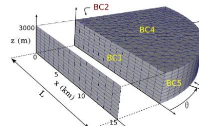
In order to investigate the influence of flow divergence, we model a ridge of a dome, as this results in significant di-vergence. We perform the present model comparison on a synthetic geometry which consists of a 15 km-radius domain, whose shape is a quarter of cylinder only, for reasons of sym-metry. The initial thickness of the ice is 3239 m at the sum-mit, the mean surface slope is around 0.6/1000 and the under-lying bed is flat. The space coordinate is a(x, y, z)Cartesian system.
x (km) z (m)
y
15 0
10 5 3000
BC1 BC4
BC5 BC2
BC3
θ L
Figure 2.View of the two meshes used in this study. For each run, the 2-D mesh is extracted from the geometry of the steady-state so-lution of the 3-D simulation. BC1 to BC5 refer to the five boundary conditions of the 3-D case.
The 3-D mesh is horizontally unstructured and vertically extruded on 10 levels. The horizontal mean spacing between the nodes is 1 km (Fig. 2).
2.2 Mechanical model 2.2.1 Conservation equations
We denote the velocity vectoru, with components(u, v, w)t. The stress and strain rate tensors are denotedσand˙ respec-tively, and their components,σij andij˙ . The deviatoric part ofσis denotedτ, and its components,τij. The 3-D mechan-ical model consists of a Stokes problem for incompressible ice of densityρ, in which the mass and momentum conser-vations equations are written
∇ ·u=0, (1)
∇ ·σ+ρg=0, (2)
wheregis the gravitational acceleration vector. The values of the different parameters are given in Table 1. The ice is assumed to deform following Glen’s generalized flow law (Glen, 1958):
˙
ij=A(T )τen−1τij, (3)
whereτe is the second invariant ofτ. We choose a value of
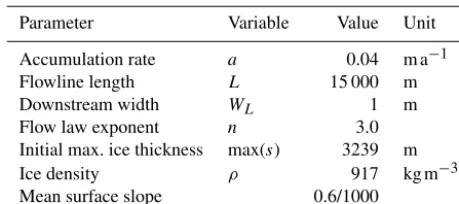
Table 1.Description and values of the model parameters.
Parameter Variable Value Unit
Accumulation rate a 0.04 m a−1
Flowline length L 15 000 m
Downstream width WL 1 m
Flow law exponent n 3.0
Initial max. ice thickness max(s) 3239 m
Ice density ρ 917 kg m−3
Mean surface slope 0.6/1000
respectively. This linear temperature profile is simple but re-alistic enough to show the effect of a warmer ice at the bot-tom. For convenience, and as the bed is flat,b=0 in the fol-lowing experiments.
2.2.2 Boundary conditions
Since the 3-D mesh is a quarter of a cylinder, the conditions have to be set on five different boundaries, numbered from BC1 to BC5 (Fig. 2). We consider frozen ice at the bed and no flow through the lateral boundaries (symmetry condition). Considering no sliding at the bottom and neglecting the at-mospheric pressure at the surface, the boundary conditions are written as follows:
BC1:u.n|y=0=0, (4)
BC2:u.n|x=0=0, (5)
BC3:u|z=0=0, (6)
BC4:σ.n|z=s=0, (7)
wherenis the outward-facing normal vector on the surface. Since the surface (BC4) is let free, a kinematic boundary con-dition for the surfaces(x, y, t )has to be solved as well:
∂s
∂t +u
∂s
∂x+v
∂s
∂y =w+a, (8)
whereais the accumulation rate. The velocity boundary con-dition on BC5 is set to control the shape of the steady-state dome. The method to create an elongated dome is similar to that of Gillet-Chaulet and Hindmarsh (2011), in which the shallow ice approximation is used to prescribe a profile of horizontal velocity at the boundary. As such, BC5 is not a physical boundary, but it allows the domain to be reduced to a reasonable extent. The velocity vector is oriented along the surface slope, and pointing outwards. It is variable with depth to the powern+1 and vanishes at the bed. Its norm is tuned depending on its orientation, so that the shape of the
dome can be elongated in one preferred direction (Fig. 3):
u=ω2 cosθ α
(n+2)
(n+1)×
1−1−z s
(n+1)
, (9)
v=ω2(α−1)sinθ
α
(n+2)
(n+1)×
1−
1−z s
(n+1)
, (10)
whereθis the angle to the edge of the domain, andαa shape parameter controlling the elongation of the dome. The fol-lowing results will correspond to a stabilized steady-state ge-ometry, for a uniform and constant accumulationa in time and space. To do so, the output mean velocityωis tuned to balance the surface accumulation, so that it can be expressed as
ω= a·6
WL·s
, (11)
where6is the surface area of the accumulation zone on the top boundary (grey area in Fig. 1), andWLthe width of the ice flow at the downstream positionx=L. In this particular case, 6 andWL are simply equal to 1/4 of the dome
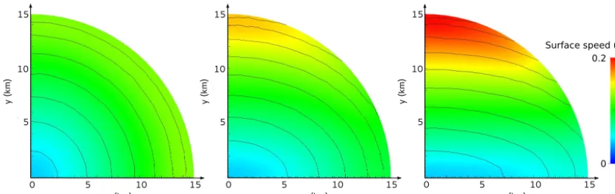
sur-face and dome perimeter, andL is the radius of the dome. Three different values were taken for the shape parameterα: 2 (axisymmetric case, circular geometry), 3, and 6 (Fig. 3). The axisymmetric domain will test the performance of the model for a perfectly known case. The latter two cases will test the ability of the model to account for divergence of vary-ing magnitudes.
3 Description of the 2.5-D model
The coordinate system used by Reeh (1988) is a curvilinear coordinate system with a right-handed oriented coordinate axis. Thex axis is oriented along the flowline, thezaxis is vertically oriented, and they axis is transverse to flow and tangential to a surface contour line. As we only consider here straight flowlines (linear ridge of an ice divide), the coordi-nate system is locally Cartesian (Fig. 1). We refer to the 2.5-D model in the(x, z)coordinate system. We now recall the assumptions made by Hvidberg (1996), partly inherited from Reeh (1988).
1. The flowlines are perpendicular to the surface contour lines.
2. The directions of the horizontal velocity components are constant with depth, which implies that the walls of the flow tube are vertical.
3. There are no shear stresses on the vertical boundaries defined by the flow tube.
4. The ice deforms according to Glen’s flow law.
0 5 10 15 x (km)
5 10 15
y (km
)
Surface speed (m/a)
0 5 10 15 x (km)
0 5 10 15 x (km)
5 10 15
y (km)
5 10 15
y (km)
0.2
0.1
0
Figure 3.The three domes stabilized at steady state: surface contour lines (spacing: 1 m) and surface speed (m a−1) forα=2 (left),α=3 (middle) andα=6 (right).
impose the transverse stresses. Such assumptions are reason-able in the centre of an ice sheet for a slowly varying bed (Reeh, 1988). If the bedrock spatial variations are too steep, they will warp the ice-free surface so that the velocity at the base may not be parallel to the velocity at the surface (Hvid-berg, 1993; Sergienko, 2012).
3.1 Geometry
The 2-D domain is taken as a vertical slice of the 3-D do-main, on one of its lateral boundaries (Fig. 2). The dome be-ing elongated, we will run the 2.5-D model along the sharpest ridge of the 3-D dome (y=0) or perpendicular to it (x=0). 3.2 Mechanical model
We denote the width of the considered flow tubeW (x). The radius of the surface contour linesR(x)is taken as positive for diverging flow and negative for converging flow. In this model, the assumption (2) implies thatWhas no dependence onz, so that geometrical considerations show that W (x)is directly linked toR(x)by
1
R(x)=
1
W (x) ∂W
∂x. (12)
An axisymmetric dome leads to the simple relations
R(x)=x andW (x)∝x. If the flow tube is diverging more
than the axisymmetric flow (on a ridge for example), the cor-responding tube surface is narrowedfor a given output width, and leads to lower output velocities.
The following sections present the equations of mass and momentum conservation, modified to account for the diver-gence of the tube. As the velocity field mainly depends on the input/output balance, some authors only conserve the mass (e.g. Parrenin et al., 2004; Todd and Christoffersen, 2014) but not the momentum; this approach can in particular be sufficient for a vertically integrated model (Hvidberg et al., 1997b). Other authors do not modify the Stokes equations at
all, but instead add an extra-surface mass balance term (Cook et al., 2014; Gladstone et al., 2012) which depends on the divergence of the tube. This approach has the advantage of simplicity and results in a correct output flux, but neglects the true horizontal advection of the ice. However, this can be jus-tified for ice-sheet margins, where the ice mainly undergoes sliding. For all these mass-only conservation models, the nor-mal lateral stress of the surrounding ice is not accounted for, since the force equilibrium is not properly modified. 3.2.1 Mass conservation
At the ice divide, the velocity componentv and its spatial derivatives vanish for reasons of symmetry, so that there is no dependence of the strain rates on the transverse coordi-nate. Under the above assumptions and considering a flow tube of width W (x) (and corresponding radiusR(x)), the normal strain rates in the curvilinear system are then writ-ten as (Jaeger, 1969, p. 45)
˙
xx=
∂u
∂x; ˙yy=
u
R(x); ˙zz=
∂w
∂z. (13)
If the flow tube has a constant width, the value ofR is in-finite and the equation corresponds to the plane strain case. For the more complete form of these expressions, see the dis-cussion of Reeh (1988). The mass conservation then follows:
∂u
∂x+
u
R(x)+
∂w
∂z =0. (14)
3.2.2 Momentum conservation
For a straight flowline, the horizontal shear strain rate is writ-ten as (Reeh, 1988)
˙
xy=
1 2
∂u
∂y −
v
R(x)+
∂v ∂x
. (15)
Along a divide between drainage basins,vvanishes andu
case, there is no horizontal shear strain, and the only non-zero components of strain are the normal ones and the verti-cal strain rate xz˙ . For dome geometries, Hvidberg (1993) shows that the curvilinear coordinate system is equivalent to a cylindrical coordinate system distorted in the y direc-tion, for which the radius of curvature R(x)describes the local distortion. The force equilibrium equations, expressed in the(x, z)Cartesian coordinate system, are inherited from their formulation in cylindrical coordinates, and are written as (Hvidberg, 1996; Jaeger, 1969, p. 123)
∂σxx
∂x +
∂σxz
∂z +
σxx−σyy
R(x) =0, (16)
∂σxz
∂x +
∂σzz
∂z +
σxz
R(x)=ρg, (17)
whereσyyis known in terms ofuandR(x)(Eqs. 3 and 13).
3.2.3 Boundary conditions
The boundary conditions are inherited from the 3-D case: no sliding, free surface, vanishing velocity at the ice divide and an imposed horizontal velocity profile downstream. Note that the value of the mean output velocityωdirectly depends on
6, which is now given by
6=
L Z
0
W (x)dx, (18)
where Lis now the length of the flowline. Equations (11) and (18) together mean that the errors in the calculation of
W result in errors in the prescribed output velocity. Since we consider a straight flowline, there is no transverse flow across the considered plane. The free surface equation is thus derived from Eq. (8), and is equivalent to a simple 2-D case, here given for the(y=0)plane:
∂s
∂t +u
∂s
∂x=w+a. (19)
3.3 Implementation in Elmer/Ice
The modified mechanical equations are implemented in the Elmer/Ice finite element software (Gagliardini et al., 2013). The correct implementation of the mass conservation was checked by comparing different 2.5-D simulations with the Vialov-type profiles (Vialov, 1958) computed for different diverging tubes. The expression of the Vialov profile in the case of a power-law varying flow tube is presented in Ap-pendix A.
3.4 Determination of the contour radius
To determine the radius of curvature of the surface con-tour lines, we first export a DEM from the surface nodes
of the 3-D model. These nodes are fitted using an inverse distance weighting, with a power of 4 in order to ensure a good smoothing of the computed surface, representative of a real ice sheet. For comparability with a real case, the spa-tial resolution of the DEM is taken equal to 400 m, which is the resolution of the DEM resulting from the ICESat mission on Antarctica (Schutz et al., 2005). The DEM surface curva-ture is computed for each pixel, using a scanning window for fitting (Fig. 1). The local surface inside the window is curve-fitted by a bivariate quadratic polynomial function, and the analytical curvature of this function taken as the local cur-vature, which depends on the size of the scanning window used. For example, along an elongated ridge (Fig. 3, middle and right), the surface contours are close to ellipses, but only a sufficiently large scanning window will be able to account for this global shape. A small scanning window may com-pute an approximately circular curvature. By contrast, even though a large window may lead to a more accurate value of the curvature, geometrically speaking, it is not necessarily the case that it will also lead to a more accurate velocity field, since it is difficult to know which surrounding environment is mainly influencing the ice flow. As a consequence, three different sizes of scanning window are tested here, 2.8, 6 and 10 km, thus corresponding to a width of 7, 15 and 25 pixels. For each pixel, the value ofR(x)is taken as the inverse of the curvature of the contours of the fitted surface in the centre of the window. This is done using GRASS GIS software. 3.5 Protocol of comparison
We first run the 3-D transient isothermal simulation, and stop when a steady state is reached (∂s/∂t < 10−6m a−1). We then use the resulting DEM to compute the profile ofRto ini-tialize the 2.5-D model. For each dome configuration (α=2, 3, 6) we compare the different runs chosen: (a) 3-D, (b) 2.5-D for the three scanning windows, and a fixed geometry, (c) 2.5-D for the three scanning windows, with a free surface. For the axi-symmetric case we add a true 2.5-D axisymmetric run (imposing an analytical valueR=x). Then we compare the 3-D and 2.5-D results for non-isothermal ice, to investi-gate the influence of the temperature, especially near the base of the ice sheet.
4 Results and discussion
4.1 Circular geometry (α=2), isothermal ice 4.1.1 3-D/2.5-D axisymmetric comparison
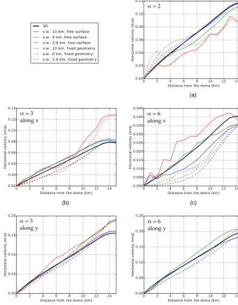
0 2 4 6 8 10 12 14 Dist ance from t he dom e (km ) 0.00 0.02 0.04 0.06 0.08 0.10 0.12 H o ri z o n tal v e loc it y (m /a)
α = 2
0 2 4 6 8 10 12 14
Dist ance from t he dom e (km ) 0.00 0.02 0.04 0.06 0.08 0.10 0.12 0.14 H o ri z o n tal v e loc it y (m /a)
α = 3 along x
0 2 4 6 8 10 12 14 Dist ance from t he dom e (km ) 0.000 0.005 0.010 0.015 0.020 0.025 0.030 0.035 0.040 0.045 H o ri zo n tal v e loc it y (m /a)
α= 6
along x
0 2 4 6 8 10 12 14
Dist ance from t he dom e (km ) 0.00 0.05 0.10 0.15 0.20 H o ri z o n tal v e loc it y (m /a)
α = 3 along y
0 2 4 6 8 10 12 14
Dist ance from t he dom e (km ) 0.00 0.05 0.10 0.15 0.20 0.25 H o ri z o n tal v e loc it y (m /a)
α = 6 along y (d) (e) (c) (b) (a) 3D
s.w.: 10 km , free surface s.w.: 6 km , free surface s.w.: 2.8 km , free surface s.w.: 10 km , fixed geom et ry s.w.: 6 km , fixed geom et ry s.w.: 2.8 km , fixed geom et ry
Figure 4.Horizontal velocity at the ice surface (m a−1) along the flowline, for isothermal ice. Dashed lines are for fixed geometry runs and solid lines for evolved free surface to a steady state. Thick black: 3-D; yellow: 2.5-D axisymmetric (hidden by the black curve); red: 2.5-D scanning window of 2.8 km; green: 2.5-D scanning window of 6 km; blue: 2.5-D scanning window of 10 km.(a)Circular dome,α=2.
(b)α=3, along the ridge.(c)α=6, along the ridge.(d)α=3, perpendicular to the ridge.(e)α=6, perpendicular to the ridge. For this last case, no result concerning the 2.8 km scanning window is shown, since they are completely out of reasonable bounds.
4.1.2 3-D/2.5-D comparison
The computation of the radius of the surface contour lines is strongly influenced by the size of the scanning window. For a circular geometry, the variation of W alongx should be linear, which is almost the case for the two wider windows (Fig. 5, solid lines). With this regular geometry, the larger the window, the more precise the radius, since the fitted surface will be more accurate. By contrast, the width value computed with the smaller window is less regular and underestimated
by about 30 %, meaning that we cannot evaluate a certain cur-vature from too small a sample. When choosing the interme-diate or larger scanning window, the root mean square error (RMSE) in the velocity is 9.9 or 3.1 % respectively (Fig. 4a), and is a consequence of the error in the calculation of the radius.
Figure 5.Relative width of the flow tubeWfor the different dome geometries: circular (α=2, solid lines), slightly elongated (α=3, dashed lines) and very elongated (α=6, dotted lines); for differ-ent scanning windows: 2.8 km (red), 6 km (green) and 10 km (blue). The yellow curve is the line for whichR=xis imposed (axisym-metric case).
4.2.1 3-D/2.5-D comparison, along the ridge
Along a ridge, the flow tube is non-linearly diverging. For a given output width, the accumulation area is smaller than in the axisymmetric case, thus leading to lower output veloci-ties.
With fixed geometries, it clearly appears that the velocity is underestimated for elongated domes (Fig. 4b and c, dashed lines), meaning that the local surface slope cannot explain the ice motion by itself: the ice along the ridge is also, if not mainly, pulled by the surrounding lateral ice, which moves due to a steeper surface slope. The case of the small scanning window appears to be different (Fig. 4b, red dashed line), simply because of a really poor estimation ofW, and thus of the output velocity.
The downstream velocities are always quite accurate (10 % error), since they mainly depend on the tube surface calculation, incorporated into the velocity boundary condi-tion. When releasing the surface, the surface slope slightly increases to accommodate the velocity boundary condition, and the computed velocity field is then closer to the 3-D ref-erence. The relative error made in the downstream part of the flow is comparatively higher near the divide since the veloc-ities are very small.
In the case of a sharp ridge, the ice surface has the shape of a circus tent (Fig. 6, dotted line), i.e. the ice slope increases when going towards the divide. This shape is clearly not physical, and is the result of a numerical artefact. Since the vertical strain rate is always of the order ofa/H, the conser-vation equation leads to a balance between∂u/∂xandu/R
close to the divide. For highly diverging flows,u/Ris much smaller than for an axisymmetric case at the samexposition (Appendix B). As a consequence,∂u/∂xshould have a
com-Figure 6.Height of the ice surface (m) for the 2.5-D free surface model, along the ridge. Solid line: circular geometry,α=2. Dashed line:α=3. Dotted line:α=6.
paratively much higher value. The only way foruto increase over a short distance near the divide is for the surface eleva-tion to decrease sharply. To handle this artefact, we increased the mesh resolution near the dome, but without any success-ful results. This artefact does not appear forα=3 (slightly elongated dome).
Forα=6, the tube surface is better estimated with an in-termediate window, whose size is closer to the local value ofR. The RMSE in the velocity is 12.1 % for the interme-diate window and 44.3 % for the large window. Too large a window would consider the whole shape of the dome and lead to an underestimation of R. The amplitude of the er-ror between the different runs shows that for sharp ridges (or highly diverging tubes) the choice of the window size is not straightforward, as a wider window increases the regularity of the velocity field, but decreases the ability to capture the local curvature.
Reeh (1989), using a 2.5-D model for dating purposes, explained the large errors for the diverging tube of Camp Century partly by the simplicity of his model, especially his linear model ofR. The computed velocities show important discrepancy with the oberved ones, which leads to a bad esti-mation of the origin position of the ice, by 200 %. The error made in the velocity field with this more complete model seems now to be small enough for tracking ice particles cor-rectly, for example with the intermediate window size. How-ever, for a real case of highly curved surface, it is difficult to know a priori the best window size to use and whether the divergence can be properly accounted for, in the absence of a reference as is done here.
0 5000 10 000 15 000 x (m )
0 500 1000 1500 2000 2500 3000
z (
m
)
0 5000 10 000 15 000
x (m ) 0
500 1000 1500 2000 2500 3000
z (
m
)
0.00 0.04 0.08
Horizont al speed (m /a)
0 5000 10 000 15 000
x (m ) 0
500 1000 1500 2000 2500 3000
z (
m
)
0 5000 10 000 15 000
x (m ) 0
500 1000 1500 2000 2500 3000
z (
m
)
Figure 7.Horizontal velocity field (m a−1), for the non-isothermal case andα=3. Top: 3-D model. Bottom: 2.5-D model, with a scanning window of 10 km. Left:α=3, white contour lines spaced by 0.01 m a−1. Right:α=6, white contour lines spaced by 0.005 m a−1.
and large window size respectively, forα=3, and 13.7 and 11.1 % forα=6; this error is slightly higher than for the cir-cular geometry (Fig. 4d). In the case of large radius values, towards the exterior of the dome, the wider window gives the more accurate results.
4.3 Non-isothermal ice
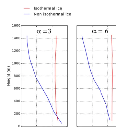
A supplementary comparison is carried out on the sharp ridge (y=0) for temperature varying linearly through depth. The computed velocity field towards the divide (low x values) shows a reversed vertical profile, i.e. the basal ice goes faster than the upper ice (Fig. 7, bottom). This non-physical result in 2.5-D can be explained this way: as soon as a 3-D tube diverges more than for an axisymmetric flow, the warmer basal ice is more easily laterally strained than the colder sur-face ice. As a consequence, the walls of the 3-D flow tube are no longer vertical, and using the 2.5-D model in such a case would violate assumption (2). This effect is particularly pronounced close to the divide, where the tube is narrower, and can be seen in the 3-D simulations as follows (Fig. 8). The stream lines going through a flux gate at x=1000 m are tracked on a few hundred metres (x=1200 m forα=6,
x=1500 m forα=3). The divergence of the stream lines depends on their depth – the tube is larger near the bottom (Fig. 8, blue curves) – and this dependence is stronger for high diverging tubes. To accommodate the lateral strain in this case, the 2.5-D model computes high horizontal veloci-ties in the bottom, whereas the real motion is in fact mainly laterally oriented. No mesh refinement has been able to cor-rect this problem. Since it does not happen for a constant temperature, it certainly originates from the lower viscosity of the basal ice (Fig. 8, red curves).
250 260 270
Widt h of t he t ube (m )
0 200 400 600 800 1000 1200 1400 1600
H
e
ight
(
m
)
320 360 400 440
Widt h of t he t ube (m )
α= 6
α= 3 Isot herm al ice Non isot herm al ice
Figure 8.Width of the flow tube (m), for the isothermal (red) and non-isothermal case (blue), forα=3 (x=1500 m, left) andα=6 (x=1200 m, right). The aspect of the curves is slightly affected by numerical noise due to discretization.
the sharpest far from the summit, whereas it is the contrary in our case. The artefact that appears in our simulations may not be as sensitive in their case. Nevertheless, care must be taken in such cases, since the basic assumptions may not be justifiable and the model is likely to be outwith its application domain.
For reasons of continuity, the walls of the flow tube cannot be vertical in the direction perpendicular to the ridge either, but the effect is too weak to impact the computed velocity field.
5 Conclusions
A systematic comparison between 2.5-D and 3-D models has been presented in order to evaluate the ability of the former to accurately compute the velocity field on a small dome of an ice sheet. The error made when estimating the value of the ra-dius of the surface contour lines is of the order of 10 % if the computation window is well chosen, though it can be com-paratively higher close to the divide. The radius of curvature of the surface elevation contour lines should be determined with a sufficiently large computation window, but choosing the optimum size is not completely straightforward; in any case we suggest it should not be less than one-third of the maximum measured radius, and several windows should be tested to ensure the robustness of the results.
The 2.5-D model can be used without any specific restric-tion for tubes diverging less than and up to an axisymmetric flow. For isothermal ice, the model can be used with tubes di-verging more than an axisymmetric flow, if the divergence is not too high. For very high divergence, the ice is in our study mainly pulled by the output boundary condition, and the re-sulted velocity field may be somewhat irregular, and surface geometry unphysical close to the divide. This means that, in the case of a sharp ridge, accounting for a certain state of stress via a single parameterR(x)is clearly not possible. In practice, the examples of surface topographies given in this study may serve as a reference to evaluate whether using a 2.5-D model for a real case is justifiable.
For non-isothermal ice, the tube should not diverge more than axisymmetry, because the softer basal ice would be
much more easily laterally strained in the case of an elon-gated dome. The walls of the flow tube are therefore not ver-tical, which violates the model assumptions, and the corre-sponding horizontal velocity profile may be not physical near the divide. This has significant consequences for dating pur-poses: as the computed velocity field shows too small values in the upper layers, the age of the ice is overestimated, and the modelled isochrone layers are too high. In the absence of a reference 3-D solution as produced here, the velocity field may not necessarily appear to be unphysical, but this does not mean that the numerical artefact does not significantly affect the age calculation.
This study shows that the use of a 2.5-D model, which is a trade-off between 2-D and 3-D, must avoid several pit-falls, and its applicability domain appears to be significantly narrower than initially thought. The geometric error, result-ing from miscalculation ofR, should have less impact on the quality of the results than the inherent errors related to the violation of the 2.5-D model’s assumptions, especially when the temperature varies through the ice column. The 2.5-D model was designed for divides between drainage basins, but real flowlines along sharp divides should not be modelled this way. Finally, for a real case, it has not been established how flat the bedrock should be to ensure that the assumption of verticality of the walls of the flow tube is reasonably re-spected, even for a slightly divergent flow. The applicability domain of the 2.5-D model for slightly horizontally curved flowlines has not been investigated here, but further uncer-tainties are expected in this case, for which some second-order terms are neglected in the mass conservation.
6 Code availability
Appendix A: Vialov profile for a power-law diverging tube
To check the correct implementation of the mass conserva-tion in the 2.5-D model, we hereafter compute the height of a Vialov profile corresponding to a regularly diverging flow tube. Note that such a surface is only representative of a sin-gle flowline, and not of a whole surface, as is usually done for a Vialov profile in plane strain (Vialov, 1958) or axisym-metry (Ritz, 1992).
Figure 5 shows that we may approximate the shape of the flow tube by a power law depending on thexcoordinate. Let consider a flow tube of widthW=WL Lx
β
. For plane flow,
β=0, for axisymmetry,β=1, and for sharp ridges,β >1. The volume outflow q∗ for a certain coordinatex may be expressed in one of two ways (Cuffey and Paterson, 2010, p. 388):
q∗=
x Z
0
a
x0
L
β
WLdx0=
ax
(β+1)
x
L
β
WL
= axW
(β+1), (A1)
q∗=
2A
n+2τ
n
bH
H W, (A2)
whereH is the ice thickness,τbthe basal shear,athe accu-mulation rate,Lthe length of the glacier, andAthe rate fac-tor of Glen’s flow law. Equating the two expressions yields
a·x=2A(β+1)
n+2 τ
n
bH
2. (A3)
The following reasoning is then similar to that of Cuffey and Paterson (2010), simply modified by a(β+1)multiplier. The final expression for the ice thickness is unchanged:
H=H∗
1−x L
n+n1
n
2n+2
, (A4)
except for the height of the ice sheetH∗at the dome (x=0), which is now
H∗=
2(n+2)1/n ρg
2nn+2√
L
a
2A(β+1)
2n1+2
. (A5)
This expression is consistent with the one previously de-rived for axisymmetry. We then use this expression to control the 2.5-D model by comparing the value ofH∗computed by the model with its above theoretical value.
Appendix B: Radius and surface of a power-law diverging flow tube
We consider the same flow as in Appendix A. The value of the radiusR(x)is then expressed as
1
R(x)=
1
W
dW
dx =
d ln(W )
dx = β
x. (B1)
The surface area of the tube upstream ofxcan be expressed as
6(x)=
x Z
0
W (x)dx= WL
β+1
xβ+1
Lβ . (B2)
As u is more or less proportional to the upstream sur-face area6,u/Ris expected to be proportional toWL xLβ. On the contrary, one can consider that the value of∂u/∂x
should be of the order of ω/L, i.e. simply proportional to
6(L)/L=WL/(β+1). Near the divide,u/Ris then
Author contributions. The experiments were designed by Olivier Gagliardini, Frédéric Parrenin and Joe Todd. Olivier Pas-salacqua carried them out, helped by Catherine Ritz for analytical developments, and by Fabien Gillet-Chaulet for the Elmer/Ice implementation. Olivier Passalacqua prepared the manuscript with contributions from all co-authors.
Acknowledgements. We would like to thank the Editor D. Gold-berg as well as D. Brinkerhoff and an anonymous referee for their frank comments which greatly improved the initial version of the manuscript. This project is supported by the Université Grenoble Alpes in the framework of the proposal called Grenoble Innovation Recherche AGIR.
Edited by: D. Goldberg
References
Cook, S., Rutt, I. C., Murray, T., Luckman, A., Zwinger, T., Selmes, N., Goldsack, A., and James, T. D.: Modelling environmental in-fluences on calving at Helheim Glacier in eastern Greenland, The Cryosphere, 8, 827–841, doi:10.5194/tc-8-827-2014, 2014. Cuffey, K. M. and Paterson, W. S. B.: The physics of glaciers,
Aca-demic Press, Burlington, Massachusetts, USA, 2010.
Gagliardini, O., Zwinger, T., Gillet-Chaulet, F., Durand, G., Favier, L., de Fleurian, B., Greve, R., Malinen, M., Martín, C., Råback, P., Ruokolainen, J., Sacchettini, M., Schäfer, M., Seddik, H., and Thies, J.: Capabilities and performance of Elmer/Ice, a new-generation ice sheet model, Geosci. Model Dev., 6, 1299–1318, doi:10.5194/gmd-6-1299-2013, 2013.
Gillet-Chaulet, F. and Hindmarsh, R. C. A.: Flow at ice-divide triple junctions: 1. Three-dimensional full-Stokes modeling, J. Geophys. Res.-Earth, 116, F02023, doi:10.1029/2009JF001611, 2011.
Gillet-Chaulet, F., Gagliardini, O., Seddik, H., Nodet, M., Du-rand, G., Ritz, C., Zwinger, T., Greve, R., and Vaughan, D. G.: Greenland ice sheet contribution to sea-level rise from a new-generation ice-sheet model, The Cryosphere, 6, 1561–1576, doi:10.5194/tc-6-1561-2012, 2012.
Gladstone, R. M., Lee, V., Rougier, J., Payne, A. J., Hellmer, H., Le Brocq, A., Shepherd, A., Edwards, T. L., Gregory, J., and Cornford, S. L.: Calibrated prediction of Pine Island Glacier retreat during the 21st and 22nd centuries with a cou-pled flowline model, Earth Planet. Sc. Lett., 333, 191–199, doi:10.1016/j.epsl.2012.04.022, 2012.
Glen, J.: The flow law of ice: A discussion of the assumptions made in glacier theory, their experimental foundations and con-sequences, IASH Publ., 47, 171–183, 1958.
Hvidberg, C. S.: A thermo-mechanical ice flow model for the centre of large ice sheets, PhD thesis, University of Copenhagen, 1993. Hvidberg, C. S.: Steady-state thermomechanical modelling of ice flow near the centre of large ice sheets with the finite-element technique, Ann. Glaciol., 23, 116–123, 1996.
Hvidberg, C. S., Dahl-Jensen, D., and Waddington, E.: Ice flow be-tween the Greenland Ice Core Project and Greenland Ice Sheet Project 2 boreholes in central Greenland, J. Geophys. Res.-Oceans, 102, 26851–26859, doi:10.1029/97JC00268, 1997a.
Hvidberg, C. S., Keller, K., Gundestrup, N. S., Tscherning, C. C., and Forsberg, R.: Mass balance and surface movement of the Greenland Ice Sheet at Summit, Central Greenland, Geophys. Res. Lett., 24, 2307–2310, doi:10.1029/97GL02280, 1997b. Hvidberg, C. S., Keller, K., Gundestrup, N., and Jonsson,
P.: Ice-divide flow at Hans Tausen Iskappe, North Green-land, from surface movement data, J. Glaciol., 47, 78–84, doi:10.3189/172756501781832485, 2001.
Hvidberg, C. S., Keller, K., and Gundestrup, N. S.: Mass bal-ance and ice flow along the north-northwest ridge of the Green-land ice sheet at NorthGRIP, Ann. Glaciol., 35, 521–526, doi:10.3189/172756402781816500, 2002.
Jaeger, J.: Elasticity, Fracture and Flow, with Engineering and Geo-logical Applications, Methuen, London, 268 pp., 1969. Koutnik, M. R. and Waddington, E. D.: Well-posed boundary
con-ditions for limited-domain models of transient ice flow near an ice divide, J. Glaciol., 58, 1008–1020, 2012.
Martín, C., Hindmarsh, R. C., and Navarro, F. J.: On the ef-fects of divide migration, along-ridge flow, and basal sliding on isochrones near an ice divide, J. Geophys. Res.-Earth, 114, F02006, doi:10.1029/2008JF001025, 2009.
Martín, C., Hindmarsh, R. C. A., and Navarro, F. J.: Dating ice flow change near the flow divide at Roosevelt Island, Antarctica, by using a thermomechanical model to predict radar stratigraphy, J. Geophys. Res.-Earth, 111, F01011, doi:10.1029/2005JF000326, 2006.
Parrenin, F., Rémy, F., Ritz, C., Siegert, M. J., and Jouzel, J.: New modeling of the Vostok ice flow line and implication for the glaciological chronology of the Vostok ice core, J. Geophys. Res.-Atmos., 109, D20102, doi:10.1029/2004JD004561, 2004. Pattyn, F.: Transient glacier response with a higher-order
numerical ice-flow model, J. Glaciol., 48, 467–477, doi:10.3189/172756502781831278, 2002.
Reeh, N.: A flow-line model for calculating the surface profile and the velocity, strain-rate, and stress fields in an ice sheet, J. Glaciol., 34, 46–54, 1988.
Reeh, N.: The age-depth profile in the upper part of a steady-state ice sheet, J. Glaciol., 35, 406–417, 1989.
Reeh, N. and Paterson, W.: Application of a flow model to the ice-divide region of Devon Island ice cap, Canada, J. Glaciol., 34, 55–63, 1988.
Reeh, N., Oerter, H., and Thomsen, H. H.: Comparison be-tween Greenland ice-margin and ice-core oxygen-18 records, Ann. Glaciol., 35, 136–144, doi:10.3189/172756402781817365, 2002.
Rémy, F. and Minster, J.-F.: Antarctica Ice Sheet Curvature and its relation with ice flow and boundary conditions, Geophys. Res. Lett., 24, 1039–1042, doi:10.1029/97GL00959, 1997.
Rémy, F., Shaeffer, P., and Legrésy, B.: Ice flow physical processes derived from the ERS-1 high-resolution map of the Antarctica and Greenland ice sheets, Geophys. J. Int., 139, 645–656, 1999. Rignot, E., Mouginot, J., and Scheuchl, B.: Ice Flow
of the Antarctic Ice Sheet, Science, 333, 1427–1430, doi:10.1126/science.1208336, 2011.
Salamatin, A. N., Murav’yev, Y. D., Shiraiwa, T., and Matsuoka, K.: Modelling dynamics of glaciers in volcanic craters, J. Glaciol., 46, 177–187, doi:10.3189/172756500781832990, 2000. Schutz, B., Zwally, H., Shuman, C., Hancock, D., and DiMarzio,
J.: Overview of the ICESat mission, Geophys. Res. Lett., 32, L21S01, doi:10.1029/2005GL024009, 2005.
Sergienko, O.: The effects of transverse bed topography varia-tions in ice-flow models, J. Geophys. Res.-Earth, 117, F03011, doi:10.1029/2011JF002203, 2012.
Todd, J. and Christoffersen, P.: Are seasonal calving dynamics forced by buttressing from ice mélange or undercutting by melt-ing? Outcomes from full-Stokes simulations of Store Glacier, West Greenland, The Cryosphere, 8, 2353–2365, doi:10.5194/tc-8-2353-2014, 2014.
Vialov, S.: Regularities of glacial shields movement and the theory of plastic viscous flow, Physics of the movements of ice IAHS, 47, 266–275, 1958.