Description and evaluation of the Community Multiscale Air Quality (CMAQ) modeling system version 5.1

(1)

www.geosci-model-dev.net/10/1703/2017/ doi:10.5194/gmd-10-1703-2017

Description and evaluation of the Community Multiscale Air

Quality (CMAQ) modeling system version 5.1

K. Wyat Appel1, Sergey L. Napelenok1, Kristen M. Foley1, Havala O. T. Pye1, Christian Hogrefe1,

Deborah J. Luecken1, Jesse O. Bash1, Shawn J. Roselle1, Jonathan E. Pleim1, Hosein Foroutan1, William T. Hutzell1, George A. Pouliot1, Golam Sarwar1, Kathleen M. Fahey1, Brett Gantt2, Robert C. Gilliam1, Nicholas K. Heath1, Daiwen Kang1, Rohit Mathur1, Donna B. Schwede1, Tanya L. Spero3, David C. Wong1, and Jeffrey O. Young1

1_{Computational Exposure Division, National Exposure Research Laboratory, Office of Research and Development,}

US Environmental Protection Agency, Research Triangle Park, NC, USA

2_{Air Quality Analysis Division, Office of Air Quality Planning and Standards, Office of Air and Radiation,}

3_{Systems Exposure Division, National Exposure Research Laboratory, Office of Research and Development,}

Correspondence to:K. Wyat Appel ([email protected]) Received: 31 August 2016 – Discussion started: 7 September 2016

Revised: 17 February 2017 – Accepted: 27 March 2017 – Published: 21 April 2017

Abstract.The Community Multiscale Air Quality (CMAQ) model is a comprehensive multipollutant air quality model-ing system developed and maintained by the US Environ-mental Protection Agency’s (EPA) Office of Research and Development (ORD). Recently, version 5.1 of the CMAQ model (v5.1) was released to the public, incorporating a large number of science updates and extended capabilities over the previous release version of the model (v5.0.2). These updates include the following: improvements in the meteorological calculations in both CMAQ and the Weather Research and Forecast (WRF) model used to provide meteorological fields to CMAQ, updates to the gas and aerosol chemistry, revi-sions to the calculations of clouds and photolysis, and im-provements to the dry and wet deposition in the model. Sen-sitivity simulations isolating several of the major updates to the modeling system show that changes to the meteorological calculations result in enhanced afternoon and early evening mixing in the model, periods when the model historically un-derestimates mixing. This enhanced mixing results in higher ozone (O3) mixing ratios on average due to reduced NO

titra-tion, and lower fine particulate matter (PM2.5) concentrations

due to greater dilution of primary pollutants (e.g., elemental and organic carbon). Updates to the clouds and photolysis calculations greatly improve consistency between the WRF and CMAQ models and result in generally higher O3mixing

ratios, primarily due to reduced cloudiness and attenuation of photolysis in the model. Updates to the aerosol chemistry result in higher secondary organic aerosol (SOA) concentra-tions in the summer, thereby reducing summertime PM2.5

bias (PM2.5 is typically underestimated by CMAQ in the

summer), while updates to the gas chemistry result in slightly higher O3and PM2.5on average in January and July. Overall,

the seasonal variation in simulated PM2.5generally improves

in CMAQv5.1 (when considering all model updates), as sim-ulated PM2.5 concentrations decrease in the winter (when

PM2.5 is generally overestimated by CMAQ) and increase

in the summer (when PM2.5is generally underestimated by

CMAQ). Ozone mixing ratios are higher on average with v5.1 vs. v5.0.2, resulting in higher O3mean bias, as O3tends

to be overestimated by CMAQ throughout most of the year (especially at locations where the observed O3is low);

how-ever, O3correlation is largely improved with v5.1. Sensitivity

simulations for several hypothetical emission reduction sce-narios show that v5.1 tends to be slightly more responsive to reductions in NOx(NO+NO2), VOC and SOx(SO2+SO4)

emissions than v5.0.2, representing an improvement as pre-vious studies have shown CMAQ to underestimate the ob-served reduction in O3 due to large, widespread reductions

(2)

1704 K. W. Appel et al.: CMAQv5.1 description and evaluation 1 Introduction

Numerous federal (e.g., United States Environmental Protec-tion Agency, USEPA), state and private entities rely on nu-merical model simulations of atmospheric chemistry, trans-port and deposition of airborne emissions as well as the re-sulting pollutants as part of their decision-making process for air quality management and mitigation (e.g., Scheffe et al., 2007). Chemical transport models (CTMs), such as the Community Multiscale Air Quality (CMAQ) model (Byun and Schere, 2006), are often employed to provide informa-tion about the potential effects of emission control strategies (e.g., Fann et al., 2009) and climate change (e.g., Nolte et al., 2008), and to provide next-day air quality forecasts (e.g., Eder et al., 2006) in order to inform and protect the pub-lic from potentially harmful air pollutants. Since these mod-els are often used to inform the standard setting and imple-mentation for criteria pollutants (e.g., ozone (O3) and fine

particulate matter (PM2.5)), they must be maintained at the

state-of-the-science level. New versions of the CMAQ model have been released periodically over the past 15 years, with each new version consisting of numerous updates to the sci-entific algorithms within the model, while also improving the quality of the input data used. Collectively, these updates are aimed at improving the underlying science of atmospheric dynamics and chemistry represented in the model, extending the capabilities for emerging applications, and reducing sys-tematic biases in the modeling system. Every new release of the CMAQ model undergoes extensive evaluation in order to establish its credibility (e.g., Mebust et al., 2003; Appel et al., 2007, 2008, 2013; Foley et al., 2010) and documents its performance relative to previous versions. Most recently, the CMAQ modeling system version 5.1 (v5.1) has been tested and evaluated against observations and was publicly released in December 2015 (http://www.cmaq-model.org/).

The scientific upgrades in the CMAQv5.1 modeling sys-tem include major revisions to the Pleim–Xiu land-surface model (PX-LSM; Pleim and Xiu, 1995) and the asymmet-ric convective mixing version 2 (ACM2; Pleim, 2007a, b) planetary boundary layer (PBL) model in the Weather Re-search And Forecast (WRF) model version 3.7 (Skamarock et al., 2008), which required revisions to the ACM2 scheme in CMAQ to maintain consistency. Corrections were also made to the Monin–Obukhov length (MOL) calculation in CMAQv5.1 to make it consistent with the calculation in the WRF model. The changes to the PX-LSM, ACM2 and MOL calculations in CMAQ had significant impact on the mixing within both WRF and CMAQ, and hence large impacts on the pollutant concentrations in CMAQ. These updates are de-scribed in Sect. 2.1. A new explicit treatment of secondary organic aerosol (SOA) formation from isoprene, alkenes and polycyclic aromatic hydrocarbons (PAHs) was also added in CMAQv5.1. Additionally, two aerosol mechanisms are now available in v5.1, AERO6 and AERO6i (with isoprene exten-sions), which include updates to the SOA and ISORROPIA

algorithms (Nenes et al., 1998, 1999). The AERO5 mech-anism has been deprecated and is no longer available. The updates to the aerosol treatment in v5.1 are described in Sect. 2.2. Significant changes were also made to the in-line calculation of photolysis rates (described in Sect. 2.3). The photochemistry in v5.1 underwent major changes; specifi-cally, the photochemical cross sections and quantum yields for the carbon bond 2005 e51 (CB05e51) chemical mech-anism were updated, along with updates to inorganic and organic chemical reaction rates and products to ensure con-sistency with the International Union of Pure and Applied Chemistry (IUPAC). Finally, the representation of organic ni-trate species in CB05e51 was added. These updates are de-scribed in Sect. 2.4.

Section 2 provides a brief description of the major sci-entific and structural improvements included in v5.1. The model configuration and observational data sets used in the model evaluation are provided in Sect. 3. The evaluation of v5.1 is then presented in two parts. Section 4 documents the evaluation of several specific changes that were isolated as part of the overall testing of the model. Specifically, Sect. 4.1 evaluates the meteorological updates in WRF and CMAQ; Sect. 4.2 evaluates the aerosol updates; Sect. 4.3 evaluates the changes to the inline photolysis calculation and the rep-resentation of clouds within CMAQv5.1; and Sect. 4.4 evalu-ates the updevalu-ates to the CB05e51 chemical mechanism. These increments were chosen as the focus of this paper because they represent a fundamental change from the previously re-leased model version and had the propensity to impact model performance for criteria pollutants. The second portion of the evaluation, presented in Sect. 5, summarizes the over-all change in PM2.5 and O3 model performance with v5.1

compared to the previously released version (CMAQ version 5.0.2: v5.0.2). Section 6 provides a discussion of the model response of O3and PM2.5to hypothetical reductions in

emis-sions. Finally a summary discussion in provided in Sect. 7.

(3)

the “major” updates made to the CMAQ modeling system from the previous model version, and therefore do not con-stitute a fully comprehensive description of all the changes made to the system. This section briefly describes these “ma-jor” updates to CMAQ, providing the reader with an under-standing of what was updated in the model and why. A com-prehensive description of all the updates made in v5.1 and in-depth technical documentation of those changes can be found on the CMAS Center website for the CMAQv5.1 release at https://cmaswiki-cempd.vipapps.unc.edu/index.php/. 2.1 WRF and CMAQ meteorological and transport

updates

The WRF and CMAQ models were updated to improve the representation of land-surface processes and vertical mixing. There were two changes made to the PX-LSM in WRF. First, the stomatal conductance function for photosynthetically ac-tive radiation (PAR) was revised based on measurements of net photosynthetic rate as a function of PAR for cotton plants, reported by Echer and Rosolem (2015). The new functions yield a significantly lower magnitude when shortwave radi-ation is less than 350 W m−2. This in turn results in reduced latent heat flux and enhanced sensible heat flux, causing a de-lay in surface stabilization (prolongs mixing) during evening transition hours (i.e., sunset). This reduces overestimations (reduced positive bias) in water vapor mixing ratios, which are common in the WRF–CMAQ modeling system during the evening transition. Similarly, overestimation of concen-trations of surface-emitted species (e.g., NO, NO2, CO and

elemental carbon (EC)) are also reduced during the evening transition. This change was released in WRFv3.7 and fur-ther revised in WRFv3.8. The second change made to the PX-LSM is an increase of the coefficient to the surface en-ergy forcing in the soil temperature force-restore equation (Cv), which is related to volumetric heat capacity (cv) and

heat conductivity (λ) (Pleim and Gilliam 2009) as follows:

Cv=2

π cvλτ

1₂

, (1)

where τ is 1 day (86 400 s), from the previous value of 8×10−6K m2J−1recommended by Giard and Bazile (2000) to 1.2×10−5K m2J−1. The new value forCvresults from

updated values forcvandλor vegetation based on

measure-ments of various leaves by Jayakshmy and Philip (2010) (cv

= 2.0×106J m−3K−1,λ=0.5 W m−1K−1). These changes reduce overestimations of minimum 2 m temperature (i.e., warmer surface temperatures) during the early morning (dawn) hours while also reducing underestimations of 2 m temperature during the post-dawn hours.

There were also two major revisions made to the ACM2 vertical mixing scheme in both WRF and CMAQ. In WRF, the ACM2 was updated to estimate and apply different eddy diffusivities for momentum (Km) and heat (Kh) so that the

Prandtl number (Pr) is no longer assumed to be unity (Pr=

Km/Kh6=1). The second major modification to ACM2 is

the implementation of new stability functions for both heat and momentum for stable conditions, which allows for more mixing in the stable regimes, particularly moderately sta-ble conditions that often occur in the early evening hours. CMAQv5.1 has also been modified to include the same sta-bility functions that are used in WRFv3.7, and therefore, for consistency, WRFv3.7 (or newer) and CMAQv5.1 should be used together. Both of these revisions to the ACM2 are de-scribed in Pleim et al. (2016).

The MOL values used in the ACM2 model in CMAQ were found to differ from the MOL values used in the ACM2 model in WRF. Specifically, the output from WRF was for a preliminary estimate of MOL that was computed in the sur-face layer model in WRF (module_sf_pxsfclay.F). The MOL was later re-computed in ACM2 in WRF but not loaded into the output array. This inconsistency has been fixed in v5.1 by re-computing the MOL in CMAQ exactly as it is computed in ACM2 in WRF. However, starting with WRFv3.8, this re-computed MOL value will be available in the WRF output, and therefore it will be unnecessary to re-compute the MOL value in CMAQ.

2.2 Scientific improvements in the CMAQv5.1 aerosol treatment

CMAQ has historically underestimated SOA in both urban (Woody et al., 2016) and rural (Pye et al., 2015) locations. Thus, improvements to the representation of aerosol from anthropogenic and biogenic hydrocarbons were needed. The updates to SOA formed from anthropogenic volatile organic compounds (VOCs) focus on VOCs in existing emission in-ventories, such as the EPA National Emissions Inventory (NEI), that are likely to fall in the intermediate VOC (IVOC) range. These include long-chain alkanes such as heptadecane and PAHs such as naphthalene. Since these compounds are much less volatile than traditional VOCs, they readily form aerosol in high yields. Long-chain alkanes and PAHs were included in other VOC categories in CMAQ versions prior to v5.1, but were lumped with smaller, more-volatile com-pounds that did not form SOA with the same efficiency. By separating long-chain alkanes and naphthalene at the emis-sion processing step, CMAQ can better account for their higher yields. Several studies (e.g., Pye and Pouliot, 2012; Jathar et al., 2014) have indicated that a large fraction of VOC emissions, particularly IVOC-type compounds, may not be characterized in emission inventories, which limits how much SOA can be formed from anthropogenic VOCs in current CTMs.

(4)

1706 K. W. Appel et al.: CMAQv5.1 description and evaluation

Table 1.New and revised SOA species in the CMAQv5.1 AERO6 mechanism.

Aerosol species Change since v5.0.2 Applicable mechanism Description of modification

AH3OP added all Hydronium ion (predicted by ISORROPIA for

I+J modes); used for IEPOX uptake

APAH1,2 added cb05e51, saprc07tb, saprc07tc,

saprc07tic, racm

Naphthalene aerosol from RO2+NO reactions

APAH3 added cb05e51, saprc07tb, saprc07tc,

saprc07tic, racm

Naphthalene aerosol from RO2+HO2

reac-tions

AISO1,2 updated cb05e51, saprc07tb, saprc07tc∗, racm Aerosol from isoprene reactions NO3added to

existing OH (all yields follow the OH pathway)

AISO3 updated cb05e51, saprc07tb, saprc07tc∗, racm Aerosol from reactive uptake of IEPOX on aqueous aerosol particles. Specifically intended to be the sum of 2-methyltetrols and IEPOX-derived organosulfates

AALK1,2 added cb05e51, saprc07tb, saprc07tc,

saprc07tic, racm

Alkane aerosol

AALK removed all Deprecated alkane aerosol

∗_{AERO6i does not include SOA from isoprene}₊_NO

3in AISO1,2 (it is included in AISOPNNJ). AERO6i does not include IEPOX SOA in AISO3 (it is included in AITETJ,

AIEOSJ, AIDIMJ, etc.). AISO3 is approximately zero in AERO6i.

areas. Naphthalene oxidation is predicted to produce more modest amounts of SOA (Pye and Pouliot, 2012). Note that PAH SOA in v5.1 only considers naphthalene as the parent hydrocarbon, which is about half of the PAHs considered as SOA precursors in Pye and Pouliot (2012). This approach was used since naphthalene is a high-priority hazardous air pollutant (HAP) and necessary in the model for purposes other than SOA formation.

CMAQv5.1 has been updated to include the isoprene epoxydiol (IEPOX) SOA resulting from aqueous reac-tions for most chemical mechanisms including CB05 and SAPRC07, as described in Pye et al. (2013). Later-generation isoprene oxidation products formed under low-NOx

condi-tions, specifically IEPOX, are recognized as a significant source of SOA based on laboratory (Surratt et al., 2010), field (Hu et al., 2015) and modeling (McNeill et al., 2012; Pye et al., 2013; Marais et al., 2016) studies. This SOA is linked to sulfate and acidity and thus represents an anthropogenically controlled source of biogenic SOA.

In addition to the SOA updates for anthropogenic VOCs, AISO3 (acid-catalyzed isoprene epoxide aerosol) was also

revised in CMAQv5.1 to represent SOA from IEPOX. For the CB05tucl, CB05e51 and SAPRC07 chemical mechanisms with IEPOX formation in the gas phase, heterogeneous up-take of IEPOX on acidic aerosol results in SOA (Pye et al., 2013). This IEPOX SOA replaces the AISO3treatment based

on Carlton et al. (2010). The AISO3J species name is now retained for IEPOX SOA and represents the sum of IEPOX-derived organosulfates and 2-methyltetrols. Explicit isoprene SOA species including 2-methyltetrols, 2-methylglyceric

acid, organosulfates, and oligomers (e.g. dimers) are able in the SAPRC07tic with AERO6i mechanism now avail-able in CMAQv5.1. See Tavail-able 1 for more information regard-ing these new SOA species.

2.3 Improvements to the CMAQv5.1 in-line photolysis and cloud model

The in-line calculation of photolysis rates in CMAQ has un-dergone significant changes. The calculation of photolysis rates in v5.1 still uses the same approach for calculating ac-tinic fluxes by solving a two-stream approximation of the radiative transfer equation (Binkowski et al., 2007; Toon et al., 1989) over wavebands based on the FAST-J photolysis model (Wild et al., 2000). Each layer includes scattering and extinction using simulated air density, cloud condensates, aerosols and trace gaseous such as O3 and NO2. The first

(5)

con-vective clouds based on concon-vective precipitation rates from WRF. These updates to the clouds used in the photolysis rates improved CMAQ’s internal consistency between cloud mix-ing, aqueous chemistry and gas-phase chemistry.

The second area of change to the in-line photolysis calcu-lation addressed the radiative effect from aerosols. The mix-ing model used to compute the refractive indices of aerosol modes (an internal-volume weighted average model) allows the refractive index of each aerosol component to depend on wavelength. Most importantly, the refractive index for elemental (black) carbon reflects the current scientific con-sensus (Bond and Bergstrom, 2006; Chang and Charalam-popoulos, 1990; Segelstein, 1981; Hess et al., 1998) and in-creases its absorptive capacity from the v5.0.2 value. Addi-tionally, estimating aerosol optical properties includes new options to solve Mie scattering theory, or the option to use the core–shell model with an elemental carbon core (Bohren and Huffman, 2004). A user can choose to use these op-tions by setting environment variables before executing the CMAQ model (http://www.airqualitymodeling.org/). By de-fault, v5.1 uses approximate solutions to Mie scattering and the internal-volume weighted average model (Binkowski et al., 2007). Third, several new variables (e.g., resolved cloud fraction, subgrid cloud fraction, resolved cloud water con-tent) have been added to the cloud diagnostic file that de-scribe the optical properties of aerosol and clouds and their radiative effects.

2.4 Improvements in CMAQv5.1 atmospheric chemistry

Several changes were made to the CB05TUCL chemical mechanism in v5.1 (Whitten et al., 2010; Sarwar et al., 2012), which is now referred to as CB05e51. These changes include updates to reactions of oxidized nitrogen (NOy) species,

in-corporation of new research on the atmospheric reactivity of isoprene photooxidation products, addition of several high-priority HAPs to the standard CB05e51 mechanism (follow-ing the protocol in the multipollutant version of CMAQ), and other changes to update the mechanism and make it compat-ible with updates to the aerosol chemistry, but overall retain-ing the fundamental core of the CB05 mechanism. A more detailed explanation of the changes made in the CB05e51 mechanism is provided below.

2.4.1 NOyupdates and additions

The most extensive changes made consisted of updates and extensions of the NOyspecies, including peroxyacyl nitrates,

alkyl nitrates, and NOxreactions with HOx. The thermal

for-mation and degradation of peroxyacetyl nitrate (PAN) were modified to correct the parameters that describe the rate con-stant pressure dependence in the fall-off region between the high-pressure limit and the low-pressure limit based on the values determined by Bridier et al. (1991). An additional

species, MAPAN, was added to explicitly represent PANs from methacrolein because these are a possible contributor to SOA formation. The OH+NO2reaction rate was updated

based on Troe (2012), and a small yield of HNO3 (<1 %

at standard temperature and pressure, varying with temper-ature and pressure) was added to the reaction of HO2+NO

(Butkovskaya et al., 2007). The single alkyl nitrate species in CB05, NTR, was replaced with seven species to bet-ter investigate the variety of chemical and physical fates of alkyl nitrates. The first-generation monofunctional alkyl nitrates and difunctional hydroxy nitrates were assigned Henry’s law constants of 6.5×10−1and 6.5×103M, respec-tively, while second-generation carbonyl nitrates were as-signed 1.0×103M and multifunctional hydroxy nitrates were assigned a value of 1.7×104M. Five species are predomi-nantly from anthropogenic sources, with the relative distribu-tion of mono-funcdistribu-tional (alkyl nitrates) and multifuncdistribu-tional (hydroxy, carbonyl, hydroxycarbonyl, and hydroperoxy) ni-trate products determined based on the nini-trates produced from the five alkanes and alkenes, with the largest emissions as listed in the NEI (Simon et al., 2010). The other two ni-trate species represent first-generation and later-generation nitrates from biogenic (isoprene and terpene) sources. Bio-genic nitrate products were based on reaction products from Lee et al. (2014), with NOx recycling from secondary

bio-genic nitrate products (Jenkin et al., 2015) and photolysis rates with quantum yields of unity. Finally, a heterogeneous hydrolysis rate of alkyl nitrates was added (Hildebrandt-Ruiz et al., 2013), with a 6 h lifetime on aerosol at high relative hu-midity (Liu et al., 2012; Rollins et al., 2013). Additional de-tails can be found in the CMAQv5.1 release documentation (http://www.airqualitymodeling.org/).

2.4.2 Other changes

The high HOx pathways for isoprene oxidation have been

modified to explicitly account for production of IEPOX, which can form SOA and modify the gas-phase concentra-tions. The high-NOx pathways have been modified to

ex-plicitly produce methacrolein PAN (MAPAN, described in Sect. 2.4.1) because it reacts faster with OH than other PAN species. Several high-priority HAPs were added to the stan-dard version of CB05e51 as either active species or reac-tive tracers, specifically acrolein, 1,3-butadiene (which pro-duces acrolein), toluene, xylene isomers,α- and β-pinene, and naphthalene, using reaction pathways and rates as de-fined by IUPAC. Refer to the CMAQv5.1 release documen-tation for additional details on these updates.

(6)

radicals with HO2to include a 44 % yield of OH; the addition

of a new species, SOAALK, to account for SOA formation from alkanes; and the addition of gas-phase and heteroge-neous nitryl chloride formation (ClNO2) and CINO2

photol-ysis as described by Sarwar et al. (2012).

2.5 Updates to air–surface exchange processes in CMAQv5.1

Meteorologically dependent emissions and deposition, here-after referred to as air–surface exchange, were extensively updated in v5.1. A data module was developed to share mete-orological and calculated atmospheric transport environmen-tal variables between vertical diffusion, deposition and me-teorologically dependent emissions to more consistently rep-resent processes common to both deposition and emissions. Additionally, sea-salt and biogenic emissions as well as dry deposition routines were updated.

2.5.1 Sea-salt aerosol emission

The sea-salt aerosol emissions module was updated to bet-ter reflect emission estimates from recent field observations and to incorporate ocean thermodynamic impacts on emis-sions. The size distribution of sea-salt aerosol was expanded to better reflect recent fine-scale aerosol measurements in laboratory and field studies (de Leeuw et al., 2011) by mod-ifying the O parameter of Gong (2003) from 30 to 8. A sea-surface temperature (SST) dependency to the sea-salt aerosol emissions following Jaeglé et al. (2011) and Ovadnevaite et al. (2014) was also added, which increased accumulation and coarse-mode sea-salt emissions in regions with high SSTs and reduced the emissions in regions with low SSTs. Finally, the surf-zone emissions of sea-salt aerosol were reduced by 50 %, assuming a decrease in the surf-zone width from 50 to 25 m to address a systematic overestimation of near-shore coarse sea-salt aerosol concentrations (Gantt et al., 2015). 2.5.2 Biogenic emissions

There were also several updates to the calculation of non-methane biogenic volatile organic carbon (BVOC) emissions in v5.1. The Biogenic Emissions Inventory System (BEIS; https://www.epa.gov/) model was updated to include the im-plementation of a dynamic two-layer, sun and shaded, vege-tation canopy model, while the PAR response function was integrated into the canopy model following Niinemets et al. (2010) for each canopy layer. In earlier versions of BEIS, emissions were a function of the 2 m temperature which was inconsistent with measured emission factors that were empir-ically correlated with leaf temperature. BEIS 3.6.1, released with v5.1, was updated to model emissions as a function of the leaf temperature rather than 2 m temperature to be more consistent with how BVOC emission factors are typically es-timated. For additional details see Bash et al. (2016). Finally, the Biogenic Emission Land-use Data (BELD) version 4.0

and emission factors for herbaceous wetlands were updated to address overestimates of BVOCs at coastal sites (Guenther et al., 2006), and the BELD land-use and vegetation species were updated using high-resolution satellite data and in situ survey observations from 2002 to 2012 (Bash et al., 2016). 2.5.3 Dry deposition

There were two important updates to the dry deposition cal-culation in v5.1. First, the dry deposition of O3over oceans

was updated to include the additional sink due to inter-action with iodide in the seawater (marine halogen chem-istry), with the iodide concentrations estimated based on sea-surface temperature (Sarwar et al., 2015), which increased the O3deposition velocity over oceans. Second, over

vege-tative surfaces, the wet cuticular resistance was updated fol-lowing Altimir et al. (2006) (385 s m−1_{), and dry cuticular}

resistance was set to the value of Wesley (1989) for lush vegetation (2000 s m−1). These changes resulted in an ap-proximately 2.0 ppbv reduction in the modeled O3 mixing

ratios, with the largest reductions,∼10 %, occurring during the nighttime and early morning hours, and approximately a 2 % reduction in the modeled midday O3mixing ratio. It was

later discovered (after the release of v5.1) that the 385 s m−1 value represents a canopy resistance rather than a leaf resis-tance, and therefore should be closer to a value of 1350 s m−1 following Altimer et al. (2006). The value will be corrected in the next CMAQ model release.

2.5.4 Gravitational settling

Previous evaluations of the ground-level coarse particle (PM10–PM2.5) concentrations in CMAQ have shown that the

model significantly underestimated the total PM10

concen-trations (Appel et al., 2012). Contributing to this underes-timation is the fact that CMAQ previously did not have a mechanism in place to allow coarse particles to settle from upper layers to lower layers (although coarse particles in layer one can settle to the surface). As a result, large parti-cles that would normally settle to lower layers in the model could remain trapped in the layers in which they were emit-ted or formed. To account for this deficiency in the model, the effects of gravitational settling of coarse aerosols from upper to lower layers have been added to v5.1 to more realis-tically simulate the aerosol mass distribution. The net effect of this update is an increase in ground-level PM10

concen-trations in v5.1 compared to v5.0.2, particularly near coastal areas impacted by sea spray (Nolte et al., 2015).

(7)

changes made to the model should refer to the v5.1 technical documentation using the link provided at the beginning of this section.

3 Modeling setup and observational data sets

The modeling setup for the evaluation of v5.1 utilizes a do-main covering the entire contiguous United States (CONUS) and surrounding portions of northern Mexico and southern Canada, as well as the eastern Pacific and western Atlantic oceans. The modeling domain consists of 299 north–south by 459 east–west grid cells utilizing 12 km×12 km horizon-tal grid spacing, 35 vertical layers with varying thickness extending from the surface to 50 hPa and an approximately 10 m midpoint for the lowest (surface) model layer. The sim-ulation time period covers the year 2011, which is a base year for the EPA’s NEI and also a period during which specialized measurements from a variety of trace species are available from the Deriving Information on Surface Conditions from Column and Vertically Resolved Observations Relevant to Air Quality (DISCOVER-AQ; http://www.nasa.gov/) cam-paign.

All the CMAQ simulations presented here employed the Euler backward iterative (EBI) solver. The v5.0.2 simula-tions utilized the windblown dust treatment available, while the v5.1 simulations did not due to errors in the implemen-tation of the windblown dust model in v5.1. However, the overall contribution of windblown dust to PM2.5is small on

a seasonal average and does not affect the seasonal com-parisons shown in Sect. 5. Additional details regarding the options employed in the CMAQ simulations are available upon request from the corresponding author. For the an-nual simulations, a 10-day spin-up period in December 2010 was used (and then discarded) to reduce the effects of the initial conditions, after which the model was run continu-ously for the entire year 2011 (one continuous simulation stream). For the 1-month January and July sensitivity sim-ulations presented, 10-day spin-up periods in the previous month were used and then discarded. Boundary conditions for the 12 km CMAQ simulations are provided by a 2011 hemispheric GEOS-Chem (Bey et al., 2001) with the chemi-cal species mapped to the corresponding CMAQ species.

Several sets of CMAQ simulations were performed to help thoroughly evaluate both the overall change in model perfor-mance between v5.0.2 and v5.1 and to examine the individ-ual impact of specific model process changes on the model performance. As such, different input data sets were used for the v5.0.2 and v5.1 simulations. The base v5.0.2 simu-lation (CMAQv5.0.2_Base) utilized WRFv3.4 meteorologi-cal input data, while WRFv3.7-derived meteorologimeteorologi-cal data were used for all the v5.1 simulations presented here. As stated previously, different versions of WRF were used for the v5.0.2 and v5.1 simulations due to the updates made in both WRF and CMAQ (Sect. 2.1) that would have made

per-forming the CMAQ simulations with output from the same version of WRF difficult and introduced some inconsisten-cies. While there were other updates made to WRF between versions 3.4 and 3.7, those changes were minor and did not impact the WRF results significantly for the configuration of the model used here.

Both WRF simulations employed the same options, which include the Rapid Radiation Transfer Model Global (RRTMG) long-wave and shortwave radiation (Iacono et al., 2008), Morrison microphysics (Morrison et al., 2005), and the Kain–Fritsch version 2 cumulus parametrization (Kain, 2004). For the LSM and PBL models, the PX-LSM and ACM2 were used. Four-dimensional data assimilation (FDDA) was also employed in the WRF simulations. The name lists used for each WRF simulation are provided in the Supplement (see Sects. 4 and 5). Model-ready meteo-rological input files were created using version 4.1.3 of the meteorology–chemistry interface processor (MCIP; Otte and Pleim, 2010) for the WRFv3.4 data and MCIP version 4.2 (https://www.cmascenter.org/) for the WRFv3.7 data.

Two sets of emission input data were utilized for the anal-ysis presented here. Both sets of emission data were based on the 2011 NEI, with version 1 (v1) of the 2011 NEI modeling platform developed by the USEPA from regulatory applica-tions (https://www.epa.gov/) utilized for the majority of the simulations, while version 2 (v2) of the 2011 modeling plat-form was utilized for one set of sensitivity simulations. How-ever, all the comparisons of model simulations presented here are shown with simulations that utilized the exact same emissions inventory, and as such any differences in model performance are not the result of differences in emissions. See Table 2 for information regarding which version of the emission inventory was utilized for each simulation.

The raw emission files were processed using versions 3.5 (v1 emissions) and 3.6.5 (v2 emissions) of the Sparse Matrix Operator Kernel Emissions (SMOKE; https://www. cmascenter.org/smoke/) program to create gridded speciated hourly model-ready input emission fields for input to CMAQ. Electric generating unit (EGU) emissions were obtained us-ing data from EGUs equipped with a continuous emission monitoring system (CEMS). Plume rise for point and fire sources were calculated in-line for all simulations (Foley et al., 2010; https://www.cmascenter.org/). Biogenic emissions were generated in-line in CMAQ using BEIS versions 3.14 for v5.0.2 and 3.61 (Bash et al., 2016) for v5.1. All the sim-ulations employed the bidirectional (bi-di) ammonia flux op-tion for estimating the air–surface exchange of ammonia, as well as the in-line estimation of NOxemissions from

light-ning strikes.

(8)

Qual-1710 K. W. Appel et al.: CMAQv5.1 description and evaluation

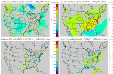
Table 2.Description of the CMAQ model simulations utilized.

CMAQ simulation name CMAQ WRF NEI Photolysis Chemical Simulation period version version version scheme mechanism (all 2011)

CMAQv5.0.2_Base v5.0.2 v3.4 v1 v5.0.2 CB05TULC Annual

CMAQv5.0.2_WRFv3.7 v5.0.2 v3.7 v1 v5.0.2 CB05TUCL January and July

CMAQv5.1_Base_NEIv1 v5.1 v3.7 v1 v5.1 CB05e51 Annual

CMAQv5.1_Base_NEIv2 v5.1 v3.7 v2 v5.1 CB05e51 Annual

CMAQv5.1_Retrophot v5.1 v3.7 v2 v5.0.2 CB05e51 January and July

CMAQv5.1_TUCL v5.1 v3.7 v2 v5.1 CB05e51 January and July

ity System (AQS; 2086 sites; https://www.epa.gov/aqs) for hourly and daily gas and aerosol PM species; the Intera-gency Monitoring of Protected Visual Environments (IM-PROVE; 157 sites; http://vista.cira.colostate.edu/improve/) and Chemical Speciation Network (CSN; 171 sites; https: //www3.epa.gov/ttnamti1/speciepg.html) for daily average (measurements typically made every third or sixth day) to-tal and speciated aerosol PM species; and the Clean Air Status and Trends Network (CASTNET; 82 sites; http:// www.epa.gov/castnet/) for hourly O3 and weekly aerosol

PM species. In addition to these routinely available observa-tions, the DISCOVER-AQ campaign (https://www.nasa.gov/ mission_pages/discover-aq/) during July 2011 provides ad-ditional ground-based gas and aerosol PM measurements, along with unique aloft measurements made by aircraft, ver-tical profilers (e.g., light detection and ranging (lidar) mea-surements), ozonesondes and tethered balloons (not utilized in this analysis, however).

4 Evaluation of major scientific improvements

In this section we evaluate the impact that several of the major scientific improvements in v5.1 have on the opera-tional model performance. Unlike Foley et al. (2010), in which several individual major scientific improvements in CMAQ v4.7 were evaluated incrementally (e.g., each sub-sequent improvement is evaluated against the previous im-provement), here we examine each scientific improvement separately by comparing simulations with the specific im-provement removed (i.e., as it was in v5.0.2) to the base v5.1 simulation (CMAQv5.1_Base_NEIv1) which includes all the updates. While this has the disadvantage of not showing the incremental change in model performance due to each im-provement, it does limit the number of simulations that need to be performed. In addition, it allows for easier examina-tion of the effect of nonlinear increments on total model per-formance, as some updates to the modeling system may be affected by updates to other parts of the model, the effects of which on model performance may not be captured in an incremental testing format. Note that while some attempt is made to broadly identify the processes involved that cause the observed changes in model performance between v5.0.2

and v5.1, it would be too laborious (both to the reader and to the investigators) to comprehensively describe and inves-tigate in depth the processes involved that result in each ob-served difference in model performance described in this tion. Where appropriate, the analyses presented in this sec-tion use the v5.0.2 base simulasec-tion (CMAQv5.0.2_Base) for comparison to the scientific improvement while for other im-provements the v5.1 base simulation is used for comparison. In each case, the simulations being compared are noted. Ta-ble 2 provides a description of the CMAQ model simulations referred to in the following sections.

4.1 WRF and CMAQ meteorological updates

As discussed in Sect. 2.1, there were several significant cor-rections and improvements made to the meteorological cal-culations in both WRF and CMAQ. While the focus of this work is on updates to the CMAQ model, certain options within WRF and CMAQ are linked, and therefore it is neces-sary to discuss the WRF model updates alongside the corre-sponding CMAQ model updates.

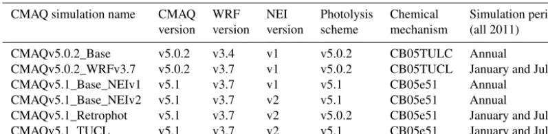
Figure 1 shows the cumulative impact that all the meteoro-logical changes in WRF and CMAQ (i.e., changes to ACM2 and MOL) had on O3and PM2.5in January and July by

com-paring the CMAQv5.0.2_Base simulation to a CMAQv5.0.2 simulation using WRFv3.7 (CMAQv5.0.2_WRFv3.7) which includes the ACM2 and MOL updates. The effect of the changes on O3 in January is mixed, with some areas (e.g.,

Florida, Chicago and the northwest) showing a relatively large (2.5 ppbv) increase in O3, while other areas (e.g., the

southwest and Texas panhandle) show a relatively large de-crease (−2.5 ppbv) in O3. For PM2.5, the differences in

January are generally small and isolated; however, there is a relatively large increase in PM2.5 (>2.5 µg m−3) in the

San Joaquin Valley (SJV) of California due to the updates, which, combined with the decrease in O3there as well,

in-dicates a likely reduction in PBL height and mixing as the cause. There are also some relatively large decreases (1.5– 2.0 µg m−3) in PM2.5in the northeast and around in the Great

Lakes region (i.e., Chicago). Otherwise, most of the remain-ing impacts on PM2.5are relatively small (<1.0 µg m−3).

(9)

Figure 1. Monthly average difference in O3 (ppbv) for (a) January and (b) July and PM2.5 (µg m−3) for (c) January and

(d) July between CMAQv5.0.2 using WRFv3.4 (CMAQv5.0.2_Base) and CMAQv5.0.2 using WRFv3.7 (CMAQv5.0.2_WRFv3.7) (CMAQv5.0.2_WRFv3.7–CMAQv5.0.2_Base). Note that the scales between each plot may vary.

which are considerably larger than the impacts observed in January. The largest increases (4.0–10.0 ppbv) occur in the eastern US, particularly in the southeast. Smaller increases of 2.0–4.0 ppbv occur across much of the US, while in the Gulf of Mexico and the Caribbean O3mixing ratios decrease

roughly 2.0–6.0 ppbv across a large area. The difference in PM2.5in July is similar to that in January, with mostly small,

isolated increases or decreases occurring in the eastern US. The largest increase (2.0–2.5 µg m−3) occurs in the southern Ohio Valley (Kentucky and West Virginia), while the largest decreases (>2.5 µg m−3) occur in Louisiana and Texas (i.e., Houston).

It makes intuitive sense to see summertime O3mixing

ra-tios increasing due to the meteorological changes in WRF and CMAQ, since the net effect of those changes was to in-crease mixing, particularly in the late afternoon and early evening, which in turn decreases the amount of NO titra-tion of O3 that occurs in the model, and ultimately results

in higher O3 mixing ratios on average. Conversely, PM2.5

concentrations would be expected to decrease due to the in-creased mixing in the model, which would effectively de-crease the concentrations of primary emitted pollutants (e.g., EC and organic carbon (OC)), which was observed in ar-eas with the largest emissions (i.e., urban arar-eas). In addition, changes in the oxidant (i.e., OH) concentrations would also potentially affect PM2.5concentrations through increased or

decreased SOA formation (spatial heterogeneity of PM2.5

formation), which results in spatially varying increases and decreases in PM2.5concentrations.

4.2 Aerosol updates

Several new SOA species from anthropogenic VOCs (i.e., AALK1, AALK2, APAH1, APAH2 and APAH3; Table 1) were added to AERO6 in v5.1 that were not present in v5.0.2. Figure 3 shows the difference in the monthly average sum total concentration of these five species for January and July 2011 between the CMAQv5.0.2_Base and CMAQv5.1_Base simulations. Since none of these species were present in v5.0.2, the difference totals in Fig. 2 represent the additional SOA mass that these five species contribute to the total PM2.5

mass in v5.1. For both January and July, the monthly average concentration of these species is small, ranging between 0.0 and 0.1 µg m−3, with the largest concentrations in the east-ern half of the US, particularly in the upper Midwest. How-ever, the concentration of these new species during shorter time periods and smaller, isolated regions would be larger. In addition, the inclusion of these new species is potentially important for health-related studies on the impact of PAHs. Overall, however, these new species represent a small addi-tion to the total PM2.5concentration in the model.

(10)

Figure 2.Monthly average sum total of AALK1, AALK2, APAH1, APAH2 and APAH3 for(a)January and(b)July (upper right) and the monthly average difference is the sum total of AISO1, AISO2, AISO3 and AOLGB for(c)January and(d)July between the aerosol treatments in CMAQ v5.0.2 and v5.1 (v5.1–v5.0.2). All plots are in units of micrograms per cubic meter (µg m−3). Note that the scales between each plot may vary.

of the species containing isoprene SOA (AISO1, AISO2, AISO3 and AOLGB) between v5.1 and v5.0.2. For Jan-uary, the difference in the sum of these species is relatively small, with minimum and maximum values peaking around ±0.5 µg m−3_{, consistent with the fact that isoprene emissions}

are low in winter. For July the difference is always positive (v5.1 higher than v5.0.2) and much larger compared to Jan-uary, with peak differences exceeding 2.5 µg m−3, primarily in the areas with the highest aerosol SO2₄− concentrations (i.e., Ohio Valley). Therefore, the updated IEPOX-SOA for-mation pathways in v5.1 represent a potentially significant contribution to the total PM2.5, particularly during the

sum-mer. Increased isoprene emissions in v5.1 with BEISv3.61 compared to v5.0.2 with BEISv3.14 also contribute to the larger contribution of isoprene SOA in v5.1.

4.3 Cloud model and in-line photolysis updates

Changes in the photolysis and cloud model treatment in v5.1 have potentially significant impacts on the O3and PM2.5

es-timates from the model. Figure 3 shows the difference in O3 and PM2.5for the CMAQv5.1_Base simulation and the

CMAQv5.1_RetroPhot simulation (see Table 2 for simula-tion descripsimula-tion). The CMAQv5.1_RetroPhot simulasimula-tion is the same as the CMAQv5.1_Base simulation except it em-ploys the same (old) photolysis and cloud model treatment as in v5.0.2. For January, O3mixing ratios (Fig. 3a) and PM2.5

concentrations (Fig. 3c) are both higher across the southeast

and portions of California in the v5.1 simulation, indicating that v5.1 has much less photolysis attenuation due to the up-dates in the representation of cloud effects on photolysis.

The impact of the updated photolysis in v5.1 is consid-erably larger in July (when there is more convection) than in January. Peak O3 differences in January were around

2.0 ppbv, whereas in July peak differences of greater than 5.0 ppbv (Fig. 3b) occur over the Great Lakes (where low PBL heights can enhance the impact of changes in O3).

How-ever, in general the difference in O3 mixing ratios is larger

in both magnitude and spatial coverage in July compared to January, indicating that the updated photolysis and cloud model treatment in v5.1 increases O3to a greater extent in

July compared to January, as expected due to increased pho-tolysis rates in the summer compared to winter. Overall, dif-ferences in O3in July range on average from 1.0 to 3.0 ppbv,

with larger differences occurring in the major urban areas (e.g., Atlanta, Charlotte and Los Angeles) and off the coast of the northeast corridor. The change in PM2.5is also larger

(both in magnitude and spatial coverage) in July than Jan-uary (Fig. 3d). The greatest change is primarily confined to the eastern US, resulting in a roughly 0.1 to 0.5 µg m−3 in-crease in PM2.5in v5.1, with the maximum increase located

over the Great Lakes region and areas to the south, the result of increased SOA and gas-phase production of SO2₄−due to greater OH−concentrations in v5.1.

(11)

Figure 3.Difference in the monthly average O3for(a)January and(b)July and PM2.5for(c)January and(d)July between CMAQv5.1_base

and v5.1_RetroPhot (v5.1_Base - v5.1_RetroPhot). O3plots are in units of parts per billion by volume (ppbv) and PM2.5plots are in units

of micrograms per cubic meter (µg m−3). Note that the scales between each plot may vary.

model-predicted cloud albedo at the top of the atmosphere. The predicted cloud albedo from WRFv3.7, CMAQv5.0.2 and CMAQv5.1 were evaluated against cloud albedo from NASA’s Geostationary Operational Environmental Satellite (GOES) Imager product. This evaluation was used to qual-itatively determine whether one CMAQ version better con-siders how clouds affect calculated photolysis rates. The GOES product has a 4 km horizontal resolution and was re-gridded to the 12 km grid structure used in the WRF and CMAQ simulations using the Spatial Allocator utility (https://www.cmascenter.org/sa-tools/). The satellite data are available at 15 min prior to the top of the hour during day-time hours and were matched to model output at the top of the hour. There were 301 h with available satellite data across the domain in July 2011. Figure 4 shows the aver-age cloud albedo (i.e., reflectivity at the top of the atmo-sphere) during these 301 h in July derived from the GOES 35 satellite product (Fig. 4a), and the cloud parameteri-zations within: WRF3.7 (Fig. 4b), CMAQv5.1_RetroPhot (Fig. 4c) and CMAQv5.1_Base_NEIv2 (Fig. 4d). Compar-ison of Fig. 4b and c shows the dramatic differences between the clouds predicted by WRFv3.7 and the predictions from the cloud parameterization in v5.0.2. Most of these large dif-ferences, particularly over land, are now gone in model pre-dictions from the CMAQv5.1_Base simulation, which uses resolved clouds from WRF and subgrid clouds from the con-vective cloud model within CMAQ (compare Fig. 4b to d).

Two notable issues remain with the v5.1 modeled cloud parametrization. The photolysis cloud parameterization in v5.1 produces more clouds over water compared to the WRF parameterization, which is itself biased high for some parts of the Atlantic Ocean compared to GOES. This issue will be addressed by science updates planned for the CMAQ system, and evaluation results are expected to improve in the next CMAQ release. A more significant issue, from an air quality perspective, is the underprediction of clouds over much of the eastern and west-central US in the WRF-predicted clouds, which is now directly passed along to CMAQ. This misclas-sification of modeled clear sky conditions can contribute to an overprediction of O3 in these regions. Resolving this

is-sue will require changes to the WRF cloud parameterization. Future research will also include changing the subgrid cloud treatment currently used in the CMAQ system to be consis-tent with the subgrid parameterization used in WRF. Sec-tion S1 in the Supplement provides a table with addiSec-tional evaluation metrics of the modeled clouds over oceans vs. over land and also describes how cloud albedo was calcu-lated for the three model simulations.

4.4 Atmospheric chemistry updates

(12)

31

(a) GOES (b) WRFv3.7

(c) CMAQv5.1_RetroPhot (d) CMAQv5.1_Base

Figure 4. The average cloud albedo during daytime hours in July 2011 derived from (a) the GOES satellite product (b) WRF3.7 (c) CMAQv5.1 with photolysis/cloud model treatment from v5.0.2 and WRF3.7 inputs (CMAQv5.1_RetroPhot) (d) CMAQv5.1 using WRF3.7 inputs (CMAQv5.1_Base).

Figure 4. The average cloud albedo during daytime hours in July 2011 with available satellite data (n=301 h total) derived from(a)

the GOES satellite product, (b) WRF3.7,(c) CMAQv5.1 with photolysis and cloud model treatment from v5.0.2 and WRF3.7 inputs (CMAQv5.1_RetroPhot), and(d)CMAQv5.1 using WRF3.7 inputs (CMAQv5.1_Base_NEIv2).

order to assess the overall impact that the combined chem-istry changes have on the model results, model comparisons are conducted using the CMAQv5.1_Base simulation, which employs the CB05e51 chemical mechanism (the v5.1 default chemical mechanism) and the CMAQv5.1_TUCL simulation (see Table 2 for description). The CMAQv5.1_TUCL sim-ulation is the same as the CMAQv5.1_Base simsim-ulation ex-cept that it employs the CB05TUCL chemical mechanism (Whitten et al., 2010; Sarwar et al., 2012), the default mech-anism in v5.0.2. Note that the aerosol updates discussed in Sect. 4.2 were incorporated into the CB05e51 chemical mechanism (in the past that portion of the aerosol chem-istry was separate from the gas-phase chemical mechanism). As such, differences between the CMAQv5.1_TUCL and CMAQv5.1_Base_NEIv2 simulations include impacts from those changes (i.e., Fig. 2). In order to isolate primarily just the effect on PM2.5from the atmospheric chemistry changes,

the organic matter (AOMIJ; see Sect. 2 and 3 for species def-inition descriptions) mass has been removed from the com-parisons of total PM2.5mass discussed below.

Figure 5 shows the difference in monthly aver-age O3 and PM2.5 for January and July between the

CMAQv5.1_Base_NEIv2 and CMAQv5.1_TUCL sim-ulations. For January, O3 mixing ratios are higher

in the simulation using the CB05e51 mechanism (CMAQv5.1_Base_NEIv2 simulation); however, the overall

impact of CB05e51 on O3 is generally small (∼2–4 %),

with maximum differences of only approximately 1.0 ppbv (∼6 %), primarily along the southern coastal areas of the US. PM2.5is also higher in January in the simulation using

the CB05e51 mechanism (CMAQv5.1_Base_NEIv2 simula-tion), with the largest changes in PM2.5 of 0.2–0.4 µg m−3

(∼2–6 %) primarily occurring in the eastern US and greater than 1.0 µg m−3(∼6–8 %) in the SJV of California.

For July, O3 mixing ratios are higher across most areas

in the CMAQv5.1_Base_NEIv2 simulation, primarily across northern portions of the US, the Great Lakes region and in California (i.e., Los Angeles and the SJV). Most increases in O3in the CMAQv5.1_Base simulation range between 0.6

and 1.2 ppbv (∼2–4 %); however, larger increases of over 3.0 ppbv (∼4–8 %) occur in southern California and over Lake Michigan (likely influenced in part by low PBL heights over the lake). A small area of lower O3mixing ratios occurs

off the eastern coast of the US. For July, the difference in PM2.5due to the CB05e51 chemical mechanism is relatively

small, with differences in concentrations generally ranging from±0.50 µg m−3(∼2–4 %) across the eastern US.

5 Evaluation of CMAQv5.1

(13)

sim-Figure 5.Difference in the monthly average O3for(a)January and(b)July and PM2.5(with organic matter mass removed) for(c)January

and(d)July between CMAQv5.1_Base_NEIv2 and v5.1_TUCL (CMAQv5.1_Base_NEIv2–CMAQv5.1_TUCL). O₃plots are in units of parts per billion by volume (ppbv) and PM2.5plots are in units of micrograms per cubic meter (µg m−3). Note that the scales for each plot

can vary.

ulations by initially comparing the simulations to each other (model to model) and then evaluating them against a wide va-riety of available air quality measurements (see Sect. 3). Sev-eral common measurements of statistical performance are used, namely mean bias (MB), mean error (ME), root mean square error (RMSE) and Pearson correlation. Note that representativeness (incommensurability) issues are present whenever gridded values from a deterministic model such as CMAQ are compared to observed data at a particular point in time and space, as deterministic models calculate the aver-age outcome over a grid for a certain set of given conditions, while the stochastic component (e.g., subgrid variations) em-bedded within the observations cannot be accounted for in the model (Swall and Foley, 2009). These issues are some-what mitigated for networks that observe for longer dura-tions, for example the CSN and IMPROVE networks, which are daily averages, and the CASTNET observations, which are weekly averages. The longer temporal averaging helps reduce the impact of stochastic processes, which can have a large impact on shorter (e.g., hourly) periods of observation (Appel et al., 2008).

There are a couple of important differences to keep in mind between the comparison of the CMAQv5.0.2_Base and CMAQv5.1_Base_NEIv1 simulations beyond the obvi-ous changes to the model process representations discussed in the previous sections. First, the simulations use different

versions of WRF (as discussed in Sects. 2.2 and 4.1). This was intentional, as it was determined that the changes made from WRFv3.4 (used in the CMAQv5.0.2_Base simulation) to WRFv3.7 (used in the CMAQv5.1_Base_NEIv1 simula-tion) and subsequent required changes made to the CMAQ code represent a change to the overall WRF–CMAQ mod-eling system and therefore should be evaluated together. It should also be noted that the windblown dust treatment was employed in the CMAQv5.0.2_Base simulation but not in the CMAQv5.1_Base_NEIv1 simulation. This was due to issues with the implementation of the updated windblown dust treatment in v5.1 that were not discovered until after the model was released and the CMAQv5.0.2_Base simula-tion was completed. However, the contribusimula-tion of windblown dust to total PM2.5in v5.0.2 tends to be small and episodic

and therefore should not constitute a significant impact to the performance differences between v5.0.2 and v5.1, espe-cially for the monthly averages generally shown here. How-ever, we make an attempt to note when and where the impact from windblown dust is apparent. For reference, the v5.0.2-simulated seasonal average values of PM2.5 and maximum

daily 8 h average (MDA8) O3 are provided in Figs. S1 and

(14)

Figure 6.Difference in the seasonal average PM2.5for(a)winter (DJF),(b)spring (MAM),(c)summer (JJA) and(d)fall (SON) between

CMAQv5.0.2_Base and CMAQv5.1_Base_NEIv1 (CMAQv5.1_Base_NEIv1–CMAQv5.0.2_Base). All plots are in units of micrograms per cubic meter (µg m−3).

5.1 PM2.5

Figure 6 shows the seasonal average difference in model-simulated PM2.5 between v5.0.2 and v5.1

(CMAQv5.1_Base_NEIv1–CMAQv5.0.2_Base), with cool colors indicating a decrease in PM2.5 in v5.1 (vs.

v5.0.2) and warm colors indicating an increase in PM2.5.

Figure 7 shows the seasonal MB for PM2.5 for the

CMAQv5.1_Base_NEIv1 simulation, while Figure 8 shows the change in the absolute value of the sea-sonal MB in PM2.5 between the CMAQv5.0.2_Base and

CMAQv5.1_Base_NEIv1 simulations. Cool colors indicate smaller PM2.5 MB in the CMAQv5.1_Base_NEIv1

simu-lation (vs. the CMAQv5.0.2_Base simusimu-lation), while warm colors indicate larger MB in the CMAQv5.1_Base_NEIv1 simulation.

During winter, v5.1 simulates lower PM2.5concentrations

in the eastern US and portions of central Canada compared to v5.0.2, and higher PM2.5concentrations in the SJV (Fig. 6).

PM2.5is largely overestimated in the eastern US and

under-estimated in the western US (the exception being portions of the northwest) in the winter in the CMAQv5.1_Base_NEIv1 simulation (Fig. 7a). The change in MB between v5.0.2 and v5.1 is negative (reduced MB in v5.1) across the majority of the sites, with relatively large reductions (3–5 µg m−3) in MB in the northeast, upper Midwest (i.e., Great Lakes re-gion) and the SJV (Fig. 8a). Figure S3 presents a histogram

of the change in PM2.5 MB using the same data and color

scale as in Fig. 8. It is clear from the histogram that there is a large percentage (72.3 %) of sites where the MB de-creases in the CMAQv5.1_Base_NEIv1 simulation in the winter (Fig. S3a), demonstrating a widespread improvement in the PM2.5performance for v5.1 vs. v5.0.2.

The diurnal profile of PM2.5for winter (Fig. 9a) indicates

a relatively large decrease in MB throughout most of the day with v5.1 vs. v5.0.2, particularly during the overnight, morning and late afternoon hours. A similar improvement is seen in the RMSE, and the correlation also improves for all hours (Fig. S5). Figure 10 shows seasonal and regional stacked bar plots of PM2.5composition (SO42−, NO−3, NH

+

4,

(15)

Ari-33

Figure 7: Seasonal average PM2.5 mean bias (µgm-3) at IMPROVE (circles), CSN (triangles), AQS Hourly (squares) and AQS Daily (diamonds) sites for

a) winter (DJF) b) spring (MAM) c) summer (JJA) and d) fall (SON) for the CMAQ v5.1_Base simulation.

(a) Winter PM2.5 mean bias (v5.1 - Obs) (b) Spring PM2.5 mean bias (v5.1 - Obs)

(c) Summer PM2.5 mean bias (v5.1 - Obs) (d) Fall PM2.5 mean bias (v5.1 - Obs)

Figure 7.Seasonal average PM2.5mean bias (µg m−3) at IMPROVE (circles), CSN (triangles), AQS Hourly (squares) and AQS Daily

(diamonds) sites for(a)winter (DJF),(b)spring (MAM),(c)summer (JJA) and(d)fall (SON) for the CMAQv5.1_Base simulation.

Figure 8: Difference in the absolute value of seasonal average PM2.5 mean bias for a) winter (DJF) b) spring (MAM) c) summer (JJA) and d) fall (SON)

between CMAQ v5.0.2_Base and v5.1_Base (CMAQv5.1_Base – CMAQv5.0.2_Base). All plots are in units of µgm-3_{. Cool colors indicate a reduction in}

PM2.5 mean bias in v5.1 while warm color indicate an increase in PM2.5 mean bias v5.1.

(a) Winter PM2.5|MB|;(|v5.1 –Obs| –|v5.0.2 –Obs|) (b) Spring PM2.5|MB|; (|v5.1 –Obs| –|v5.0.2 –Obs|)

(c) Summer PM2.5|MB|;(|v5.1 –Obs| –|v5.0.2 –Obs|)(d) Fall PM2.5 |MB|;(|v5.1 –Obs| –|v5.0.2 –Obs|)

Figure 8.Difference in the absolute value of seasonal average PM2.5mean bias for(a)winter (DJF),(b)spring (MAM),(c)summer (JJA)

and (d)fall (SON) between CMAQ v5.0.2_Base and v5.1_Base_NEIv1 (CMAQv5.1_Base_NEIv1–CMAQv5.0.2_Base). All plots are in units of micrograms per cubic meter (µg m−3). Cool colors indicate a reduction in PM2.5mean bias in v5.1, while warm colors indicate an

increase in PM2.5mean bias v5.1.

(16)

Figure 9. Diurnal time series of seasonal PM2.5 (µg m−3) for AQS observations (gray), CMAQv5.0.2_Base simulation (blue) and

CMAQv5.1_Base_NEIv1 simulation (red) for(a)winter,(b)spring,(c)summer and(d)fall.

zona, Nevada and New Mexico). These regions are derived from principle component analysis to group states with simi-lar PM2.5source regions together. For winter, the total PM2.5

high bias is reduced across all five regions, with most of the improvement coming from reductions in OC, non-carbon or-ganic matter (NCOM; see Sect. 2 or 3 for definition) and Other, indicating that improvements in the representation of mixing under stable conditions helped in reducing the high bias. Still, a large bias remains for OC, which may be due in

part to an overestimation of the residential wood combustion in the NEI.

For spring, the changes in PM2.5are much more isolated

than in winter (Fig. 6b), with the largest decreases occurring around Montreal (Canada) and portions of the Midwest and desert southwest (lack of windblown dust in v5.1 contributes to the decrease in the desert southwest). The MB for PM2.5in

(17)

underes-Figure 10.Regional and seasonal stacked bar plots of PM2.5composition at the CSN sites (left), CMAQv5.0.2_Base simulation (middle)

and CMAQv5.1_Base_NEIv1 simulation (right). In order from top to bottom are(a)winter,(b)spring,(c)summer and(d)fall seasons and left to right the northeast, Great Lakes, Atlantic, south and west regions. The individual PM2.5components (in order from bottom to top)

are SO2₄−(yellow), NO−₃ (red), NH+₄ (orange), EC (black), OC (light gray), soil (brown), NaCl (green), NCOM (pink), other (white), blank adjustment (dark gray) and H2O/FRM adjustment (blue).

timations in Texas and larger overestimations in the north-east, Great Lakes and northwest (Fig. 7b). As expected with the relatively small change in modeled PM2.5concentrations

with v5.1 in the spring (Fig. 6b), the difference in MB be-tween v5.0.2 and v5.1 is relatively small, with most differ-ences in MB less than±1.0 µg m−3(Fig. 8b). Some slightly larger decreases in MB occur in the northeast and northwest, while some larger increases in MB occur in the Midwest and Texas. A little more than half (53.0 %) of the sites report an improvement in MB (Fig. S3b). The diurnal profile of PM2.5

for spring shows a consistent underestimation of PM2.5

throughout most of the day in the v5.0.2 simulation, which becomes larger in the CMAQv5.1_Base_NEIv1 simulation, with an overall decrease in PM2.5 in the spring (Fig. 9b).

However, the RMSE is lower during the overnight, morning

and afternoon hours in the CMAQv5.1_Base_NEIv1 simula-tion, and the correlation improves throughout most of the day as well (Fig. S5). Total PM2.5MB improves in three of the

five regions shown in Fig. 10, with most of the improvement coming from lower concentrations of OC and NCOM.

In the summer, PM2.5 is considerably higher

(>5.0 µg m−3) across a large portion of the eastern US in the CMAQv5.1_Base_NEIv1 simulation, particularly in Mississippi, Alabama, Georgia and portions of the Ohio Valley (Fig. 6c). The increase in PM2.5 is primarily due to

the updates to the IEPOX-SOA chemistry in v5.1 (Fig. 2), updates to BVOC emissions in BEISv3.61 (approximately 1.0 µg m−3_{increase PM}

2.5in the southwestern US), and the

(18)

36

Figure 11: Difference in the monthly average hourly O3 (ppbv) for winter (DJF; top left), spring (MAM; top right), summer (JJA; bottom left) and fall

(SON; bottom right) between CMAQ v5.0.2_Base and v5.1_Base (CMAQv5.1_Base – CMAQv5.0.2_Base). Note that the scales for each plot can vary.

(a) Winter O3 mean difference (v5.1 – v5.0.2) (b) Spring O3 difference (v5.1 – v5.0.2)

(c) Summer O3 difference (v5.1 – v5.0.2) (d) Fall O3 difference (v5.1 – v5.0.2)

Figure 11.Difference in the monthly average hourly O3(ppbv) for winter (DJF; top left), spring (MAM; top right), summer (JJA; bottom

left) and fall (SON; bottom right) between CMAQ v5.0.2_Base and v5.1_Base_NEIv1 (CMAQv5.1_Base_NEIv1–CMAQv5.0.2_Base). Note that the scales between each plot may vary.

mechanism (Fig. 5) and updates to the clouds/photolysis (Fig. 3). Despite the increase in PM2.5 with v5.1, PM2.5

still remains largely underestimated in the summer, with the largest underestimations in the southeastern US, Texas and California (Fig. 7c). However, the result of the widespread increase in PM2.5 with v5.1 is a similar large, widespread

reduction in the MB across the eastern US, particularly in the southeast and the Ohio Valley, where reductions in MB range from 3.0 to 5.0 µg m−3 (Fig. 8c). Smaller increases in the MB (typically less than 2.0 µg m−3) occur in Florida and isolated areas in the western US. Of all the sites, 69.8 % report an improvement in MB, with a number of sites show-ing reductions in MB greater than 5.0 µg m−3 (Fig. S3c). PM2.5 is underestimated throughout the day in both the

v5.0.2 and v5.1 simulations (Fig. 9c) in summer, with the underestimation improving slightly with v5.1, particularly during the afternoon and overnight hours. RMSE improves during the daytime hours with v5.1, while correlation is considerably higher with v5.1 than v5.0.2 throughout the entire day (Fig. S6). Total PM2.5 is underestimated in the

CMAQv5.0.2_Base simulation in four of the five regions (the west region being the exception), which improves in the CMAQv5.1_Base_NEIv1 simulation (Fig. 10). The overestimation in the west region with v5.0.2 also improves with v5.1. Small increases in SO2₄− and NH+₄ and larger increases in OC and NCOM contribute to the improvement.

For the fall, the difference in PM2.5 between v5.0.2 and

v5.1 is again small, with the largest increases occurring in isolated portions of the eastern US and California, and the largest decreases occurring in Montreal and isolated areas in the western US (Fig. 6d). The MB pattern in the fall (Fig. 7d) is similar to the one in the spring as well (Fig. 7b), with rela-tively small MBs in the eastern US (±2.0 µg m−3) and larger MBs along the west coast (underestimated in California and overestimated in the northwest). As expected, the change in the MB between v5.0.2 and v5.1 is also relatively small in the fall, with the majority of the sites reporting a change in MB of less than±2.0 µg m−3(Fig. 8d), and 68.1 % of the sites reporting a reduction in MB (Fig. S3d). The average diurnal profile of PM2.5in the fall (Fig. 9d) is similar to the spring,

with improved MB with v5.1 during the overnight, morn-ing and late afternoon or evenmorn-ing hours and reduced RMSE and improved correlation throughout the entire day (Fig. S8). Total PM2.5 is overestimated in all five regions in the fall

(Fig. 10), but improves with v5.1 in all of those regions (al-beit only very slightly for the south region), with decreases in EC and OC responsible for most of the improvement.

5.2 Ozone

For the winter, O3 widely decreases in the

(19)

37

Figure 12: Seasonal average hourly O3 mean bias at AQS sites for a) winter (DJF) b) spring (MAM) c) summer (JJA) and d) fall (SON) for the CMAQ

v5.1_Base simulation. All plots are in units of ppbV.

(a) Winter O3 mean bias (v5.1 - Obs) (b) Spring O3 mean bias (v5.1 - Obs)

(c) Summer O3 mean bias (v5.1 - Obs) (d) Fall O3 mean bias (v5.1 - Obs)

Figure 12.Seasonal average hourly O3(ppbv) mean bias at AQS sites for(a)winter (DJF),(b)spring (MAM),(c)summer (JJA) and(d)fall

(SON) for the CMAQv5.1_Base_NEIv1 simulation.

Figure 13: Difference in the absolute value of monthly average O3 mean bias for a) winter (DJF) b) spring (MAM) c) summer (JJA) and d) fall (SON)

between CMAQ v5.0.2_Base and v5.1_Base (CMAQv5.1_Base – CMAQv5.0.2_Base). All plots are in units of ppbV. Cool colors indicate a reduction in O3 mean bias in v5.1 while warm color indicate an increase in O3 mean bias v5.1.

(a) Winter O3 |MB|; (|v5.1 – Obs| – |v5.0.2 – Obs|) ( Spring Ob) 3 |MB|; (|v5.1 – Obs| – |v5.0.2 – Obs|)

(c) Summer O3 |MB|; (|v5.1 – Obs| – |v5.0.2 – Obs|) (d) Fall O3 |MB|; (|v5.1 – Obs| – |v5.0.2 – Obs|)

Figure 13.Difference in the absolute value of monthly average O3(ppbv) mean bias for(a)winter (DJF),(b)spring (MAM),(c)summer

(JJA) and(d)fall (SON) between CMAQ v5.0.2_Base and v5.1_Base_NEIv1 (CMAQv5.1_Base_NEIv1–CMAQv5.0.2_Base). Cool colors indicate a reduction in O₃mean bias in v5.1, while warm colors indicate an increase in O₃mean bias v5.1.

(20)

Figure 14. Diurnal time series of seasonal O3 (ppbv) for AQS observations (gray), CMAQv5.0.2_Base simulation (blue) and

CMAQv5.1_Base_NEIv1 simulation (red) for(a)winter,(b)spring,(c)summer and(d)fall.

with the seasonal average decreases ranging between 1.0 and 3.0 ppbv, and several areas where decreases exceed 3.0 ppbv, primarily over the oceans (Fig. 11a). In the eastern US, the change in O3is relatively small and isolated. Ozone

is underestimated at most sites across the northern portion of the US, with the largest underestimations occurring in Colorado, Wyoming and Utah. Despite the decreases in O3

with v5.1, O3is still overestimated in the southwestern US

and California (Fig. 12a). There is a widespread reduction

in the O3MB in California and increased MB in the upper

Midwest with v5.1, while across the rest of the domain the change in MB is relatively small (Fig. 13a). The majority of the change in O3 falls between ±5.0 ppbv, with 56.5 %

reporting a reduction in MB (Fig. S8a). The average diurnal profile of O3 in the winter (Fig. 14a) shows slightly lower

(21)

Figure 15. Diurnal time series of seasonal NOx (ppbv) for AQS observations (gray), CMAQv5.0.2_Base simulation (blue) and CMAQv5.1_Base_NEIv1 simulation (red) for(a)winter,(b)spring,(c)summer and(d)fall.

and RMSE, and higher correlation throughout the day with v5.1 vs. v5.0.2 (Fig. S9). The NOx diurnal profile also

gen-erally improves throughout the day in winter (Fig. 15a), with decreased MB and RMSE in the afternoon or early evening and increased correlation throughout the day (Fig. S11).

The pattern of change in O3 between v5.0.2 and v5.1 in

spring is similar to winter, with lower O3mixing ratios in the

western US and higher mixing ratios in the eastern US in v5.1 compared to v5.0.2 (Fig. 11b). Decreases in O3mixing ratios

in the western US in v5.1 range from roughly 1.0 to 3.0 ppbv (similar to winter), while in the eastern US the increases gen-erally range from 1.0 to 2.0 ppbv, with isolated areas of larger increases. The MB of O3 for the v5.1 simulation primarily

ranges from slightly overestimated to slightly underestimated across most the sites, with larger overestimations along the

Gulf Coast and larger underestimations in the western US (Fig. 12b). The change in MB between v5.0.2 and v5.1 shows mixed results (Fig. 13b), with slight increases and decreases across much of the eastern US and a relatively large increase in MB in the Midwest (i.e., Colorado and Wyoming). The MB mostly improved across the Gulf Coast and in California due to reduced O3mixing ratios from the new marine

halo-gen chemistry and enhanced O3deposition to ocean surfaces.

Half of the sites reported a reduction in MB (Fig. S8b) with v5.1. The diurnal profile of O3for spring (Fig. 14b) shows