Implementation and validation of the
extended Hill‑type muscle model with robust
routing capabilities in LS‑DYNA for active
human body models
Christian Kleinbach
1*†, Oleksandr Martynenko
2†, Janik Promies
1, Daniel F. B. Haeufle
3, Jörg Fehr
1and Syn Schmitt
2Background
It is hard to imagine that the development of modern vehicles can be done without wide utilization of computer aided engineering (CAE), including state-of-the-art numerical simulations software. These tools not only offer opportunities to the car manufacturers
Abstract
Background: In the state of the art finite element AHBMs for car crash analysis in the LS-DYNA software material named *MAT_MUSCLE (*MAT_156) is used for active mus-cles modeling. It has three elements in parallel configuration, which has several major drawbacks: restraint approximation of the physical reality, complicated parameteriza-tion and absence of the integrated activaparameteriza-tion dynamics. This study presents implemen-tation of the extended four element Hill-type muscle model with serial damping and eccentric force–velocity relation including Ca2+ dependent activation dynamics and internal method for physiological muscle routing.
Results: Proposed model was implemented into the general-purpose finite element (FE) simulation software LSDYNA as a user material for truss elements. This material model is verified and validated with three different sets of mammalian experimen-tal data, taken from the literature. It is compared to the *MAT_MUSCLE (*MAT_156) Hill-type muscle model already existing in LS-DYNA, which is currently used in finite element human body models (HBMs). An application example with an arm model extracted from the FE ViVA OpenHBM is given, taking into account physiological mus-cle paths.
Conclusion: The simulation results show better material model accuracy, calcula-tion robustness and improved muscle routing capability compared to *MAT_156. The FORTRAN source code for the user material subroutine dyn21.f and the muscle parameters for all simulations, conducted in the study, are given at https://zenodo. org/record/826209 under an open source license. This enables a quick application of the proposed material model in LS-DYNA, especially in active human body models (AHBMs) for applications in automotive safety.
Keywords: Hill-type muscle model, LS-DYNA, Muscle routing, Human body model, Finite element analysis, Biomechanics
Open Access
© The Author(s) 2017. This article is distributed under the terms of the Creative Commons Attribution 4.0 International License (http://creativecommons.org/licenses/by/4.0/), which permits unrestricted use, distribution, and reproduction in any medium, provided you give appropriate credit to the original author(s) and the source, provide a link to the Creative Commons license, and indicate if changes were made. The Creative Commons Public Domain Dedication waiver (http://creativecommons.org/publicdo-main/zero/1.0/) applies to the data made available in this article, unless otherwise stated.
SOFTWARE
*Correspondence: christian.kleinbach@itm. uni-stuttgart.de †Christian Kleinbach and Oleksandr Martynenko contributed equally to this work
for saving time and costs during the design phase, but also to model and predict future product lifecycle. One of the most demanding and regulated domains is vehicle safety and therefore crash simulations. For more than a quarter of a century, complete vehicles are modelled virtually as finite element models with all significant details, including mate-rial and geometrical properties. The same approach was then applied to the human body, and in the last decade several detailed finite element human body models (HBMs) were presented [1–3]. Joint simulations with a combined application of car and human body models allow for prediction of in-crash behaviour and possible injuries for occupants or pedestrians with a sufficient accuracy throughout all stages in development, replacing expensive crash tests using car prototypes and Anthropomorphic Test Devices (ATDs).
These so-called virtual testing methods will gain importance in the future, as the cur-rent trends of active safety systems and autonomous vehicles become available on the market. Active safety systems, in contrast to traditional passive safety systems, react preventively prior to a crash to avoid or mitigate a possible impact. This requires active HBMs (AHBMs) that are able to reproduce human behaviour in normal driving situ-ations, as well as the behaviour in the in-crash phase. The same requirements exist for the second trend of autonomous vehicles, where generic driving or sitting positions no longer exist, but where occupants can move freely. From these requirements, three chal-lenges for AHBM modelling arise. The first being the implementation of active muscles as mathematical models of the muscle-tendon complex (MTC) including the activation dynamics, which will be addressed in the contribution. The second challenge is to model biologically relevant neural controllers to enable accurate forward dynamics (FD) sim-ulations of human reactions and voluntary motion in all kind of traffic scenarios. The third challenge is the choice of parameters for AHBMs, as only a correct representation of both the passive components and active components will result in an accurate rep-resentation of a living human. Most current HBMs have a passive stiffness which is too high, see e.g. [4, 5]. On the one hand, this is to compensate for the active components still missing. On the other hand, this is because the source for the parameters are almost exclusively post mortem human subjects, where tissue modulus and no-load strain differ from living tissue depending on the postmortem time and post-mortem rigor [6].
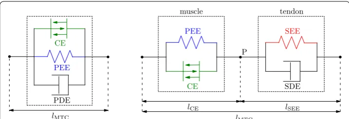
In the state of the art finite element AHBMs [7, 8] for car crash analysis the LS-DYNA material named *MAT_MUSCLE (*MAT_156) is used for modeling active muscles. This
PDE PEE
CE
lMTC
SDE PEE
CE
lMTC
lCE lSEE
SEE
muscle tendon
P
material is an advanced version of the previous model *MAT_SPRING_MUSCLE [9] for discrete elements, that is no longer being supported. *MAT_156 represents a Hill-type muscle model which consists of three parallel elements: contractile element (CE), parallel elastic element (PEE) and a parallel damping element (PDE), see also Fig. 1a. The imple-mentation was done by Dr. J. A. Weiss based on prior studies and reviews on different Hill-type model element configurations by [10–12]. The implemented configuration was chosen due to its simplicity, ease of parameters derivation from the experiments and computational efficiency. However, in the publication [12] it was pointed out, that an element configura-tion with better approximaconfigura-tion of the physical reality should be used in simulaconfigura-tions if pos-sible. Such an extended Hill-type muscle model should have a clear separation between muscle fibres and tendon structures. For a correct representation of the MTC dynamics an additional internal degree of freedom is required to decouple active muscle fibre and elas-tic tendon dynamics. Subsequent studies investigating the role of the serial elaselas-tic element have shown, that such simplifications and assumptions can lead to instabilities produced by force-velocity or force-length relation formulations [13], incorrect energy storage and release in the interaction with the environment [14, 15], unrealistic high-frequency oscil-lations [16] and differences in muscle force magnitude [17]. All these effects, mentioned in publications above, directly influence the explicit integration scheme used in LS-DYNA thus impacting speed, accuracy and robustness of simulations with AHBMs.
Usually, muscles and tendons wrap around bones or joints in both steady state condi-tions and while performing movements, consequently a physiological muscle path rep-resentation (muscle routing) is essential for FD simulations [18, 19]. Slight changes in the muscle line of action will lead to inaccurate muscle forces and resulting moments due to incorrect lever arms and muscle length. To model physiological muscle paths in finite element HBMs different muscle routing methods can be used. Fixed lever arms or the via-point method [20, 21] are the most simple options and the usage of contact detection [22] would be the most sophisticated method. According to [23] a via-point method should be preferred for *MAT_156 using the *ELEMENT_BEAM_PULLEY key-word in LS-DYNA. However, it is unclear if this method is applicable, as there exist so far no successful implementation of this method in AHBMs to the authors knowledge.
Additional disadvantages result from the way parameters are set for *MAT_156 in LS-DYNA. For a number of parameters predefined curves are required, e.g. muscle activation level vs. time or stress vs. the stretch ratio. These curves need to be defined beforehand or might be calculated during the runtime through the *DEFINE_CURVE_ FUNCTION keyword and PIDCTL [24] options. This approach is limited, cumbersome and error prone. Instead, muscle parameters and constants found in anatomico-phys-iological literature should be used directly. Also, some disadvantages exist for muscle activation dynamics. Predefined muscle activation level vs. time curves cannot represent the activation dynamics correctly and to model the dynamics more precisely the activa-tion level has to depend on the muscle length. The complete activaactiva-tion dynamics can be included efficiently in the material model for the muscle itself.
The complete description of the model, its implementation, verification and validation are given in the next sections.
Methods
In this section the complete model, its implementation in LS-DYNA, and the verifica-tion and validaverifica-tion set-up are described.
Muscle model
One of today’s most popular and widely used macroscopic muscle model was proposed by Hill in 1938 [26] on the basis of experiments with frog muscles. The most important feature is a direct relation between muscle force and contraction velocity. Furthermore the model is also referred to as a first order muscle model, which means, that the muscle elements have neither mass nor inertia, and only an axial force is applied on the skeletal model between origin and insertion point of the muscle. During the past years some dis-advantages of the original Hill model were found and there have been many publications with the aim of further developing and improving this model.
In the publication of Haeufle et al. [25], a modified Hill-type muscle model was proposed with improved serial damping and eccentric force-velocity relation. This model consists of four simple mechanical elements: an active contractile element (CE), which is controlled by the activation level q; parallel (PEE) and serial (SEE) nonlinear spring elements and a serial damping element (SDE). The model’s structure was based on a previous study by Günther et al. [16] which determined, that the model with a force-dependent SDE pro-vides the best results in a comparison with constant parallel, constant serial, and force-dependent parallel damping elements. The structure of the MTC of the Haeufle model is shown in Fig. 1b, with two clearly separated parts modeling the active muscle fibres (CE + PEE) and the passive tendon and aponeurosis structures (SEE + SDE). The main equations of the muscle model are presented in the following. They were taken from [16, 19, 25, 27], where more detailed explanations can be found if needed. Furthermore, a comprehensive study on the influence of individual parts and their model formulation is given in [28].
As shown in Fig. 1b the muscle model features an internal degree of freedom which is described by lCE . The lengths of the passive elements are equal to
Then the total MTC length is
The force equilibrium at point P between the muscle fibre and the tendon part is described in [16] as:
Contractile element (CE)
The contractile element represents the active fibre bundles of the MTC. The force of the contractile element FCE is therefore dependent on the muscle activity q, the contraction
(1) lPEE=lCE
(2)
andlSDE=lSEE.
(3)
lMTC=lCE+lSEE.
(4)
velocity ˙lCE as well as the length-dependent isometric force Fisom(lCE). It is expressed by
the equation
The factors Arel and Brel are so-called normalized Hill parameters, where Arel is nor-malized with the maximum isometric force Fmax and Brel with the optimal fibre length
lCE,opt [16, p. 64]. The subscript ‘rel’, for relative, indicates the normalization. The opti-mal muscle fibre length at which the isometric force reaches the maximum value is
lCE,opt . The isometric force Fisom depends on the length of the contractile element and is calculated as follows:
This equation represents the bell-shaped force-length relationship of the CE element. The width of the normalized bell curve Wlimb and the exponent νCE,limb may be chosen differently for the ascending and descending limb of the force-length curve.
When calculating the Hill parameters, it is distinguished between an eccentric ˙l CE>0
(lengthening fibres) and a concentric case ˙l
CE≤0 (shortening fibres). Please note, that in
physiological muscle experiments, where shortening work of muscle fibres is examined, the sign convetion for the contraction velocity is usually the opposite (shortening fibres have a positive velocity) to ensure that the work of shortening muscles is positive. In the concentric case, the Hill parameters are:
The auxiliary variables for the calculation of the Hill parameters are divided into length- and activation-dependent components. The length-dependent parameters are defined as:
and the activation-dependent as:
The equations in the eccentric case can be derived from Eq. (5) as mentioned in [25] and thus they are formulated as:
(5)
FCE(lCE,˙lCE,q)=Fmax
qFisom+Arel
1− ˙lCE
BrellCE,opt −Arel
.
(6)
Fisom(lCE)=exp
− � � � � � �
lCE
lCE,opt −1
�Wlimb
� � � � � �
νCE,limb
.
(7) Arel(lCE,q)=Arel,0·LArel(lCE)·QArel(q),
(8) Brel(lCE,q)=Brel,0·LBrel(lCE)·QBrel(q).
(9)
LArel=
1, lCE<lCE,opt
Fisom, lCE≥lCE,opt ,LBrel(lCE)=1
(10)
QArel(q)= 1
4(1+3q),
(11)
QBrel(q)= 1
and
Parallel elastic element (PEE)
The PEE represents passive properties of the muscle fiber and the collagenous connec-tive tissue surrounding the muscle belly. As soon as the length of the contractile element exceeds the resting length of the parallel elastic element lPEE,0, it also contributes to the force developed by the MTC. Mathematically this is expressed as:
The spring stiffness KPEE is influenced by the optimal fibre length, the width of the bell
curve and the maximum isometric force. It is calculated by:
The resting length is defined as lPEE,0=LPEE,0·lCE,opt, hence LPEE,0 is the resting length normalized by lCE,opt , Wdesc is width of Fisom(lCE) on a descending limb.
Serial elastic element (SEE)
Since structures similar to muscle tissue are also present in the tendon, their elastic properties are similar. The serial elastic element has a nonlinear or linear spring behav-iour depending on the deflection lSEE. When lSEE<lSEE,0 the tendon is relaxed and does not generate any force. In the range of lSEE,0<lSEE<lSEE,nll it has a nonlinear character-istic, and a linear characteristic for lSEE≥lSEE,nll:
The length lSEE,nll of the SEE at the transition from nonlinear to linear characteristic, the exponent νSEE, and the nonlinear and linear stiffness factors KSEE,nl and KSEE,l are defined by the following formulas:
The complete description of these independent parameters can be found in [16, Fig. 4, p. 69].
(12)
Arel,e= −Fe·q·Fisom
(13) Brel,e= Brel(1−Fe)
Se
1+ qFisomArel .
(14)
FPEE=
0 lCE<lPEE,0
KPEE(lCE,opt−lPEE,0)νPEE. lCE≥lPEE,0
(15)
KPEE=FPEE
Fmax
(lCE,opt(�Wdesc+1−LPEE,0))νPEE .
(16)
FSEE(lSEE)=
0, lSEE<lSEE,0
KSEE,nl(lSEE−lSEE,0)νSEE, lSEE<lSEE,nll
�FSEE,0+KSEE,l·(lSEE−lSEE,nll). lSEE≥lSEE,nll
lSEE,nll=(1+�USEE,nll)·lSEE,0,
νSEE=�USEE,nll/�USEE,l,
Serial damping element (SDE)
The force-dependent serial damping element reduces unphysiological high-frequency oscillations in the tendon part of the muscle model. As a side effect this also increases numerical efficiency [16]. The force-dependent damping of the material damping ele-ment is calculated as:
with the maximum absorption value of
using the dimensionless scaling factor DSDE and minimum damping value RSDE .
Contraction dynamics
Inserting Eq. (5) into Eq. (4) for the force equilibrium yields a quadratic equation of the form:
This equation must be solved for the contraction velocity ˙lCE at each time step.
Subse-quent integration gives the solution for the internal muscle model degree of freedom— the length of the contractile element lCE. Since the coefficients C1 and C0 are always less than zero for our configuration, the solution for the contraction dynamics is given as:
In this equation, the index e denotes that eccentric Hill parameters must be computed from Eqs. (12, 13). The coefficients C0, C1 and C2 are determined as follows:
with the additional coefficient
Activation dynamics
In the application of muscle models, not only the muscle dynamics itself, but also mus-cle activation dynamics needs to be considered. Activation dynamics is the link between stimulation input from the nervous system and the activity level of a muscle. For the proposed muscle model, two different muscle activation strategies are implemented: one (17)
FSDE(lCE,˙lSDE,q)=dSDE,max·
(1−RSDE)·
FCE+FPEE
Fmax
+RSDE
˙ lSDE,
(18)
dSDE,max=DSDE
FmaxArel,0
lCE,optBrel,0
,
(19)
0=C2· ˙lCE2 +C1· ˙lCE+C0.
(20)
˙
lCE=
−C1− �
C2 1−4·C2·C0 2·C2 ,
˙
lCE≤0 −C1,e+
�
C2
1,e−4·C2,e·C0,e 2·C2,e .
˙
lCE>0
C2=dSDE,max
RSDE−
Arel−
FPEE
Fmax
(1−RSDE)
,
C1= −C2· ˙lMTC−D0−FSEE+FPEE−FmaxArel,
C0=D0·lMTC+lCE,opt·Brel(FSEE−FPEE−FmaxqFisom),
(21)
D0=lCE,opt·Brel·dSDE,max
RSDE+(1−RSDE)
qFisom+
FPEE
Fmax
depending only on the neural activation level (STIM) by Zajac [11] and another, which takes into account length-dependent sensitivity of Ca2+ level change by Hatze [29].
These two activation dynamics are outlined below.
The first implemented activation dynamics by Zajac [11] was extended by [16] by add-ing a minimum muscle activity level q0 to represent the fact that in reality a muscle is never physiologically completely inactive (q�=0). The differential equation for the acti-vation dynamics therefore is noted as:
In this equation STIM is the input. It is the neural stimulation that emanates from the nervous system and varies from 0 to 1. The output is q, the CE element activation level with a possible range of q0≤q≤1. It represents the concentration of free Ca2+ ion in the muscle. τact is the activity time constant and βq is the ratio between time constant on activation and deactivation. Thus, for βq>1 the deactivation time constant is less than that of the activation.
The second activation dynamics implemented is a two-step approach introduced by Hatze [29]. In this approach, the activity level q depends on both the length of the con-tractile element lCE and the free Ca2+ ion concentration. The activity level is calculated
as follows:
The Ca2+ ion concentration is accounted for in the differential equation as γ rel:
and the relative CE length is included in ρ:
Here m, c and η are constants and lCE,rel is the ratio between the contractile element length lCE and the optimal fibre length lCE,opt. Thus the length-dependent Ca2+ ion sen-sitivity is taken into account, namely the relation that the longer the contractile element the higher the Ca2+ sensitivity. In other words, stretched muscles produce a larger force at the same stimulation level compared to an already contracted muscle [30]. In addi-tion, the Ca2+ sensitivity contributes to low-frequency stiffness of the muscle, which is defined as the change in the equilibrium muscle force relative to a change in the equilib-rium length with constant stimulation [31].
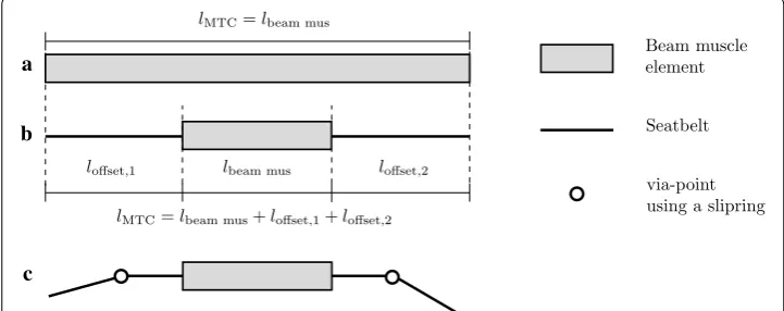
Muscle length offset and muscle routing
To enable physiological muscle path representation for the extended Hill-type muscle model several routing methods could be considered. In advanced modelling frameworks the muscle path is usually redirected either by specific points, so called via-points, or by surfaces of geometrical objects (e.g. in OpenSim [32]). See [33] additionally for an (22) ˙
q= 1
τact
STIM−STIM1−βq(q−q0)−βq(q−q0).
(23) q= q0+(ρ·γrel)
3
1+(ρ·γrel)3
.
(24) ˙
γrel=m(STIM−γrel), withγrel(t0)=0 ,
(25) ρ=c·η (k−1)
in-depth review and comparison of routing methods in biomechanical models. It was decided to use the via-point approach as described in [20], because it is possible to implement this method with the standard routing elements available for seatbelts in LS-DYNA. This method has proven to be reliable, as it is used in almost every crash simulation involving occupant models. To implement this, it is necessary to divide the MTC into muscle element and seatbelt elements, as only the latter can be routed. There-fore, an offset in length loffset is introduced, defined as the difference between the actual length of the muscle beam element length lbeam,mus in the model and the length of the entire MTC lMTC:
If necessary an offset can be added on both ends of the muscle beam element, to allow for two or more via-points, see Fig. 2. Standard seatbelt elements can be attached to the end of the muscle beam element and all the standard routing methods of LS-DYNA e.g. sliprings can be used. The seatbelt elements can move through a slipring node freely, while at the same time, the muscle model internally works with the correct length and dynamics of the entire MTC. To preserve the muscle dynamics it is required, that the stiffness of the seatbelt elements is orders of magnitude higher compared to the stiffness of the muscle elements. For the example in "Application in the ViVA OpenHBM Arm with routing" a stiffness of 1×10⁶ N/m was used for the seatbelt elements.
LS‑DYNA implementation
It is possible to include self-written code in the LS-DYNA FE solver through so-called ‘User Subroutines’. These subroutines have to be written in FORTRAN and can, among other options, be used to define user materials [24]. The muscle model described in "Muscle model" was implemented in LS-DYNA as a user material for truss elements (26)
lMTC=lbeam,mus+loffset
=lbeam,mus+loffset,1+loffset,2.
loffset,1 lbeam mus loffset,2
lMTC=lbeam mus
a
b
c
Beam muscle element
Seatbelt
via-point using a slipring
lMTC=lbeam mus+loffset,1+loffset,2
to simulate the active contraction behaviour, as well as the passive spring and damp-ing effects of human muscles. The FORTRAN code is available at https://zenodo.org/ record/826209.
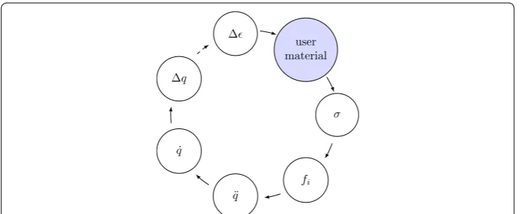
The explicit integration scheme in LS-DYNA, shown in Fig. 3, is updating the element strain �ǫ in each timestep based on the nodal displacement u. Material models trans-late the strain �ǫ to stress σ, which yield nodal forces fi. These forces result in nodal acceleration u¨, which are integrated to nodal velocity u˙ and displacement u for the next timestep.
It should be pointed out, that material subroutines require an element stress as a return value. In the concept of the muscle model, only forces are calculated. Since truss elements can only have axial stress, the stress was calculated from the muscle force and the element cross-section area via
If the material card for user-defined material models is specified in an input deck, LS-DYNA internally calls the routine usrmat, which starts the corresponding element rou-tine, depending on the element type. In the case of beam elements this is urmatb and for truss elements urmatt. Finally, the actual material routine is called, which the user can program himself. It is possible to have up to ten user materials defined in the sub-routines umat41 to umat50. The user can implement arbitrary material models in these routines and, among other things, access the material parameters specified in the mate-rial card. In addition, the programmer may call further subroutines, which then return, for example, nodal coordinates or various element properties.
Verification and validation set‑up
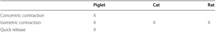
For the Hill-type model parameters identification, a general test procedure requires three experimental set-ups: (a) concentric contraction, (b) isometric contraction and (c) quick release [12]. They are depicted in Fig. 4 and explained in detail below. A com-plete set of muscle parameters is almost never found in a single source since it is hard
(27) σ = FMTC
A .
σ
user material ∆
∆q
˙
q
¨
q
fi
to perform all three tests in a row with the same muscle specimen, so a short literature survey is always required.
The validation conducted for the muscle model is based on mammalian muscle experi-ments. As there is no experimental data available for actual human muscle tissue, the model validation is based on piglet [16], cat [34] and rat [35] muscle experiments. The verification is done in comparison with an already existing implementation of the same muscle model in the Matlab based multi-body code Neweul-M2 [36]. Additionally, a comparison with the *MAT_156 muscle material from LS-DYNA is shown for the con-centric contraction experiment. Data sets from all three experimental set-ups are avail-able for the piglet muscle. For the other two species, a specific set-up for an isometric contraction experiment is applied, which was shown to be sufficient to determine all necessary Hill-type parameters for simulations [37]. An overview of all experimental set-ups is presented in Table 1. Furthermore all model parameters are given in tabular form for each validation case including references.
Concentric contraction experiment
In a concentric contraction, the muscle is shortened, which means that the dis-tance between muscle origin and insertion point decreases, e.g. elbow flexion to lift a weight, see Fig. 4a. In the simulation set-up, the muscle element is orientated vertically and the upper node is fixed. Masses between m=0.1 kg and m=1.8 kg are attached to the lower node in accordance with the experimental studies. At the beginning of the test, the muscle is relaxed and the mass is resting on a plane. Then the muscle is
a b c
m m
g
Fig. 4 Illustration of the a concentric and b isometric contraction and the c quick release experiments
Table 1 Overview of all set-ups used for validation
Piglet Cat Rat
Concentric contraction X
Isometric contraction X X X
stimulated (STIM=1) and starts to contract. At first no external motion is recorded as only the internal length lCE is decreasing. Once FMTC>FGravity the mass is lifted and the contraction velocity is recorded and compared to the experimental results from the piglet muscles.
Isometric contraction experiment
In an isometric contraction the muscle force is increased, while the length of the muscle is kept constant, see Fig. 4b. This contraction mode occurs, for example, when attempt-ing to hold a heavy weight. In the simulation set-up both nodes of the muscle element are fixed. At the beginning of the test, there is no stimulation (STIM=0), thus the mus-cle experiences only a minimal activity q0. Starting from 0.1 s, the muscle is stimulated completely (STIM=1) and relaxed again completely after 1.1 s (STIM=0) in the pig-let [16] and cat [34] experiments. In the rat experiments the muscle is only activated for a shorter time period of 300 ms [35]. In the piglet muscle experiments the isometric contraction was carried out for different fixed muscle lengths between 5.1 and 6.6 cm around the anatomical resting length of lMTC,0=lCE,opt+lSEE,0. In the other experi-ments the isometric contraction was only tested for the anatomical resting length. In the results, the force vs. time curves are compared and also the differences resulting from the two activation dynamics implemented are analyzed.
Quick release experiment
The quick release is a combination of isometric and concentric contraction. In this set-up, the muscle is fixed at both ends at the beginning, it is then stimulated (STIM = 1) and isometric contraction occurs Fig. 4c. After 1 s the lower end of the muscle carrying a mass is released and is pulled up quickly due to the force built up during the isometric contraction. After a total time of 1.5 s the stimulation is switched off again (STIM = 0). As in the concentric case, the influence of the different masses is examined (m= 200, 400, 600, 800, 1000, and 1500 g) for the piglet muscles only [16].
Simulation results
The verification and validation simulation results are shown in the following sections for piglet, rat and cat muscles. Using the piglet data, an additional comparison to the mus-cle model *MAT_156 already existing in LS-DYNA is shown and the differences result-ing from the two distinctive muscle activation dynamics implemented are illustrated. To demonstrate the application of the model in AHBMs an example illustrating the routing capabilities is given using an elbow model extracted from the ViVA OpenHBM [3].
Piglet calf muscle
Concentric contraction
The numerical and experimental results are presented in Fig. 5. All curves are shifted in time so that the mass is pulled up or FMTC=FGravity occurs at t=0 s. As shown in the figure, the simulation results from LS-DYNA are very consistent with the experi-ments and the simulations with the muscle model in Neweul-M2. A comparison with the simulation data from [16] would give even better results. The differences between the simulation results from Neweul-M2 and LS-DYNA can presumably be attributed to dif-ferent computational accuracies and integration methods for the difdif-ferential equations. These simulations were both run with explicit integrators and a constant time step. Con-sequently, we can state that we have a correct muscle model implementation for the con-centric contraction case.
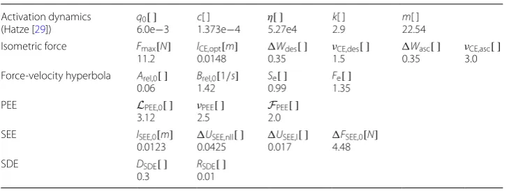
In addition a comparison with the muscle material model *MAT_156, already existing in LS-DYNA, is shown in Fig. 6. The initial contraction velocity provides similar results. Also, the maximum force value for low masses up to about 200 g is well approximated. The *MAT_156 material, however, shows significant weaknesses in speed decay and in the correct representation of the damping properties. At this point, it should be noted Table 2 Muscle parameters for the piglet simulations. See [16, Table 2, p. 68]
Activation dynamics
(Zajac [11]) q1.0e0[ ]−4 τq0.025[s] βq0.5[ ] Activation dynamics
(Hatze [29])
q0[ ]
5.0e−3 c1.373e[ ] −4 η5.27e[ ] −4 k2.9[ ] m11.3[ ] Isometric force Fmax[N]
30.0
lCE,opt[m]
0.015
Wdes[ ]
0.14 νCE,des
[ ]
3.0
Wasc[ ]
0.57 νCE,asc
[ ]
4.0 Force-velocity hyperbola Arel,0[ ]
0.1 Brel,01.0 [1/s] Se2.0[ ] Fe1.8[ ]
PEE LPEE,0[ ]
0.9 ν2.5PEE[ ]
FPEE[ ] 1.0
SEE lSEE,0[m]
0.045 0.1825USEE,nll[ ] 0.073USEE,l[ ] 60.0FSEE,0[N]
SDE DSDE[ ]
0.3 R0.01SDE[ ]
0 0.02 0.04 0.06 0.08 0.1 0.12 0.14 0.16 0
0.02 0.04 0.06 0.08 0.1 0.12
time [s]
con
traction
velo
cit
y
[m/s]
100 g 200 g 400 g 600 g 800 g 1400 g 1800 g
that further optimization of the material parameters might achieve better results. For these simulations the *MAT_156 parameters were derived from the previous work of [38]. This comparison shows the potential of the newly implemented muscle model and shows how it can help to deliver more realistic simulation results.
Isometric contraction
In Fig. 7 the numerical results for both the LS-DYNA and the Neweul-M2 simulations are depicted together with the experimental results. In the piglet experiments different
0 0.02 0.04 0.06 0.08 0.1 0.12 0.14 0.16 0
0.02 0.04 0.06 0.08 0.1 0.12
time [s]
con
traction
velo
cit
y
[m/s]
usermat *MAT 156
Fig. 6 Comparison of the concentric contraction velocity between the extended Hill-type muscle model and *MAT_156. Full line extended Hill-type muscle model, dashed line *MAT_156. Colours are identical to Fig. 5
0 0.1 0.2 0.3 0.4 0.5 0.6 0.7 0.8 0.9 1 1.1 1.2 1.3 1.4 1.5 0
5 10 15 20 25 30 35 40 45
time [s]
m
uscle
force
[N]
h= 0.85 h= 0.88 h= 0.91 h= 0.94 h= 1.00 h= 1.03 h= 1.08 h= 1.10
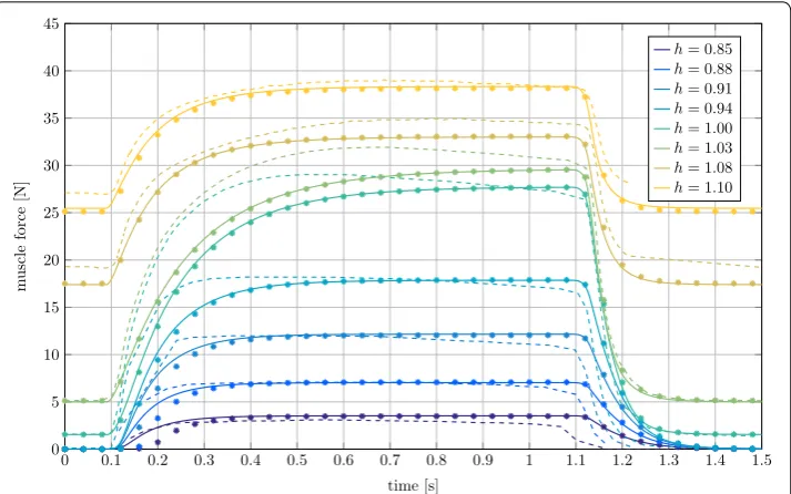
Fig. 7 Force output of the MTC plotted versus time for different fixed stretch ratios h in isometric contraction.
starting length of the MTC lMTC were tested. In Fig. 7 the tests are differentiated by the stretch ratio h=lMTC/lMTC,0 of the starting length and the anatomical resting length lMTC,0.
The comparison of the LS-DYNA results with the experimental data shows, that the muscle force for the inactive muscle in the time intervals t<0.1 s and t>1.1 s is underestimated if the muscle is lengthened considerably relative to the anatomical rest-ing length (h>1.05). Also, a clear deviation in the force increase for the stretch ratios h=1.0 and h=1.03 exists, while the final force at t=1 s is met. Very similar differ-ences are also present in the simulation results from [16]. According to this source, the proposed muscle model does not represent all internal dependencies of the Hill param-eters correctly. Also potential history effects visible in the experimental curves, namely non-steady force plateaus, are made responsible for the differences. Furthermore, pos-sible deficits in the identification of the parameters for the activation dynamics and the rise of FCE play a role. The comparison to Neweul-M2 shows high agreement with only slight deviations in the muscle activation interval for the ratios h=0.85, 0.88 and
0.91. As it was the case in the concentric contraction, the differences in the results are larger for higher dynamics, which can probably be attributed to the different integration method for solving the differential equations.
The most important point illustrated by the isometric contraction in Fig. 7 is the strong dependence of the maximum isometric force on the muscular length. This finding is decisive for the application in AHBMs, since in this example deviations of approxi-mately 15 mm in muscle length lead to differences in muscle force of more than 30 N.
Comparison of activation dynamics for isometric contraction
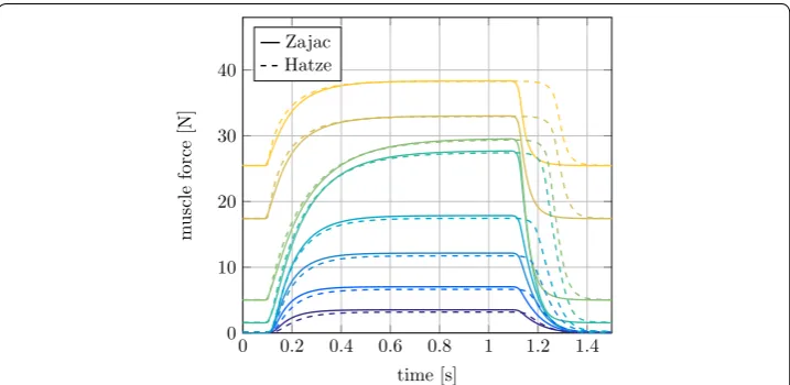
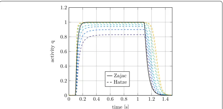
In the extended Hill-type muscle model two different approaches to describe the acti-vation dynamics are implemented. In Figs. 8 and 9 these methods by Zajac [11] and Hatze [29] are compared in an isometric contraction.
The muscle force results with Hatze and Zajac activation differ mainly during muscle deactivation after t=1.1 s, see Fig. 8. The forces of muscles with a high stretch ratio
0 0.2 0.4 0.6 0.8 1 1.2 1.4 0
10 20 30 40
time [s]
mu
scle
force
[N]
Zajac Hatze
decrease significantly later than the muscles that are shortened. The concentration of free Ca2+ ions γrel evolves similar to the activity level described by the differential equa-tion of Zajac. γrel increases slightly slower and takes about 0.1 s longer to decay. The
larger influence is the dependence of the activation on the CE length through ρ for
the Hatze activation dynamics, see Fig. 9. By stretching the muscle, lCE is significantly
longer for high h-ratios. As a result, ρ will increase and the activity is rising faster for the
stretched muscles. The stretch ratio and thus ρ also affect the maximum activity level
reached in the simulations. It can be seen in Fig. 9, that the maximum activity of the muscle with h=0.85 is only about 82%. For Zajac’s activation dynamics only one curve is found in Fig. 9, this is because Zajac’s activation dynamics is length-independent and therefore all activation curves are identical.
As the formulation of activation dynamics by Hatze is the more biofidelic and supe-rior option [37], the comparison for rat and cat experiments will be done only with this dynamics.
Quick release
The quick release experiments are a combination of the two experiments above. Here the force produced by the MTC is analyzed versus the contraction velocity. In Fig. 10 the numerical results from LS-DYNA and Neweul-M2 as well as the experimental data is shown.
The isometric muscle force at zero velocity, i.e. before the muscle is released, is about 2 N lower than in the experiments. However, the results clearly approach the respective maximum contraction velocities. In [16] it is stated, that this is due to history effects within the tendon in the experiments that are not represented in the muscle model. The best agreement is achieved for a mass of 1000 g, where according to [16] the history effects were absent. The difference with Neweul-M2 is once again negligibly small for the bigger masses and slightly larger for the high velocities or smaller masses.
0 0.2 0.4 0.6 0.8 1 1.2 1.4
0 0.2
0.4
0.6 0.8
1 1.2
time [s]
activit
yq
Zajac Hatze
Rat gastrocnemius medialis muscle
The experiments were done by Siebert et al [35] on the rat (Rattus norvegicus, Wistar) M. gastrocnemius medialis muscle. The parameters for the Hill-type muscle model are listed in [35, Table 4, p. 222] and the experimental set-up description is provided on page 218 of the same publication. Optimal Hatze activation dynamics parameters are listed in [37, Table 2, column 6, p. 278].
For convenience, they are collected in Table 3 and the LS-DYNA material card is given in Appendix "Material card for rat simulations". As seen in Fig. 11 the simulation results are in good agreement with the experimental results, being a little faster in the muscle deactivation slope.
Cat soleus muscle
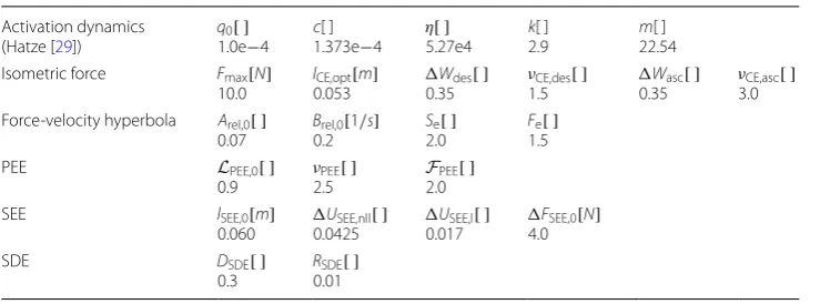
Mörl et al. [34] conducted the experiments on the cat soleus muscle. The parameters for the Hill-type muscle model are found in [34, Table 1, p. 5] with optimal Hatze activation
0 0.05 0.1 0.15 0.2 0.25 0.3 0.35 0.4 0.45 0.5
0 5 10 15 20 25 30
contraction velocity [m/s]
m
uscle
force
[N]
200 g 400 g 600 g 800 g 1000 g 1500 g
Fig. 10 Force output of the MTC plotted versus contraction velocity at different muscle loads in quick release experiments. Full line LS-DYNA, dots Neweul-M2, dashed line experimental results
Table 3 Muscle parameters for the rat simulations
Activation dynamics
(Hatze [29]) q6.0e0[ ]−3 1.373ec[ ] −4 η5.27e4[ ] k2.9[ ] m22.54[ ] Isometric force Fmax[N]
11.2
lCE,opt[m]
0.0148
Wdes[ ]
0.35 ν1.5CE,des[ ] Wasc[ ]
0.35 ν3.0CE,asc[ ] Force-velocity hyperbola Arel,0[ ]
0.06
Brel,0[1/s]
1.42
Se[ ]
0.99
Fe[ ]
1.35
PEE LPEE,0[ ]
3.12 ν2.5PEE[ ]
FPEE[ ]
2.0
SEE lSEE,0[m]
0.0123
USEE,nll[ ]
0.0425
USEE,l[ ]
0.017
FSEE,0[N]
4.48
SDE DSDE[ ]
0.3
RSDE[ ]
dynamics parameters once more taken from [37]. They are also collected in Table 4 and a material card for LS-DYNA is provided in Appendix "Material card for cat simulations". The corresponding simulation results depicted in Fig. 12, are in excellent agreement with the experimental results, this time being a little faster in the muscle activation slope.
Application in the ViVA OpenHBM Arm with routing
The extended Hill-type muscle model is applied in an arm model extracted from the ViVA OpenHBM [3]. The model includes bones, modelled as rigid bodies, and flexible flesh and skin of the upper extremity. We added the main flexors (biceps long and short heads, brachialis, brachioradialis, pronator teres and extensor carpi radialis) and exten-sors (triceps long, lateral and medial heads) of the elbow joint, which we idealized as a revolute joint. Here the via-point routing method is compared to simple direct line and lever approaches. Moreover a complete description of the set-up of the elbow model [39] and the choice of parameters for all muscles at the elbow [32] is out of scope for this publication.
The via-point method allows the selection of anatomical origin and insertion nodes for the muscles. As a result the modelled muscle length is almost identical to the anatomi-cal muscle-tendon length. This enables the usage of anatomianatomi-cal data from literature for
Table 4 Muscle parameters for the cat simulations
Activation dynamics
(Hatze [29]) q1.0e0[ ]−4 1.373ec[ ] −4 η5.27e4[ ] k2.9[ ] m22.54[ ] Isometric force Fmax[N]
10.0
lCE,opt[m]
0.053
Wdes[ ]
0.35 νCE,des1.5 [ ] Wasc[ ]
0.35 ν3.0CE,asc[ ]
Force-velocity hyperbola Arel,0[ ] 0.07
Brel,0[1/s] 0.2
Se[ ]
2.0
Fe[ ]
1.5
PEE LPEE,0[ ]
0.9 ν2.5PEE[ ]
FPEE[ ]
2.0
SEE lSEE,0[m]
0.060
USEE,nll[ ]
0.0425
USEE,l[ ]
0.017
FSEE,0[N]
4.0
SDE DSDE[ ]
0.3
RSDE[ ]
0.01
0 0.1 0.2 0.3 0.4 0.5 0.6
0 2 4 6 8 10 12
time [s]
mu
scle
force
[N]
simulation experiment
the muscle parameters. The routing is done in LS-DYNA using sliprings fixed to bones in certain positions in space. The routing parameters, i.e. the offset length of the muscle and the position of the via-point, can be chosen independently of the muscle parame-ters to match the anatomy. This approach makes it possible to model the muscle-tendon dynamics correctly and at the same time making the lever arm vs. joint angle curve and thus the resulting elbow torque more realistic.
In Fig. 13 different strategies for modeling the triceps are shown. A direct line of action approach, lever arms of 10 and 20 mm, and the via-point routing method are shown. In contrast to the other methods, the application of the via-point method can deliver cor-rect lever arms for the complete range of motion of the elbow and fits the experimental corridor from [40] best, see Fig. 14. Additionally, the proposed via-point routing method improves the numerical stability of the model as it provides correct force application directions. Most importantly, the muscle dynamics is independent from the actual length of the combined elements (muscle + seatbelt, Fig. 2) and their path complexity
0 0.2 0.4 0.6 0.8 1 1.2 1.4 0
2 4 6 8 10 12
time [s]
m
uscle
force
[N]
simulation experiment
Fig. 12 Isometric experimental and simulation results for a cat muscle
rigid joint
via–point lever
bones centre
fixed to humerus muscles
in FE AHBMs. This is because of the separation of muscle and routing parameters in the FE model.
In comparison with the LS-DYNA *MAT_156 muscle model a 10 times speed-up is achieved for the validation simulations with one single muscle elements. As this set-up is clearly not very realistic, the ViVA arm simulations are repeated with *MAT_156 muscles to be comparable to the simulations with the extended Hill-type muscles. Here no speed-up is achieved, since most of the CPU time is used for the processing of the volumetric elements and the time needed to process truss elements is insignificant in comparison.
Conclusion and outlook
The upcoming challenges in the field of automotive safety, namely active safety systems and autonomous driving, will require and benefit greatly from AHBMs. The Hill-type muscle model already existing in LS-DYNA has a limited accuracy because it lacks an internal degree of freedom and in addition is difficult to parameterize. Here, an extended Hill-type muscle model was implemented, verified and validated successfully. The source code, parameters and an example set-up for LS-DYNA are provided at https://zenodo. org/record/826209. The verification and validation was done in comparison with experi-mental data sets from piglet, cat and rat muscles. The results are in very good agree-ment with the experiagree-ments and the new muscle model improves the accuracy available for AHBMs in LS-DYNA considerably. Moreover, the muscle model incorporates the activation dynamics, essential for correct simulations on small time horizons of dynamic active movements. Additionally, a convenient option for routing the muscle around joints was proposed. By introducing an offset to the length of the muscle element, it is possible to route the muscle using e.g. the via-point method, while at the same time the
20 40 60 80 100 120
−40 −30 −20 −10 0 10
elbow angle [°]
le
ve
r
arm
triceps
[mm]
direct line via–point 10 mm lever 20 mm lever exp. corridor
muscle will display the correct dynamics of the full muscle. This also means, that the parameters for the muscle model can be set independently of the routing.
Although the current model allows to predict the gross dynamic contraction charac-teristics of biological muscles, it has its limitations. For one, it is a force element predict-ing a scalar force value which is then applied between origin and insertion, or redirected by via-points. Contact forces and resulting shifts in the force direction or their influence on the active muscle force [35] are neglected. Besides that, several physiological effects of the muscle contraction are currently not considered, starting with muscle-morphol-ogy specific parameters such as the pennation angle [41] or the fibre composition [42]. Also on the dynamic level, e.g., modelling the force-velocity relation for the eccentric (lengthening) contractions is difficult, as little data is available. Some of the data sug-gests more complex relations than modelled here for extensive strains [43], which, how-ever, are not reached in our simulations. Furthermore, the experimentally found history effects causing force enhancement and force depression after stretch and shortening are currently not considered, but may be included in more extended approaches [44, 45]. Finally, the muscles model considers no mass or mass distribution, which, however, plays a role in dynamic contractions [46].
To utilize the full potential of the AHBMs, a control strategy for the activation of the muscles is needed. As a controller realization is not in the scope of this work, the authors recommend the review by [47] as a reliable source of information for muscle activations schemes and strategies in AHBMs. In principle, controllers are required which either maintain a desired position against perturbations or allow for the generation of a desired movement. Such controllers can be implemented in the current framework and may be easily added to the code provided in the Appendix.
With this, we provide a comprehensive and valid approach to implement an extended Hill-type muscle model in LS-DYNA, including muscle-tendon properties, biochemical activation dynamics, and muscle routing. By providing the code and the material cards, we hope that this will allow other researchers to work on more biofidelic AHBMs. Authors’ contributions
CK and OM were the major contributors in writing the manuscript, creating the illustrations and doing the simulations. JP, supervised by JF, wrote the FORTRAN code for the user-defined material and set up initial simulation models. DH, SSc and other colleagues developed the muscle model originally in Matlab and C code. SSc provided the approach for the muscle routing, the concept for the offset length was developed by JP and CK. DH, JF and SS contributed to the publica-tion as such, the open-source idea and in solving implementapublica-tion issues. Their revisions and important input improved the publication. All authors read and approved the final manuscript.
Author details
1 Institute for Engineering and Computational Mechanics, University of Stuttgart, Pfaffenwaldring 9, 70569 Stuttgart, Germany. 2 Biomechanics and Biorobotics, Stuttgart Research Centre for Simulation Sciences (SRC SimTech), University of Stuttgart, Allmandring 28, 70569 Stuttgart, Germany. 3 Multi-Level Modeling in Motor Control and Rehabilitation Robotics, Hertie Institute for Clinical Brain Research, University of Tübingen, Otfried-Müller-Strasse 25, 72076 Tübingen, Germany.
Acknowledgements
Competing interests
The authors declare that they have no competing interests. Availability of data and materials
The source code of the extended Hill-Type Muscle Model for LS-DYNA, an example and all simulation results are available at doi:10.5281/zenodo.826209. The original Matlab code of the muscle model can be found at doi:10.5281/ zenodo.439513.
Consent for publication Not applicable.
Ethics approval and consent to participate Not applicable.
Funding
This work was supported by Daimler AG through Tech Center i-protect, DFG through Exzellenzcluster 310 Simulation-stechnik and Ministry of Science, Research and the Arts Baden-Württemberg through project Az:33-7533.-30-20/7/2. This support is gratefully acknowledged and appreciated.
Appendix A: LS-DYNA material cards for validation simulations
In the following sections, the material cards for the simulations of the piglet, cat and rat muscles are given in the SI unit system. The simulations were set up with single muscle elements with a length of lMTC=lCE,opt+lSEE0 where applicable. The parameters are taken from [14, 16, 25, 29, 34, 35, 37]. LS-DYNA uses the density, bulk modulus and shear modulus to determine the time-step for the simulation. The density was set to 1×10⁻⁶ kg m−3 and the bulk modulus and shear modulus were adjusted to achieve a time-step smaller than 1×10⁻⁴ s.
Material card for piglet simulations
*MAT_USER_DEFINED_MATERIAL_MODELS
$ Hill-type Muscle for piglet muscle guentherschmittwank07
$#1 mid ro mt lmc nhv iortho ibulk ig
1 1.0000E-6 41 32 15 0 31 32
$#2 ivect ifail itherm ihyper ieos lmca unused unused
0 0 0 0 0 0
$#3 ActOpt STIM_ID q0 tauq/c betaq/eta k m lOffset
1 3 1.0E-4 0.025 0.5 0
$#4 Fmax lCEopt dWdes nuCEdes dWasc nuCEasc Arel0 Brel0
30.0 0.015 0.14 3.0 0.57 4.0 0.1 1.0
$#5 Secc Fecc LPEE0 nuPEE FPEE lSEE0 dUSEEnll duSEEl
2.0 1.8 0.9 2.5 1.0 0.045 0.1825 0.073
$#6 dFSEE0 Damping Param1 Param2 Output dtOut IBULK IG
Material card for rat simulations
*MAT_USER_DEFINED_MATERIAL_MODELS
$ Hill-type Muscle for a rat gm siebert14
$#1 mid ro mt lmc nhv iortho ibulk ig
1 1.0000E-6 41 32 15 0 31 32
$#2 ivect ifail itherm ihyper ieos lmca unused unused
0 0 0 0 0 0
$#3 ActOpt STIM_ID q0 tauq/c betaq/eta k m lOffset
2 3 0.006 1.373E-4 5.27E4 2.9 22.54 0
$#4 Fmax lCEopt dWdes nuCEdes dWasc nuCEasc Arel0 Brel0
11.2 0.0148 0.35 1.5 0.35 3.0 0.06 1.42
$#5 Secc Fecc LPEE0 nuPEE FPEE lSEE0 dUSEEnll duSEEl
0.99 1.35 3.12 2.5 2.0 0.0123 0.0425 0.017
$#6 dFSEE0 Damping Param1 Param2 Output dtOut IBULK IG
4.48 3.0 0.3 0.01 1 0 0.13 0.13
Material card for cat simulations
*MAT_USER_DEFINED_MATERIAL_MODELS
$ Hill-type Muscle for a cat soleus moerl12
$#1 mid ro mt lmc nhv iortho ibulk ig
1 1.0000E-6 41 32 15 0 31 32
$#2 ivect ifail itherm ihyper ieos lmca unused unused
0 0 0 0 0 0
$#3 ActOpt STIM_ID q0 tauq/c betaq/eta k m lOffset
2 3 1.0E-4 1.373E-4 5.27E4 2.9 22.54 0
$#4 Fmax lCEopt dWdes nuCEdes dWasc nuCEasc Arel0 Brel0
10.0 0.053 0.35 1.5 0.35 3.0 0.07 0.2
$#5 Secc Fecc LPEE0 nuPEE FPEE lSEE0 dUSEEnll duSEEl
2.0 1.5 0.9 2.5 2.0 0.060 0.0425 0.017
$#6 dFSEE0 Damping Param1 Param2 Output dtOut IBULK IG
4.0 3.0 0.3 0.01 1 0 0.13 0.13
Appendix B: Material cards description and corresponding symbols
Card 1 1 2 3 4 5 6 7 8
Variable MID RO MT LMC NHV IORTH IBULK IG
Default – 1E-6 41 32 15 0 31 32
Variable Description
MID Material identification. A unique number or label not exceeding eight characters must be specified RO∗† Mass density. Not used by the material model
MT User material type. In this case 41 must be defined LMC Length of material constant array. For this material 32
must be set
NHV Number of history variables to be stored. 15 are required for this material
IORTH EQ.1: if the material is orthotropic
EQ.2: if material is used with spot weld thinning EQ.3: if material is orthotropic and used with spot weld
thinning
IBULK Adress of bulk modulus in material constants array IG Adress of shear modulus in material constants array
Card 2 1 2 3 4 5 6 7 8
Variable IVECT IFAIL ITHERM IHYPER IEOS LMCA
Default 0 1 - – – – –
Variable Description
IVECT Vectorization flag (on = 1). A vectorized user subroutine must be supplied
IFAIL Failure flag
EQ.0: No failure
EQ.1: Allows failure of shell and solid elements LT.0: |IFAIL| is the address of NUMINT in the material
constants array
ITHERM Temperature flag (on = 1). Compute element tempera-ture
IHYPER Deformation gradient flag (on = 1 or −1, or 3). Compute deformation gradient, see LSTC Appendix A: LS-DYNA material cards for validation simulations
IEOS Equation of state (on = 1)
LMCA Length of additional material constant array
Card 3 1 2 3 4 5 6 7 8
Variable Act STIM q0 tauq/c bq/eta k m lOffset
Default – – – – – – – 0
Variable Symbol Description
Act EQ.0.0: Input of activation values
EQ.1.0: Calculation of activation with Zajac depending on stimulation EQ.2.0: Calculation of activation with
Hatze depending on stimulation
STIM STIM LT.0.0: Constant stimulation or
activa-tion level. Depending on Act GT.0.0: LCID specifing the stimulation
Variable Symbol Description
q0 q0 Minimum value of activation q
tauq † / c τq / c If ACT.EQ.1.0: time constant of rising activation
If ACT.EQ.2.0: Hatze constant c
bq / eta βq/ η If ACT.EQ.1.0: ratio between τq and time constant of falling activation If ACT.EQ.2.0: Hatze constant η
k k If ACT.EQ.2.0: Hatze constant k
m m If ACT.EQ.2.0: Hatze constant m
lOffset † lOffset Muscle length offset added to beam
length before calculation of the muscle. lMTC,i=lBeam,i+lOffset
Card 4 1 2 3 4 5 6 7 8
Variable Fmax lCEopt dWdes nCEd dWasc nCEa Arel0 Brel0
Default – – – – – – – –
Variable Symbol Description
Fmax † Fmax Maximum isometric force
lCEopt † lCE,opt Optimal fibre length
dWdes Wdes Width of Fisom(lCE) on descending
limb
nCEd νCE,des Exponent of Fisom(lCE) on
descend-ing limb
dWasc Wasc Width of Fisom(lCE) on ascending limb
nCEa νCE,asc Exponent of Fisom(lCE) on ascending
limb
Arel0 Arel,0 Maximum value of Arel
Brel0 † Brel,0 Maximum value of Brel
Card 5 1 2 3 4 5 6 7 8
Variable Secc Fecc LPEE0 nPEE FPEE lSEE0 dUSnll dUSl
Default – – – – – – – –
Variable Symbol Description
Secc Se Step in inclination of FCE(˙lCE=0)
between eccentric and concentric force-velocity relations
Fecc Fe Coordinate of pole in lCE(FCE)
normal-ised to FmaxqFisom(lCE) for lCE>0
LPEE0 LPEE,0 Rest length of PEE normalised to
lCE,opt
nPEE νPEE Exponent of FPEE(lCE)
FPEE FPEE Force of PEE if lCE is stretched to Wdes
lSEE0 † lSEE,0 Rest length of SEE
USnll USEE,nll Relative stretch at non-linear-linear
transition in FSEE(lSEE)
duSl USEE,l Relative stretch in linear part for force
Card 6 1 2 3 4 5 6 7 8
Variable dFSEE0 Damp Damp1 Damp2 Output dtOut IBULK∗ IG∗
Default - 3 - - 0 0 -
-Variable Symbol Description
dFSEE0 † FSEE,0 Force at non-linear-linear transition
in FSEE(lSEE)
Damp EQ.1.0: parallel damping
EQ.2.0: Serial damping
EQ.3.0: Serial force dependent damp-ing
Else: No damping
Damp1 dPE† If Damp.EQ.1.0: damping coefficient
of PE
dSE† If Damp.EQ.2.0: damping coefficient of SE
DSDE If Damp.EQ.3.0: dimensionless factor to scale dSE,max
Damp2 RSDE If Damp.EQ.3.0: minimum value of dSE
normalised to dSE,max
Output Definition of desired output content
of outputfile fort.(idele) for each muscle element:
EQ.0. no outputfile
EQ.1. basic output (idele, tt, ncycle, q) EQ.2. basic output and force data (idele...,FMTC,FSEE,FSDE,FCE,FPEE,Fisom)
EQ.-1. basic output and length data
(idele...,lMTC,lCE,˙lMTC,˙lCE)
EQ.-2. basic output and force and length data
(idele...,FMTC...,lMTC...)
dtout † Timestep of outputile fort.(idele)
IBULK∗ Bulk modulus. Needed by LS-DYNA
to calculate time-step automatically
IG∗ Shear modulus. Needed by LS-DYNA
to calculate time-step automatically
Publisher’s Note
Springer Nature remains neutral with regard to jurisdictional claims in published maps and institutional affiliations.
Received: 10 April 2017 Accepted: 21 August 2017
References
1. Iwamoto M, Omori K, Kimpara H, Nakahira Y, Tamura A, Watanabe I, Miki K, Hasegawa J, Oshita F, Nagak A. Recent advances in THUMS: development of individual internal organs, brain, small female and pedestrian model. In: Proceedings of 4th European LS Dyna users conference, Ulm, Germany; 2003. pp. 1–10.
2. Gayzik FS, Moreno DP, Vavalle NA, Rhyne AC, Stitzel JD. Development of a full human body finite element model for blunt injury prediction utilizing a multi-modality medical imaging protocol. In: Proceedings of the 12th Interna-tional LS-DYNA user conference, Dearborn, MI, USA; 2012.
4. Feller L, Kleinbach C, Fehr J, Schmitt S. Incorporating muscle activation dynamics into the Global Human Body Model. In: Proceedings of the IRCOBI conference, Malaga, Spain; 2016.
5. Shelat C, Ghosh P, Chitteti R, Mayer C. “Relaxed” HBM–an enabler to pre-crash safety system evaluation. In: Proceed-ings of the IRCOBI conference, Malaga, Spain; 2016.
6. Van Ee CA, Chasse AL, Myers BS. Quantifying skeletal muscle properties in cadaveric test specimens: effects of mechanical loading, postmortem time, and freezer storage. Trans Am Soc Mech Eng J Biomech Eng. 2000;122(1):9–14.
7. Östh J, Brolin K, Bråse D. A human body model with active muscles for simulation of pretensioned restraints in autonomous braking interventions. Traffic Inj Prev. 2015;16:304–13. doi:10.1080/15389588.2014.931949. 8. Iwamoto M, Nakahira Y. Development and validation of the Total HUman Model for Safety (THUMS) version 5
con-taining multiple 1d muscles for estimating occupant motions with muscle activation during side impacts. Stapp Car Crash J. 2015;59:53–90.
9. Livermore Software Technology Corporation: LS-DYNA Theory Manual. Livermore Software Technology Corporation; 2006
10. Audu ML, Davy DT. The influence of muscle model complexity in musculoskeletal motion modeling. J Biomech Eng. 1985;107:147–57.
11. Zajac FE. Muscle and tendon: properties, models, scaling, and application to biomechanics and motor control. Crit Rev Biomed Eng. 1989;17(4):359–411.
12. Winters JM. Hill-based muscle models: a systems engineering perspective. In: Winters JM, Woo SL-Y, editors. Multiple muscle systems. New York: Springer; 1990. pp. 69–93. doi:10.1007/978-1-4613-9030-5_5.
13. Wittek A, Kajzer J, Haug E. Hill-type muscle model for analysis of mechanical effect of muscle tension on the human body response in a car collision using an explicit finite element code. JSME Int J Ser A. 2000;43(1):8–18. doi:10.1299/ jsmea.43.8.
14. Siebert T, Rode C, Herzog W, Till O, Blickhan R. Nonlinearities make a difference: comparison of two common Hill-type models with real muscle. Biol Cybern. 2008;98(2):133–43. doi:10.1007/s00422-007-0197-6.
15. Mörl F, Siebert T, Häufle D. Contraction dynamics and function of the muscle-tendon complex depend on the muscle fibre-tendon length ratio: a simulation study. Biomech Model Mechanobiol. 2016;15(1):245–58. doi:10.1007/ s10237-015-0688-7.
16. Günther M, Schmitt S, Wank V. High-frequency oscillations as a consequence of neglected serial damping in Hill-type muscle models. Biol Cybern. 2007;97(1):63–79. doi:10.1007/s00422-007-0160-6.
17. Romero F, Alonso FJ. A comparison among different Hill-type contraction dynamics formulations for muscle force estimation. Mech Sci. 2016;7(1):19–29. doi:10.5194/ms-7-19-2016.
18. Nussbaum MA, Chaffin DB, Rechtien CJ. Muscle lines-of-action affect predicted forces in optimization-based spine muscle modeling. J Biomech. 1995;28:401–9. doi:10.1016/0021-9290(94)00078-I.
19. Günther M. Computersimulationen zur Synthetisierung des muskulär erzeugten menschlichen Gehens unter Verwendung eines biomechanischen Mehrkörpermodells. PhD thesis, Eberhard-Karls-Universität zu Tübingen, 1997. 20. Delp SL, Loan JP, Hoy MG, Zajac FE, Topp EL, Rosen JM. An interactive graphics-based model of the lower extremity
to study orthopaedic surgical procedures. IEEE Trans Biomed Eng. 1990;37(8):757–67. doi:10.1109/10.102791. 21. Günther M, Ruder H. Synthesis of two-dimensional human walking: a test of the lambda-model. Biol Cybern.
2003;89:89–106. doi:10.1007/s00422-003-0414-x.
22. Favre P, Gerber C, Snedeker JG. Automated muscle wrapping using finite element contact detection. J Biomech. 2010;43(10):1931–40. doi:10.1016/j.jbiomech.2010.03.018.
23. Erhart T. Pulley mechanism for muscle or tendon movements along bones and around joints. In: German LS-DYNA Forum 2012. DYNAmore GmbH. https://www.dynamore.de/de/download/papers/ls-dyna-forum-2012/documents/ passive-3-3/at_download/file. 2012.
24. Livermore Software Technology Corporation. LS-DYNA Keyword User’s Manual Volume I, LS-DYNA R8.0 03/23/15 (r:6319). Livermore: Livermore Software Technology Corporation; 2015.
25. Haeufle DFB, Günther M, Bayer A, Schmitt S. Hill-type muscle model with serial damping and eccentric force-veloc-ity relation. J Biomech. 2014;47(6):1531–6. doi:10.1016/j.jbiomech.2014.02.009.
26. Hill AV. The heat of shortening and the dynamic constants of muscle. Proc R Soc Lond Ser B Biol Sci. 1938;126(843):136–95. doi:10.1098/rspb.1938.0050.
27. Schmitt S: Über die Anwendung und Modifikation des Hillschen Muskelmodells in der Biomechanik. PhD thesis, Eberhard-Karls-Universitat, Tubingen, 2006.
28. Bayer A, Schmitt S, Günther M, Haeufle D. The influence of biophysical muscle properties on simulating fast human arm movements. Comput Methods Biomech Biomed Eng. 2017;20(8):803–21. doi:10.1080/10255842.2017.1293663. 29. Hatze H. A general myocybernetic control model of skeletal muscle. Biol Cybern. 1978;28(3):143–57. doi:10.1007/
BF00337136.
30. Rassier DE, Herzog W. Length dependence of force production and Ca2+ sensitivity in skeletal muscle. In: Herzog W, editor. Skeletal muscle mechanics : from mechanisms to function. Chichester: Wiley; 2000. p. 71–88.
31. Kistemaker DA, Van Soest AKJ, Bobbert MF. Length-dependent [Ca2+] sensitivity adds stiffness to muscle. J Biomech. 2005;38(9):1816–21. doi:10.1016/j.jbiomech.2004.08.025.
32. Holzbaur KRS, Murray WM, Delp SL. A model of the upper extremity for simulating musculoskeletal surgery and analyzing neuromuscular control. Ann Biomed Eng. 2005;33(6):829–40. doi:10.1007/s10439-005-3320-7. 33. Hwang J, Knapik GG, Dufour JS, Marras WS. Curved muscles in biomechanical models of the spine: a systematic
literature review. Ergonomics. 2017;60(4):577–588. doi:10.1080/00140139.2016.1190410.
34. Mörl F, Siebert T, Schmitt S, Blickhan R, Günther M. Electro-mechanical delay in Hill-type muscle models. J Mech Med Biol. 2012;12(05):1250085–1125008518. doi:10.1142/S0219519412500856.
35. Siebert T, Till O, Blickhan R. Work partitioning of transversally loaded muscle: experimentation and simulation. Com-put Methods Biomech Biomed Eng. 2014;17(3):217–29. doi:10.1080/10255842.2012.675056.
• We accept pre-submission inquiries
• Our selector tool helps you to find the most relevant journal • We provide round the clock customer support
• Convenient online submission • Thorough peer review
• Inclusion in PubMed and all major indexing services • Maximum visibility for your research
Submit your manuscript at www.biomedcentral.com/submit
Submit your next manuscript to BioMed Central
and we will help you at every step:
37. Rockenfeller R, Günther M. Extracting low-velocity concentric and eccentric dynamic muscle properties from isometric contraction experiments. Math Biosci. 2016;278:77–93. doi:10.1016/j.mbs.2016.06.005.
38. Schmitt S, Blaschke J, Böhm P, Mayer C. Active muscles for the implementation in human body models-work in progress. In: Proceedings of the IRCOBI conference, Lyon, France. International Research Council on Biomechanics of Injury (IRCOBI); 2015. pp. 648–649.
39. Fehr J, Kempter F, Kleinbach C, Schmitt S. Guiding strategy for an open source Hill-type muscle model in LS-DYNA and implementation in the upper extremity of a HBM. In: Proceedings of the IRCOBI conference, Antwerp, Belgium; 2017.
40. Murray WM, Buchanan TS, Delp SL. Scaling of peak moment arms of elbow muscles with upper extremity bone dimensions. J Biomech. 2002;35(1):19–26. doi:10.1016/S0021-9290(01)00173-7.
41. Elias LA, Watanabe RN, Kohn AF. Spinal mechanisms may provide a combination of intermittent and continuous control of human posture: predictions from a biologically based neuromusculoskeletal model. PLOS Comput Biol. 2014;10(11):1–18. doi:10.1371/journal.pcbi.1003944.
42. Cheng EJ, Brown IE, Loeb GE. Virtual muscle: a computational approach to understanding the effects of muscle properties on motor control. J Neurosci Methods. 2000;101(2):117–30. doi:10.1016/S0165-0270(00)00258-2. 43. Tomalka A, Rode C, Schumacher J, Siebert T. The active force–length relationship is invisible during extensive
eccentric contractions in skinned skeletal muscle fibres, vol. 284. London: The Royal Society; 2017. doi:10.1098/ rspb.2016.2497. http://rspb.royalsocietypublishing.org/content/284/1854/20162497.
44. McGowan CP, Neptune RR, Herzog W. A phenomenological muscle model to assess history dependent effects in human movement. J Biomech. 2013;46(1):151–7. doi:10.1016/j.jbiomech.2012.10.034.
45. Rode C, Siebert T, Blickhan R. Titin-induced force enhancement and force depression: a ’sticky-spring’ mechanism in muscle contractions? J Theor Biol. 2009;259(2):350–60. doi:10.1016/j.jtbi.2009.03.015.
46. Günther M, Röhrle O, Haeufle DFB, Schmitt S. Spreading out muscle mass within a Hill-type model: a computer simulation study. Comput Math Methods Med. 2012;2012:848630. doi:10.1155/2012/848630.
![Table 2 Muscle parameters for the piglet simulations. See [16, Table 2, p. 68]](https://thumb-us.123doks.com/thumbv2/123dok_us/9105391.1903209/13.595.118.477.529.698/table-muscle-parameters-piglet-simulations-table-p.webp)