Geosci. Model Dev., 5, 1273–1295, 2012 www.geosci-model-dev.net/5/1273/2012/ doi:10.5194/gmd-5-1273-2012
© Author(s) 2012. CC Attribution 3.0 License.
Geoscientific
Model Development
Description of a hybrid ice sheet-shelf model, and application to
Antarctica
D. Pollard1and R. M. DeConto2
1Earth and Environmental Systems Institute, Pennsylvania State University, University Park, PA, USA 2Department of Geosciences, University of Massachusetts, Amherst, MA, USA
Correspondence to: D. Pollard ([email protected])
Received: 2 April 2012 – Published in Geosci. Model Dev. Discuss.: 4 May 2012 Revised: 3 August 2012 – Accepted: 4 September 2012 – Published: 17 October 2012
Abstract. The formulation of a 3-D ice sheet-shelf model is
described. The model is designed for long-term continental-scale applications, and has been used mostly in paleocli-matic studies. It uses a hybrid combination of the scaled shallow ice and shallow shelf approximations for ice flow. Floating ice shelves and grounding-line migration are in-cluded, with parameterized ice fluxes at grounding lines that allows relatively coarse resolutions to be used. All signifi-cant components and parameterizations of the model are de-scribed in some detail. Basic results for modern Antarctica are compared with observations, and simulations over the last 5 million years are compared with previously published re-sults. The sensitivity of ice volumes during the last deglacia-tion to basal sliding coefficients is discussed.
1 Introduction
This paper describes the formulation of a combined ice sheet-shelf model, some aspects of which have been included in earlier papers (Pollard and DeConto, 2007, 2009; henceforth PD07, PD09), but many have not. Here, a full model de-scription is presented, including recently added features that are being used in current work (Pollard and DeConto, 2012; henceforth PD12).
Early numerical 3-D ice sheet models used the shallow ice approximation (SIA), i.e., scaled dynamical equations appro-priate for large-scale grounded ice flow dominated by vertical shear (“∂u/∂z”) and basal stress locally balancing the gravita-tional (surface-slope) driving stress (e.g., Andrews and Ma-haffy, 1976; Budd and Smith, 1979). Later, the need to in-clude floating ice shelves, fast flowing ice streams (with very
low basal drag) and grounding-line migration emerged, for instance to model marine collapses of the West Antarctic Ice Sheet. For shelves and streams, flow is dominated by hori-zontal stretching (“∂u/∂x”) and a different set of scaled equa-tions is appropriate using the shallow shelf approximation (SSA, also called shelfy stream) (Morland, 1982; MacAyeal, 1989, 1996). This was first attempted in 3-D models in the late 1990’s, by applying either the SIA or SSA equations in different specified regions with matching at the bound-aries (Hulbe and MacAyeal, 1999; Huybrechts and de Wolde, 1999; Huybrechts, 2002; Ritz et al., 2001; cf. Budd et al., 1994).
as noted below, and are feasible for long-term large-scale ap-plications.
The model described here is a hybrid model, most similar to Winkelmann et al. (2011) and Goldberg (2011). Our dy-namical equations fall into type L1L2 of Hindmarsh’s (2004) categories. An additional measure is taken to improve simu-lation of grounding zones, where the Schoof (2007) param-eterization is imposed as a condition on ice flux across the grounding line. This enables grounding-line migration to be simulated reasonably accurately without the need for much higher resolution (Schoof, 2007; Gladstone et al., 2010a, 2012a; Pattyn et al., 2012a).
The model also includes standard equations for the evo-lution of ice thickness, internal ice temperatures, and the bedrock response under the ice load. An optional coupling with a sediment model, with explicit quarrying/abrasion, transport and deposition of deformable sediment under the ice, is fully described in Pollard and DeConto (2003, 2007) and is not covered here. There is no explicit basal hydrologic component in the current model.
The model is designed to be feasible for long-term
O(107yr) continental-scale applications. Early model ver-sions without floating ice (SIA only) were applied to paleo Antarctica (DeConto and Pollard 2003a, b; Pollard and De-Conto, 2003, 2005; Pollard et al., 2005; DeConto et al., 2007) and to other ice sheets and times (Herrmann et al., 2003, 2004; Pollard and Kasting, 2004; Horton et al., 2007, 2010; DeConto et al., 2008; Koenig et al., 2011). Other recent ap-plications using the floating shelf component include PD07, PD09, PD12, Alley et al. (2007), Ackert et al. (2011), Fyke et al. (2011), Mackintosh et al. (2011), DeConto et al. (2012), Gomez et al. (2012) and Mukhopadhay et al. (2012). The model has participated in the ISMIP-HEINO/HOM, MIS-MIP and MISMIS-MIP3D intercomparisons (Pattyn et al., 2008, 2012a, b; Calov et al., 2010), and in the SeaRISE assessment project (Bindschadler et al., 2012).
For reference, new features added to the model since PD09 and described below are listed here:
– new parameterization of oceanic melt at base
of floating ice;
– calving parameterization at floating ice edge;
– sub-grid fractional area of ice vs. ocean in cells at
floating ice edge;
– oceanic melting at vertical ice faces;
– parameterization of shelf drag by sub-grid bathymetric
pinning points;
– modified sub-grid application of Schoof (2007)
grounding-line condition;
– optional simplifications in the combined SIA-SSA
dynamics;
– adaptive reduction of model time step to avoid
numeri-cal instability;
– distribution of basal sliding coefficients deduced by a
simple inverse method, described in PD12, and with the resulting pattern used here.
Two other features, not used in the applications below, will be described in future papers:
– sub-grid ice surface elevation interpolation and
frac-tional area for calculation of surface mass balance at terrestrial ice margins (cf. van den Berg et al., 2006);
– improved numerics for nesting model capability in
higher-resolution limited domains, with lateral bound-ary conditions from a previous continental run.
The bulk of this paper (Sects. 2.1 to 2.13) contains the model description, followed by an account of input datasets and climate forcing in Sect. 3. Section 4 presents results for modern Antarctica, where simulations at different reso-lutions are compared with observations. Section 5 presents paleoclimatic simulations of the last 5 Myrs, repeating those in PD09 with the new model version, and briefly discusses issues concerning the last deglaciation.
2 Model description
The model consists of diagnostic equations for ice velocities, and 3 prognostic equations for the temporal evolution of ice thickness, ice temperature, and bedrock deformation below the ice. Prescribed boundary fields are equilibrium bedrock topography and corresponding loading (modern rebounded ice-free state), unfrozen basal sliding coefficients, geother-mal heat flux, and sea level. Monthly mean surface air tem-peratures and precipitation are either parameterized or pro-vided from a climate model, in order to calculate annual sur-face mass balance and ice sursur-face temperature (there is no seasonal cycle in the ice model itself). Sub-ice oceanic melt-ing and shelf-edge calvmelt-ing are parameterized for floatmelt-ing ice shelves. A list of model symbols is provided in Table 1.
2.1 Horizontal and vertical grids
D. Pollard and R. M. DeConto: Description of a hybrid ice sheet-shelf model 1275
Table 1. Model symbols and nominal values.
x, y Orthogonal horizontal coordinates (m)
z Vertical elevation, increasing upwards from a flat reference plane (m)
z0 Vertical ice model coordinate (0 at ice surface, to 1 at base)
dx Grid cell size, x or y directions (m)
u, ui, ub Horizontal ice velocities in x direction.
u= total, ui= internal deformation,ub= basal (m a−1)
v, vi, vb Horizontal ice velocities in y direction.
v= total, vi= internal deformation,vb= basal (m a−1)
ug, vg Total ice velocities, x and y directions, across grounding line (m a−1) qg Total ice flux, x or y direction, across grounding line (m2a−1)
˙
εij Strain rate components (a−1)
˙
ε Effective strain rate, 2nd invariant (a−1)
σij Deviatoric stress components (Pa)
σ Effective stress, 2nd invariant (Pa)
µ 1/2ε˙(1−n)/n(a2/3)
LHSx, LHSy Left-hand sides of Eqs. 2a, 2b (Pa)
τxx Along-flow longitudinal stress at grounding line (Pa)
τf Non-buttressed longitudinal stress at grounding line (Pa)
h Ice thickness (m)
hs Ice surface elevation (m)
hb Bedrock elevation (m)
hw Ocean column thickness (m)
heq Ice thickness in bed-equilibrium state (m)
heqb Bedrock elevation in bed-equilibrium state (m)
heqw Ocean column thickness in bed-equilibrium state (m)
fe Sub-grid cell-area fraction with ice (0 to1)
he Sub-grid ice thickness within cell-area fractionfe(m)
hg Ice thickness at grounding line (m)
T Ice temperature (◦C)
Tm Ice pressure-melting point (◦C)
T0 Homologous ice temperature (relative to pressure-melting point) (◦C)
Tb Basal ice homologous temperature (◦C)
Qi Internal deformational heating (J a−1m−3)
Qb Basal shear heating (J a−1m−2)
A Ice rheological coefficient (a−1Pa−3)
n Ice rheological exponent (3)
E Ice flow enhancement factor (1 for SIA, 0.3 for SSA)
which would need to be modified in order to properly treat global-scale floating ice (Tziperman et al., 2012).
The ice model uses a vertical coordinatez0running from 0 at the ice surface to 1 at the ice base:
z0=(hs−z)/ h
wherehsis ice surface elevation andhis ice thickness. The vertical grid has 10 uneven layers, more closely spaced near the top and bottom. Ice temperatures and horizontal veloci-ties are defined at the mid point of each layer.
2.2 Ice velocities
A combination of the scaled equations for vertical shear-ing (“∂u/∂z”, shallow ice approximation, SIA) and
Table 1. Continued.
P Annual mean precipitation rate (m a−1ice equivalent) C0 Basal sliding coefficient between bed and ice (m a−1Pa−2) C(x, y) Basal sliding coefficient for unfrozen beds (m a−1Pa−2) Cfroz Basal sliding coefficient for no flow (10−20m a−1Pa−2)
m Basal sliding exponent (2)
Tr Threshold temperature in basal sliding (−3◦C)
SA Sub-grid bed topographic slope amplitude
sdev Sub-grid standard deviation of bathymetry (m) fg Grounded vs. floating fraction for basal drag (0 to 1)
ρi Ice density (910 kg m−3)
ρw Ocean water density (1028 kg m−3)
ρb Bedrock density (3370 kg m−3)
g Gravitational acceleration (9.81 m s−2) ci Specific heat of ice (2009 J kg−1K−1) cw Specific heat of ocean water (4218 J kg−1K−1) cb Specific heat of bedrock (1000 J kg−1K−1)
ki Thermal conductivity of ice (2.1×86 400×365 J m−1a−1K−1) kb Thermal conductivity of bed (3.3×86 400×365 J m−1a−1K−1) Lf Latent heat of fusion (0.335×10⁶J kg−1)
q Bed load (Pa)
wb Lithospheric deflection (m)
D Lithospheric flexural rigidity (1025N m)
L Lithospheric flexural length scale (D/ρbg)1/4(=1.32×105m)
τ Asthenospheric isostatic relaxation time scale (3000 a)
SMB Surface mass balance (m a−1)
BMB Basal melting of grounded ice (m a−1) OMB Sub-ice-shelf oceanic melting (m a−1)
CMB Calving loss (m a−1)
FMB Loss due to oceanic melting at vertical faces (m a−1)
To Ocean temperature (◦C)
Tf Ocean freezing point (◦C)
KT Transfer coefficient for sub-ice oceanic melting (15.77 m a−1K−1)
K AdditionalO(1) coefficient for sub-ice oceanic melting
Aa Subtended arc to open ocean (degrees)
S Sea level relative to modern (m)
Ta Annual mean air temperature (◦C)
As described in PD07 and PD09, the SIA and SSA equa-tions are combined as follows:
1. In the expressions for effective viscosities, SIA’s∂u/∂z
shear-softening terms are included in the viscosity for SSA, and SSA’s∂u/∂xterms are included in the viscos-ity for SIA.
2. The SSA equations solve for depth-averaged total ve-locity. But in the SSA basal stress terms, a distinction is made between depth-averaged and basal velocity, with the difference being the vertical mean of the SIA shear flow.
3. The driving stress in the SIA equations is reduced by the gradient of the longitudinal stress from the SSA equa-tions acting on the column above each level.
These steps require an iteration between the SSA and SIA solutions, as described below. Goldberg (2011) takes essen-tially the same steps, and discusses the relationship with Schoof and Hindmarsh (2010). Cartesian coordinates are used in the equations here, although metric terms are in-cluded in the model code to handle other grids (but see Sect. 2.1). All symbols are listed in Table 1. The following presentation is very similar to PD07 Appendix A (noting an erroneous factor of 2 in their Eq. A2a, b).
Writing Cartesian horizontal ice velocities as u(x,y,z) and
D. Pollard and R. M. DeConto: Description of a hybrid ice sheet-shelf model 1277
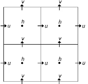
Fig. 1. Finite-difference staggered grids in the ice sheet-shelf model.
hdenotes the centers of h-grid boxes, where ice thickness, ice tem-peratures, and bedrock elevations are calculated.uandvdenote the staggered grid points where horizontal velocity components are cal-culated.
ui(x, y, z)andvi(x, y, z)are ∂ui
∂z = 2A
h
σxz2 +σyz2 +σxx2 +σyy2 +σxy2 +σxxσyy in−21
σxz (1a)
∂vi
∂z = 2A
h
σxz2 +σyz2 +σxx2 +σyy2 +σxy2 +σxxσyy in−21
σyz (1b)
whereσijare deviatoric stresses given below (Cuffey and Pa-terson, 2010). The SSA-like horizontal stretching equations foru(x, y)¯ andv(x, y)¯ are
∂ ∂x
2µh A1/n
(2∂u¯
∂x+ ∂v¯ ∂y)
+ ∂
∂y µ h
A1/n (∂u¯
∂y+ ∂v¯ ∂x)
(2a)
= ρigh
∂hs
∂x + fg
C01/m|ub 2+v2
b|
1−m
2m ub
∂ ∂y
2µh A1/n
(2∂v¯
∂y+ ∂u¯ ∂x)
+ ∂
∂x µ h
A1/n (∂u¯
∂y+ ∂v¯ ∂x)
(2b)
= ρigh
∂hs
∂y + fg
C01/m|u 2 b+v2b|
1−m
2m vb
.
Equation (2a, b) and their horizontal boundary conditions for unconfined ice shelves are derived for instance in Mor-land (1982) and MacAyeal (1996). In Eqs. (2a, b), ub=
¯
u− ¯ui andvb= ¯v− ¯vi whereu¯i andv¯i are obtained from vertical integrations of (1a, b) (e.g., Ritz et al., 1997).
In the zero-order shallow ice approximation, the verti-cal shear stress (σxz, σyz) in Eqs. (1a, b) would be bal-anced only by the hydrostatic driving force −ρig(hs−z) (∂hs/∂x, ∂hs/∂y) acting on the ice column above level z. Here, horizontal stretching forces are included in this force balance (Hubbard, 1999, 2006; Marshall et al., 2005), so that
σxz= −
ρigh
∂hs
∂x − LHSx
hs−z
h
,
σyz= −
ρigh
∂hs
∂y − LHSy
hs−z
h
(3)
where LHSx and LHSy are the left-hand sides of Eqs. (2a) and (2b), respectively. Because horizontal stretching forces are taken to be vertically uniform and the terms in Eq. (2) are forces on the entire ice thickness, their effect on the ice column above levelzis scaled by (hs−z)/hin Eq. (3).
Inclusion of the strain softening terms in Eqs. (1) and (2) due to each other’s flow (i.e.,σxx,σyy,σxyin Eq. (1),∂ui/∂z and∂vi/∂zinµin Eq. (2)), requires manipulation of the con-stitutive relation for ice rheology. In Eq. (2),
µ ≡ 1
2 (ε˙
2)12−nn, (4)
and A = ∫ A dz/h is the vertical mean of the Arrhenius temperature-dependent coefficient in the constitutive relation
˙
εij =A(T )
σ2
n−21
σijor equivalentlyε˙ij=A(T ) 1
n(ε˙2)n2−n1σij (5)
where ε˙ij are strain rates, σij are deviatoric stresses, and ˙
ε and σ are the second invariants of their respective ten-sors. The latter are defined by ε˙2≡ P
ij 1
2ε˙ijε˙ij and σ 2≡
P
ij 1
2σijσij. The relationship
˙ ε2 ≈
∂u¯ ∂x
2 +
∂v¯ ∂y
2 + ∂u¯
∂x ∂v¯
∂y (6)
+1 4
∂u¯ ∂x+
∂v¯ ∂y 2 + 1 4 ∂ui ∂z !2 + 1 4 ∂vi ∂z !2
is used to setµin Eq. (2), and follows using ˙
ε2= ˙ε2xx+ ˙ε2xx+ ˙εxxε˙yy+ ˙εxy2 + ˙ε2xz+ ˙ε2yz,
˙
εxx+ ˙εyy+ ˙εzz=0, ˙
εxx=
∂u¯
∂x, ε˙yy= ∂v¯
∂y, ε˙xy=
1 2
∂u¯ ∂y +
∂v¯ ∂x
,
˙ εxz≈
1 2
∂ui
∂z, ε˙yz ≈
1 2
∂vi
∂z.
The corresponding expression forσ2is used in Eq. (1), and the purely horizontal components are obtained in our numer-ical procedure from
σxx2 +σyy2 +σxy2 +σxxσyy (7)
=
2µ
A1/n
2 "
∂u¯
∂x
2
+
∂v¯
∂y
2
+ ∂u¯
∂x ∂v¯
∂y+ 1 4
∂u¯
∂x+ ∂v¯
∂y
2#
.
The basal sliding relation used on the right-hand sides of Eqs. (2a) and (2b) for grounded ice isu˜b=C0|τb|m−1τ˜b(see Sect. 2.4), or equivalentlyτ˜b=C0−
1
m|ub|
1−m
= 0 andhs=S+h(1−ρi/ρw). (Shere is sea level, andhbis bed elevation).
At each time step, an outer iteration is performed that solves for SSA and SIA velocities, updates ice thicknesses for half of the time step, and re-solves the velocities using the new ice thicknesses, i.e., a second-order Runge-Kutta method. In the solution of Eq. (2) for SSA velocities, a stan-dard (Picard) inner iteration is performed to account for the non-linear dependence ofµand basal sliding on the veloc-ities in Eqs. (2), (4) and (6). The outer iteration converges naturally to the appropriate scaling of SSA vs. SIA flow, de-pending on the magnitude of the basal sliding coefficient. Usually the flow is either almost all vertical shear, with basal drag balancing the driving stress and with negligible stretch-ing, or is almost all longitudinal stretching which balances the driving stress, with small or no basal drag and negligi-ble internal shear. For a fairly narrow range of sliding coeffi-cients, significant amounts of both flow types co-exist.
In each pass of the outer iteration, the SSA Eqs. (2a, b) are solved first, using a sparse matrix method, or optionally, successive over-relaxation (SOR) (or a tridiagonal matrix so-lution for 1-D flow-line problems). Then the ice-thickness advection equation (Sect. 2.6) is time-stepped accounting for both SSA and SIA flow. Ice advection due to SIA is per-formed time implicitly, with the vertically averaged SIA flow given from Eqs. (1) and (3) and using time-implicit linearized Newton-Raphson contributions from allhand∂hs/∂xterms (as in earlier SIA-only model versions; DeConto and Pollard, 2003). Centered ice thicknesses are used for the SIA advec-tion, whereas the time-explicit SSA advection uses upstream ice thicknesses for stability (in Eq. 14 below). An Alternating Direction Implicit (ADI) scheme is used for x vs. y directions (Mahaffy, 1976). A CFL-based maximum speed limit on hor-izontal velocities can be imposed for stability. No ice advec-tion is allowed out of grid cells with sub-grid areal fracadvec-tion
fe<1 (which occurs only for cells at the edge of floating ice shelves, see Sect. 2.9).
CPU time in the model is dominated by the Sparse-Matrix (or SOR) solutions of the SSA equations. As de-scribed in PD09, a considerable reduction in CPU time can be achieved by restricting the full SSA+SIA iterative pro-cedure to grid points with mid-to-high values of the basal sliding coefficient, C(x,y) ≥ 10−8m a−1Pa−2 (see PD12). This range includes all fast streaming regions underlain with deformable sediment (∼10−5). For lower C(x, y) values
<10−8 (including hard bedrock, ∼10−10), the full proce-dure yields virtually 100 % shearing (SIA) flow anyway. At the latter points, advection by internal shear deformation
(u¯i,v¯i), and basal sliding (ub, vb ) are both modeled by standard SIA dynamics. At full SSA+SIA points with C(x,y) ≥ 10−8, advection by internal shear deformation, basal and horizontal stretching are all included in the coupled solution of Eqs. (1) and (2). Tests show that results are essentially unchanged from those with the full SSA+SIA iteration per-formed at all locations.
In intermediate model versions, some simplifications were tried in the coupling dynamics such as neglecting the strain softening cross-terms in Eqs. (1) and (6), which reduced CPU time modestly with only slight effects on the results. Some of these simplifications were used for the figures shown below; however, the most complete and current model version is de-scribed above.
2.3 Grounding-line flux condition
Flow-line tests with hybrid or higher-order models show that in order to capture grounding-line migration accurately, it is necessary either to resolve the grounding-zone boundary layer at very fine resolution (Schoof, 2007; Gladstone et al., 2010a, 2012a; Pattyn et al., 2012a), or to apply an analytic constraint on the flux across the grounding line. The latter approach is used here, with fluxqgacross model grounding lines parameterized as in Schoof (2007, his Eq. 29):
qg = ¯
A(ρig)n+1(1−ρi/ρw)n 4nC
s
!ms1+1 τ xx
τf msn+1
h
ms+n+3
ms+1 g
. (8)
This yields the vertically averaged velocity ug=qg/hg wherehgis the ice thickness at the grounding line. The mid-dle term in Eq. (8) accounts for back stress at the grounding line due to buttressing by downstream islands, pinning points or side-shear, whereτxxis the longitudinal stress just down-stream of the grounding line, calculated from the viscosity and strains in a preliminary SSA solution with no Schoof constraints. The free stress τf is the same quantity in the absence of any buttressing, given by 0.5ρighg (1−ρi/ρw) (cf. Goldberg et al., 2009; Gagliardini et al., 2010).A¯ is the depth-averaged ice rheological coefficient andnis the Glen-Law exponent,Cs is Schoof’s (2007) basal sliding coeffi-cient andms the basal sliding exponent, corresponding here toC−1/m and 1/m, due to the reversed form of the basal sliding law.ρiandρw are densities of ice and ocean water respectively, andgis the gravitational acceleration.hgis in-terpolated in space by first estimating the sub-grid position of the grounding line between the two surrounding floating and grounded h-grid points. This is done by linearly interpolating height above flotation between those two points to where it is zero, linearly interpolating bedrock elevation to that location, and then simply computing the flotation thickness of ice for that bedrock elevation and current sea level (equivalent to LI in Gladstone et al., 2010b).
D. Pollard and R. M. DeConto: Description of a hybrid ice sheet-shelf model 1279
staggered C-grid (Sect. 2.7), where the grounding line is a continuous series of perpendicular segments of u-direction or v-direction interfaces between h-grid boxes, andug (vg) velocities flow across interfaces running through u-grid (v-grid) points. Equations (8–9) and the discussion in this sec-tion applies equally to the y direcsec-tion, withvg andτyy in-stead ofug andτxx. Note that spatial gradients of quanti-ties parallel to the grounding line, which are not included in Schoof’s (2007) flow-line derivation of Eq. (8), are ne-glected here (Katz and Worster, 2010; Gudmundsson et al., 2012; Pattyn et al., 2012b).
We have tested this method of solution in many idealized 1-D flow-line tests, similar to those in Schoof (2007). Our goal was to achieve the same grounding-migration results us-ing a coarse grid (∼10 to 40 km) with those using very fine-grids (∼0.1 km). For coarse grids, we find that it is necessary to impose Eq. (8) as a grounding-line boundary condition. Also for coarse grids we find that an additional rule is nec-essary, because the outer-solution structure of the grounding zone is not fully captured by the grid:
11 grounding line between the two surrounding floating and grounded h-grid points. This is done 1
by linearly interpolating height-above-flotation between those two points to where it is zero, 2
linearly interpolating bedrock elevation to that location, and then simply computing the 3
flotation thickness of ice for that bedrock elevation and current sea level (equivalent to LI in 4
Gladstone et al., 2010b). 5
6
The velocity ug is calculated at the grounding-line points on the u-grid, i.e., those with 7
floating ice in one adjacent (left or right) h-grid box and grounded ice in the other (and 8
similarly for vg on the v-grid). These velocities are imposed as an internal boundary condition 9
for the flow equations, in effect overriding the large-scale velocity solution at the grounding 10
line. This procedure only considers one-dimensional dynamics perpendicular to the grounding 11
line, as in the 1-D flowline analysis in Schoof (2007). It works naturally with the staggered C-12
grid (section 2.7), where the grounding “line” is a continuous series of perpendicular 13
segments of u-direction or v-direction interfaces between h-grid boxes, and ug (vg) velocities 14
flow across interfaces running through u-grid (v-grid) points. Eqs. (8-9) and the discussion in 15
this section applies equally to the y direction, with vg and τyy instead of ug and τxx. Note that 16
spatial gradients of quantities parallel to the grounding line, which are not included in Schoof 17
(2007)’s flowline derivation of Eq. (8), are neglected here (Katz and Worster, 2010; 18
Gudmundsson et al., 2012; Pattyn et al., 2012b). 19
20
We have tested this method of solution in many idealized 1-D flowline tests, similar to those 21
in Schoof (2007). Our goal was to achieve the same grounding-migration results using a 22
coarse grid (~10 to 40 km) with those using very fine-grids (~0.1 km). For coarse grids, we 23
find that it is necessary to impose (8) as a grounding-line boundary condition. Also for coarse 24
grids we find that an additional rule is necessary, because the outer-solution structure of the 25
grounding zone is not fully captured by the grid: 26
27
28
29
30
If the flux qg from Eq. (8) is greater than the large-scale shelf-equation’s
flux qm at the grounding line, then ug (= qg/hg) is imposed exactly at the
u-grid grounding-line point; conversely if qg < qm, then ug is imposed one
u-grid box downstream of the grounding-line point. The former is
usually associated with grounding-line retreat, and the latter usually with
grounding-line advance.
(9)
(9)
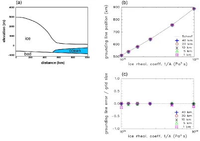
When converting the grounding-line fluxqgfrom Eq. (8) to a velocity (ug), it is important to divide by the ice thickness (calledhgabove) that will effectively be used at the relevant point in Eq. (9) in the finite-difference numerics of the ice advection equation. Then the model’s flux at that point will be exactly that from Eq. (8). In simple equilibrated flow-line tests, this means that the model flux equals the net surface mass balance upstream from the grounding line, an important property of analytic solutions. This yields good agreement with analytic solutions including hysteresis in MISMIP-like tests, using grid sizes of∼5 to several 10s km (Pollard and DeConto, 2011; Docquier et al., 2011; Pattyn et al., 2012a). The agreement can be made almost exact by adjusting the fluxqg for the increment in surface mass balance between the actual grounding line and the point where Eq. (9) is ap-plied, as illustrated in Fig. 2. The analytic solutions in turn agree well with full-Stokes model results, at least in steady-state non-transient situations (Drouet et al., 2011; Pattyn et al., 2012a).
In efforts to minimize single-cell dithering in some ide-alized tests, i.e., flipping back and forth between upstream and downstream points in Eq. (9), two further measures were taken:
i. An initial SSA solution is done at each time step, with-out any imposed flux from Eq. (8), to calculate the
large-scale flux that is compared to the imposed flux in Eq. (9). Previously the large-scale flux was estimated by local finite differences.
ii. Values of the imposed velocities from Eq. (8) are cal-culated for both upstream and downstream points of the grounding line, and these are imposed in the flow equa-tions with weights between 0 and 1 depending on how much (and with what sign) the large-scale flux differs from the imposed flux as in Eq. (8).
These measures had little effect on the dithering in flow-line tests, but fortunately no associated degradation of large-scale results has been detected.
2.4 Basal sliding coefficients
Basal sliding is treated similarly to PD09 by a standard drag law (Cuffey and Paterson, 2010; Pattyn, 2010; Le Brocq et al., 2011)
˜
ub = C0 |τb|m−1τ˜b (10)
where u˜b is basal sliding velocity, τ˜b is basal stress, and m=2 as in Sect. 2.2. As described in PD12, the sliding co-efficientC’ depends on homologous basal temperature, im-plicitly representing basal hydrology:
C0 = (1−r) Cfroz +r C(x, y) (11)
wherer= max0,min1, (Tb+3)3
where C(x, y) is the full sliding coefficient, and Cfroz = 10−20ma−1Pa−2(which is small enough to prevent any dis-cernible sliding, but is not exactly zero to avoid divide-by-zero exceptions in the numerics). Tb (◦C) is the homolo-gous basal temperature, i.e., relative to the pressure melt pointTm= −.000866hwherehis ice thickness (m). There is no sliding below the threshold homologous temperature (−3◦C), ramping up linearly to full sliding at the melt point.
C(x, y) is a specified basal sliding coefficient repre-senting intrinsic bed properties. In PD09 it was two-valued, depending on whether the modern rebounded Antarctic bedrock is above or below sea level: if above,C(x, y)=10−10m a−1Pa−2representing hard bedrock (mainly EAIS), and if below, C(x, y)= 10−6m a−1Pa−2 representing deformable sediment (mainly WAIS) (e.g., Studinger et al., 2001) shown in Fig. 3a. In PD12, a sim-ple inverse method is used that attempts to deduce the real distribution ofC(x, y)under modern Antarctica, constrained to the range 10−10to 10−5m a−1Pa−2.
Fig. 2. Idealized flow-line model tests, similar to basic MISMIP (Pattyn et al., 2012), with uniform surface mass balance, an ice divide
at the left-hand boundary, a forward-sloping bed into ocean, and using surface-mass-balance increments toqg (see text). (a) Geometry
showing sloping bed and ice sheet profiles. (b) Model equilibrated grounding-line positions vs. 1/rheological coefficientA, for various grid sizes and initial states. Solid line shows the analytic solution (Schoof, 2007). (c) As (b) except showing model error (model minus analytic grounding-line position), divided by grid size.
Fig. 3. Basal sliding coefficients C(x, y). (a) Simple two-valued map: blue=10−10m a−1Pa−2 (hard bedrock) where modern ice-free rebounded modern bed is above sea level, orange=10−6m a−1Pa−2 (deformable sediment) where below (PD09). (b) Deduced from inverse-method fitting to modern ice sur-face elevations (PD12, with basal temperature and bedrock relief affecting sliding), 20 km resolution.
We attempt to parameterize this sub-grid process by modi-fying the width of the basal-temperature ramp in Eq. (11), replacing it by
C0 = (1−r) Cfroz + r C(x, y) (12a)
wherer= max0,min1, (Tb−Tr)
(−Tr)
and
Tr = −3 − 500 max [SA−.02,0] − .05 maxheqb −1700,0
(12b)
where SA is the mean sub-grid slope amplitude computed by averaging the bed slopes in the 5-km ALBMAP dataset (Le Brocq et al., 2010) within each model grid box. This quantity was also used by Marshall et al. (1996) in another context.heqb is the ice-free, isostatically rebounded, 9-point-smoothed bed elevation on the model grid, used to mimic SA in data-sparse regions (PD12). The values of the constants are discussed in PD12. Whitehouse et al. (2012) apply a sim-ilar increase in sliding coefficient over mountainous terrain, for much the same reasons. Equation (12) and the associated inverse-derivedC(x, y)distribution (Fig. 3b) are used in the simulations below.
For grid points where the full SSA+SIA iteration is per-formed (Sect. 2.2), C0 andub enter in the right-hand side of the SSA in Eq. (2), where Eq. (10) is inverted to give
D. Pollard and R. M. DeConto: Description of a hybrid ice sheet-shelf model 1281
Fig. 4. (a) Sectors used in sub-ice oceanic melt parameterization. Yellow: Amundsen and Bellingshausen Seas, and western
Penin-sula. Blue: Weddell embayment. Purple: East Antarctica. Red: Ross embayment. (b) Sub-ice oceanic melt rates (m a−1)in modern simulation with 20 km resolution. The average values for each ma-jor shelf are reasonable (Nicholls et al., 2009; Olbers and Hellmer, 2010; Dinniman et al., 2011), although somewhat lower for the Ross. Rates are noticeably larger nearer the grounding lines due to the depth dependence of the freezing pointTfin Eq. (17), especially
in Pine Island and Prydz Bays, but not noticeably for the flatter Ross Ice Shelf.
contributions from Eq. (10) in the same way as for internal shearing in Eq. (1).
2.5 Sub-grid pinning points
Under the major ice shelves, there may be sub-grid pinning points due to small bathymetric rises scraping the bottom of the ice, especially near the grounding line, that are un-resolved by the model grid. This is parameterized simply in terms of the standard deviation of observed bathymetry within each model cell. The fractional areafgof ice in con-tact with sub-grid bathymetric high spots is
fg = 0.5 max
0, 1 − hw sdev
(13) wherehw is the thickness of the ocean column between the cell-mean bedrock and ice base, andsdevis the standard de-viation of the observed bed elevations (ALBMAP, 5 km, Le Brocq et al., 2010) within the cell. For 20 to 40 km grids,sdev is typically smaller than∼50 m under the Ross and much of the Weddell and Amery ice shelves, but up to to a few 100s m in isolated patches of the Weddell, Lambert, and much of Pine Island Bay.
fghere is identical to thefgin Eqs. (2a, b), and modifies the basal stress for the cell. Instead of no drag (fg= 0, freely floating ice), the value from Eq. (13) is used, increasing the basal stress tofgtimes the amount for 100 % basal contact.
In effect, this augments the overall drag on the ice shelf in addition to side drag, which is transmitted upstream within the SSA equations, increasing buttressing and reducing ice flux across the grounding line, i.e., makingτxx less positive and reducingqg in Eq. (8). The extent and importance of small-scale pinning is somewhat speculative, and deserves more study, observationally by examination of surface
fea-tures or improved bathymetry (Horgan and Anandakrishnan, 2006; Fricker et al., 2009; Hulbe et al., 2010; Timmermann et al., 2010), and by modeling such as Favier et al. (2012).
2.6 Ice thickness
∂h
∂t = −
∂(uh)¯
∂x −
∂(vh)¯
∂y (14)
+ SMB − BMB − OMB − CMB − FMB
where SMB=surface mass balance, BMB=basal melting (if grounded), OMB=oceanic sub-ice melting or freez-ing (if floatfreez-ing), CMB=calving loss (floating edge), and FMB=face melt loss (floating or tidewater vertical face).
The time stepping of the ice thickness equation is done as part of the iterative solution of ice velocities as described in Sect. 2.2. The treatments of the various local ice gains or losses (SMB, etc) are described in later sections.
2.7 Ice temperature and rheology
The prognostic equation for internal ice temperatures
T (x, y, z0, t )is
∂T ∂t = −u
∂T ∂x −v
∂T ∂y − w
0∂T
∂z0 (15)
+ 1
ρicih2
∂ ∂z0
ki
∂T ∂z0
+ Qi
ρici
wherez0=(hs−z)/ h,ki = 2.1×365×86 400 J a−1m−1 K−1 is ice thermal conductivity, and Qi is internal shear heating due to both SIA and SSA deformation. Only ver-tical heat diffusion is included; horizontal heat diffusion is assumed negligible on scaling grounds. Note that the ver-tical coordinate z0 is dimensionless, and Eq. (15) has been transformed to this coordinate system (Huybrechts and Oer-lemans, 1988; Ritz et al., 1997). The transformed verti-cal velocityw0=dz0/dt; numerical calculation of w0 uses the technique in Ritz et al. (1997) (whose wt is our w0h). Horizontal velocities u, v are the sum of internal (∼SIA) shear and the basal velocity. The large-scale advective terms (−u∂T/∂x – v∂T/∂y – w0∂T/∂z0) are calculated time-explicitly, using upstream parabolic interpolation forT (Far-row and Stevens, 1995).
The upper boundary condition is T(x,y,0,t)= surface ice temperature, deduced from surface air temperatures (Sect. 3). For grounded ice, the lower boundary condition at the ice base is that the vertical conductive flux (ki/ h) ∂T/∂z0 at z0=1 is equal to the vertical conductive flux at the top of
the bedrock (see below) plus any basal shear heatingQb= ˜
Equation (15) is time-stepped with the vertical diffusive terms and boundary conditions treated time implicitly, which involves a standard tridiagonal solution versusz0for each ice column. To avoid numerical instability, very small ice thick-nesses (<1 m) are treated as a thin film with zero heat ca-pacity, but still with latent heat and melting if its temperature would otherwise exceed the pressure melt point.
Surface melting, refreezing and locally mobile liquid are calculated along with the surface mass balance (Sect. 3). Any locally mobile liquid (rain, snow melt and ice melt, minus refreezing) is assumed to immediately percolate downwards into the local vertical ice column, exchanging its latent heat with the sensible heat of the next lowest layer, i.e., if the layer is below freezing, then some (all) of the percolating liquid freezes, raising the layer temperature to (towards) the pres-sure melt point (and adding to the layer thickness). If the melt point is reached, the remaining water percolates down to the next layer, and so on. If any liquid reaches the base, it is added to any ice melt at the base itself, and is simply recorded as mass lost from the model (there is no basal hy-drologic component).
The model includes vertical heat diffusion and storage in bedrock below the ice, heated from below by a speci-fied geothermal heat flux. Nominally, and in all simulations shown below, its effect is minimized by using a very thin (30 m) single layer, so that the geothermal heat flux is essen-tially applied to the base of the ice. In other applications, it is typically∼2 km thick with 6 unequally spaced layers (cf. Ritz et al., 1997). Physical and thermal properties of bedrock are given in Table 1.
In the ice dynamics (Sects. 2.2 and 2.3), the ice rheological coefficientAand its dependence on temperature are specified as in Huybrechts (1998):
A=E×5.47×10¹⁰e−13.9×10⁴/(8.314T0) (16a) ifT0≥263.15◦K
A=E×1.14×10⁻⁵e−6.0×10⁴/(8.314T0) (16b) ifT0<263.15◦K
whereT0is the homologous ice temperatureT −Tm, where Tm= −.000866zis the pressure melting point (◦C) andzis depth (m) below ice surface. Units ofAare a−1Pa−3 corre-sponding ton=3 in Eqs. (1) to (7). The enhancement factor
Eis set to 1 for SIA flow in Eq. (1) (see PD12), and to 0.3 for SSA flow (Eqs. 2 and 8). The ratio of enhancement factors represents differences in fabric anisotropy between grounded and shelf ice (Ma et al., 2010); it is similar to but somewhat smaller than their suggested range of 5:1 to 10:1.
2.8 Sub-ice-shelf oceanic melting
The simulation of oceanic melting at the base of Antarctic ice shelves is challenging, involving incursions of Circumpolar Deep Water (CDW) or High Salinity Shelf Water (HSSW)
and other mechanisms that differ from basin to basin (e.g., Nicholls et al., 2009; Walker et al, 2009; Jenkins et al., 2010; Pritchard et al., 2012). Coupling with ice sheet models will ultimately require high-resolution 3-D regional ocean mod-eling (e.g., Dinniman et al., 2011; Hellmer et al., 2012), espe-cially for paleo and future scenarios. For now, we use simple parameterizations that attempt to provide (i) the basic mod-ern spatial distribution, and (ii) paleoclimatic variations that yield results in accord with geologic data.
In PD09, the parameterization of modern oceanic melt rates was somewhat ad hoc, based on subtended arcs to open ocean. Our current parameterization described below follows Martin et al. (2011) for the PISM-PIK model. A new param-eterization based on Olbers and Hellmer’s (2010) more phys-ical cavity-box model (Gladstone et al., 2012b; Winkelmann et al., 2012) is under development.
Similarly to Martin et al. (2011), the oceanic melt rate at the base of floating ice (m a−1), OMB in Eq. (14), is given by
OMB = K KTρwcw ρiLf
To−Tf
To−Tf (17) whereTo is the specified ocean water temperature, and Tf = .0939 – .057×34.5 – .000764 z(◦C) is the ocean freez-ing point at ice-base depth z (m) (Beckmann and Goose, 2003; cf. Jenkins and Bombosch, 1995). The transfer fac-torKT= 5 ×10−7×365×86 400 = 15.77 m a−1K−1 (as in Martin et al. atTo−Tf= 1◦C), andKis an additionalO(1) basin-dependent factor given below. Because the freezing point Tf decreases with depth, the dependence on To−Tf means that melt rates tend to be higher at the grounding line as deduced from observations. Unlike Martin et al. (2011), the dependence on temperature differenceTo−Tfis quadratic (Holland et al., 2008).
Here, the ocean temperatureTois specified differently for various Antarctic sectors, based on observations but mainly aiming to produce realistic modern ice-shelf extents and grounding-line positions. The 4 sectors are delineated by crude latitude and longitude ranges, as follows (with latitudes in◦N, longitudes in ◦E, temperatures in◦C, and depths in meters), and also shown in Fig. 4a.
– Amundsen and Bellingshausen Seas,
and Western Peninsula:
[longitude, latitude]=[−140 to −120, >−77] or [−120 to−90,>−85] or [−90 to−65,>−75].
To−Tfdepends on depthz, based loosely on profiles in the outer Pine Island Bay with an upper layer of colder fresher water (Jacobs et al., 2011), which may be im-portant for the survival of smaller shelves with shal-low grounding lines:To−Tf=0.5 forz <170, 3.5 for z >680, joined linearly from 170 to 680 m.
D. Pollard and R. M. DeConto: Description of a hybrid ice sheet-shelf model 1283
– Weddell embayment:
[longitude, latitude]=[−120 to−90,<−85] or [−90 to−65,<−75] or [−65 to−10, all].
To= −0.8 K=1
– East Antarctica:
[longitude, latitude]=[−10 to 160, all].
To−Tf and K are as for the Amund-sen/Bellinghausen/W. Peninsula sector, even though ocean profile data in Prydz Bay for instance do not indicate a distinct upper layer as clearly as for Pine Island Bay (Smith et al., 1984).
– Ross embayment:
[longitude, latitude]=[160 to 180, all] or [−180 to −140, all] or [−140 to−120,<−77].
To= −1.5 K=1
At this point,ToandKrepresent conditions under modern exposed shelves. For the West Antarctic sectors, ocean melt is further reduced based on subtended arc to open oceanAa (degrees), i.e., the angle formed by the set of all straight lines from the point in question that reach open ocean without hit-ting land (as in PD09).
To0=Towa + (−1.7) (1−wa) (18a)
K0= K wa + 1×(1−wa) (18b)
where
wa=max[0,min[1, (Aa−50)/20]] (18c) This has the effect of reducing ocean melting for regions mostly surrounded by land. It is found to be necessary in long-term paleo runs (Sect. 5 below) to allow WAIS to re-grow after a collapse of all marine ice. After a collapse, the surviving small terrestrial ice caps on Western Antarctic is-lands must first form thin ice shelves that grow over the inte-rior seaway, coalesce, thicken and become buttressed so as to allow grounding lines to advance out from the islands. Equation (18) can be justified by arguing that interior sea-ways mosly surrounded by land were more protected from warm water intrusions than the modern coast and embay-ments. This hypothesis should be tested by regional ocean modeling of the environment following a major WAIS col-lapse. Equation (18) is not applied to East Antarctica for the ad hoc reason that ocean melting from Eq. (17) needs to pen-etrate into the Lambert Graben in order to produce reason-able modern grounding line and shelf extents there. A simi-lar parameterization to Eq. (18) is also used to restrict calving (Sect. 2.10).
The above yields the distribution of modern ocean melt rates, shown in Fig. 4b. For paleoclimatic applications, long-term climate variations are parameterized much as in PD09, based on a single weighting parameterwcset proportional to deep-sea coreδ18O, plus a slight influence of austral summer insolation:
wc = max
0,min2,1+S/85+1×log(rCO2)/log(2)
+max[0,0.11Q80/3]]] (19) whereSis eustatic sea level relative to modern (meters), set proportional toδ18O (Lisiecki and Raymo, 2005) with mod-ernδ18O corresponding to 0 m and Last Glacial Maximum
δ18O corresponding to−125 m.1Q80is the change in Jan-uary insolation at 80◦S from modern (W m−2)(Laskar et al., 2004). rCO2is atmospheric CO2in units of preindustrial level (280 ppmv), used mainly for deeper time (pre-Pliocene) experiments. For fixed pre-industrial CO2,wcvaries between 0 for glacial maxima, 1 for modern-like climates, and 2 for warmest interglacials.wcis converted to 3 weights for those 3 climates (each between 0 and 1, summing to 1):
wlgm=(1−wc), wmod=wc, whot=0 for 0≤wc≤1 (20a) wlgm=0, wmod=(2−wc), whot=(wc−1)for 1< wc≤2 (20b) which are used to alter the ocean temperature and basin factor from Eq. (18):
To00 = −1.7wlg m+T
0
owmod + 5whot (21a)
K00 =K0wlg m+K
0
wmod+8whot (21b)
Finally,To00andK00are modified for distal locations, to pre-vent ice shelves from expanding into the Southern oceans far from Antarctica. This is based on ocean bathymetry (hw = sea level –hb), assuming much warmer waters at depths >∼2000 m, with an additional constraint based on the arc-to-open-ocean angleAa to ensure this is not done for deep proximal troughs. The finalTo000andK000are used in Eq. (17) in place ofToandK.
To000 = To00(1−wdwe)+ max[T
00
o, Tdist]wdwe (22a)
K000=K00(1−wdwe) +10wdwe (22b) where
Tdist= −0.5wlgm+5wmod+8whot (22c)
wd=max[0,min[1, (hw−1900)/200]] (22d)
2.9 Sub-grid ice shelf fraction
In order for the model to represent vertical tidewater faces, and to avoid whole grid-cell jumps in the advance and retreat of ice shelves, floating ice is allowed to occupy a subgrid fraction of cell area,fe. This is only applied at ice shelf edges adjacent to open ocean; for interior shelf and all grounded points,fe = 1. The motivation and method here closely fol-low Albrecht et al. (2011) for the PISM-PIK model.
For floating ice cells adjacent to open ocean, the sub-grid actual thickness (within the areafe)is estimated based on the thickness of adjacent, presumably upstream, ice (Albrecht et al., 2011). All adjacent points are examined, and the max-imum of their ice thicknesses (h)is taken, but only if they are grounded, or are floating and not themselves adjacent to open ocean. Furthermore, if grounded, the interpolated thick-ness at the grounding line is used.
Then this maximum thickness,hmax(m) say, is reduced to allow for typical downstream thinning into the cell in ques-tion:
he =max h
hmaxmax(0.25, e(−hmax/100)), 30, h i
(23) where the minimum of 30 m avoids very thin shelves, andhe can also not be less than the current cell-mean thicknessh.
heis the estimated actual ice thickness within areal fraction feof the cell in question.
Finally, to implicitly conserve ice mass, the fractional area occupied by ice in this cell is reset to
fe=h/ he (24)
wherehis the cell-mean thicknessh(ice volume divided by cell area). Note that the settings above are only done for float-ing ice cells adjacent to open ocean, otherwisefe = 1 and he=h. The variable fe is used elsewhere in the model to scale quantities that truly depend on area of ice, i.e., surface mass balance and oceanic melting are both multiplied byfe in the ice thickness evolution as in Eq. (14). Also, as men-tioned in Sect. 2.2, no advective flow of ice is allowed out of a cell withfe<1.
2.10 Calving at ice-shelf edge
There has been considerable recent activity in modeling calv-ing of tidewater glaciers and ice shelves, in part because the extent of floating ice can affect the amount of back stress (buttressing) at the grounding line, and hence the stability of grounded ice upstream (Scambos et al., 2004). Various mech-anisms or triggers have been represented in models, includ-ing ice thickness over flotation, penetration of crevasses and surface water, and large-scale stress fields (reviewed by Benn et al., 2007; also for instance Alley et al., 2008; Nick et al., 2010; Levermann et al., 2012), but there is little consensus on the main mechanism or mechanisms.
The calving parameterization here is based on the large-scale stress field, represented by the horizontal divergence of
Fig. 5. (a) Divergence∂u/∂x+∂v/∂y(a−1) of floating ice, in nested 10 km modern simulation with constrained grounding lines and shelf geometry (as in PD12). (b) Loss due to calving (CMB, m a−1).
floating ice velocities. It shares the same motivation as earlier studies by Doake et al. (1998) and is similar to the parame-terization in PISM-PIK (Martin et al., 2011; Winkelmann et al., 2011; Levermann et al., 2012), but without using princi-pal strains, i.e., with no distinction between along-flow and across-flow strains, as in Amundson and Truffer (2010). In-clusion of fracture propagation (e.g., Hulbe et al., 2010; Al-brecht and Levermann, 2012), multiple stable states (Lever-mann et al., 2012) and other calving mechanisms are deferred to future work.
First, the divergence of floating ice shelf points div is cal-culated as
div=∂u/∂x¯ +∂v/∂y¯ (25)
usingu¯andv¯from the solution of the SSA Eqs. (2a, b) above. This is done only for floating grid points with full fractional cover (fe=1, Sect. 2.9), and propagated by nearest-neighbor value to those on the shelf edge withfe<1. Then, for points at the shelf edge adjacent to open ocean, the grid-mean calv-ing loss CMB (m a−1, used in Eq. 14) is set as a weight be-tween two values:
CMB = (1−wc)30 + wc3×105max(div,0) he/dx (26) where the weightwc= min (1,he/200). Here,heis the sub-grid thickness of ice within fraction fe (Sect. 2.9), and dx is the grid cell size. All units are meters and years. For thin shelves (he<<200 m), calving is simply weighted towards a constant value of 30 m a−1. For thicker shelves, it is weighted towards a value proportional to divergence div (a−1), but only for positive div.
The thicknessheand grid size dx enter in Eq. (26) because 3×10⁵max (div, 0) represents the calving rate (i.e., average horizontal speed of erosion of the shelf edge into the interior,
Uc in Benn et al., 2007), but CMB here is the rate of vol-ume of ice removed from the cell divided by cell area, so the expression is multiplied byhedx/dx2.
D. Pollard and R. M. DeConto: Description of a hybrid ice sheet-shelf model 1285
West Antarctic shelves, ice velocities change significantly upstream on scales of several 100s km, LT say, so the di-vergence at the edge is on the order ofUT divided byLT. In that case, the parameterizedUc= 3×10⁵UT /LT, which is the same order asUT as required for steady state.
CMB is further modified for seaways mostly surrounded by land, represented by the angle subtended to open ocean,
Aa. This quantity is also used to modify oceanic melt (Sect. 2.8, Eq. 18). As discussed in that section, these modifi-cations are needed to allow regrowth of thin shelves in central West Antarctic seaways following a major WAIS collapse (in contrast to the vigorous calving at the edges of the thicker Ross and Weddell shelves today). It can be motivated by con-sidering the effects of icebergs clogging in the restricted sea-ways, possibly creating a melange that inhibits further calv-ing, but this needs to be explored by future modeling (cf. Vaughan et al., 2011). The calving loss rate CMB is reduced by
CMB0 = CMB max
0,min
1, (Aa−70)20 (27) The divergence div and calving loss given by Eqs. (26) and (27) are shown in Fig. 5 for a modern nested West Antarctic simulation. In practice, ice-edge thicknesses are often con-siderably less than 200 m, so the weightwcin Eq. (26) is∼0, and CMB is close to the constant 30 m a−1in many regions, as seen in Fig. 5. This will be improved in a new calving parameterization under development (see below).
For past climates, calving is reduced for cooler environ-ments, similarly to ocean melt in Sect. 2.8. This is some-what ad hoc, because the dependence of divergence on calv-ing does not directly depend on temperature, as some of the other mechanisms mentioned above. But we find that calving must be reduced in order to allow grounding lines to expand as observed during glacial maximum periods.
CMB00 = CMB0(0×wlgm+1×wmod + 1 ×whot) (28) wherewlgm,wmod andwhot are the 3 climate weights cor-responding to glacial maxima, modern-like and warm inter-glacial conditions (as in Sect. 2.8, Eq. 20). We are currently developing a new calving parameterization with surface melt dependence, which may avoid the questionable dependencies in Eqs. (27) and (28).
2.11 Oceanic melt at vertical faces
The parameterization of sub-grid areal fraction in Sect. 2.9 allows tall vertical ice faces to be in contact with the ocean, including tidewater fronts extending one grid cell from deep grounding lines. Observations at Greenland calving faces show that oceanic melting of the submerged ice front can be up to a few meters per day (Rignot et al., 2010). A parame-terization of the actual circulation and melt rates at a vertical face (Motyka et al., 2003) is not yet in the model. As a place-holder for now, we calculate the area of each vertical face
in contact with the ocean, and simply apply oceanic sub-ice melt rates from Sect. 2.8 to that area. For any ice cell adja-cent to and in contact with open ocean, the vertical extent of submerged ice is
1z = ρi ρw
hefor floating ice (29a)
1z = S −hbfor grounded ice (29b)
whereSis sea level andhbis bed elevation. For each of the (up to 4) neighboring cells with no ice and open ocean,1z is multiplied by the length of the interface (dx for Cartesian grids) and by that cell’s oceanic sub-ice melt (OMB from Sect. 2.8). These are summed, and divided by the cell area (dx2)to yield the cell-mean loss of ice due to face melting FMB used in Eq. (14).
2.12 Bedrock deformation
As in Huybrechts and de Wolde (1999) and Ritz et al. (1997, 2001), the response of the bedrock to the changing ice and ocean load is a combination of time-lagged asthenospheric relaxation towards isostatic equilibrium, and modification of the applied load by the elastic lithosphere. The treatment here exactly follows Huybrechts and de Wolde (1999). The down-ward deflection wb of the fully relaxed response (as if the asthenosphere had no lag) is given by
D∇4wb + ρbgwb = q (30)
whereD= 1025N m is the flexural rigidity of the lithosphere,
ρbis the bedrock (asthenospheric) density andgis gravita-tional acceleration. A lower value ofD(∼1023to 1024N m) can optionally be used for West Antarctica (cf. Stern and ten Brink, 1989). The applied loadqis
q=ρigh+ρwghw−ρigheqi −ρwgheqw (31) wherehis ice thickness,hwis ocean column thickness, and heqandheqw are their values in the equilibrium state (see be-low).
Equation (30) is solved by a Green’s function method. The response to a point loadP (q times area) versus radial dis-tanceris
wp(r) =
P L2
2π D kei r
L (32)
load alone (Brotchie and Silvester, 1969). The actual bedrock rate of change is given by
∂hb
∂t = −
1
τ hb −h eq b +wb
(33)
wherehbis current bedrock elevation,heqb is its equilibrium value, andτ is 3000 yr.
The equilibrium state (heqandheqw in Eq. 31,h eq
b in Eq. 33) is taken to be the modern observed, assuming that any glacial isostatic adjustments still to occur from the last deglaciation can be neglected (cf. PD12 Appendix B). Equivalently, at the start of a run, the bedrock model alone can be spun up for several 10 000s years with all ice removed, and the resulting ice-free equilibrated state can be used to defineheqb ,heqw (and heq= 0).
2.13 Time steps, adaptive time stepping
The main ice-dynamical time step 1ti (for Eq. 14) is se-lected for most experiments depending on model resolution, for instance∼0.1 to 0.5 yr for 5 to 10 km,∼0.5 to 1 yr for 20 km, and 2 to 5 yr for 40 km. There is an option for adap-tive time stepping that circumvents numerical instabilities, as follows. A restart file is saved at regular time points dur-ing a run (spaced∼1000 yr apart typically). If a numerical exception (NaN) occurs or if physically unreasonable val-ues of ice thickness, temperature or velocity are detected, the simulation reverts to the previous time point using the last restart file, and tries again to run through the next 1000 yr with the time step halved. If an anomaly still occurs during the next 1000 yr, the process is repeated, and is attempted up to 4 times (i.e., with time steps as small as 2−4×the nomi-nal value) before aborting. If an attempt makes it through the next 1000 yr successfully, the time step is reset to the nominal value and the run continues on.
For the NetCDF history files, no special action is needed if this adaptive time-looping occurs, because the model snap-shots have a unique time index and overwrite any previous snapshot with the same time value. For sequential (ascii) files that contain output at regular intervals, marker records are written that allow a postprocessing program to recognize any time-looping and delete repeated sections as needed. The adaptive-time-stepping capability can be convenient near the start of experiments that are initialized to a state far from equilibrium with the boundary conditions (e.g., mod-ern ice sheet and other geologic time periods). In those cases, blowups and adaptive time looping tend to occur in the first few hundred years, after which the model becomes adjusted to the boundary conditions and the run continues normally.
Other components of the model are time-stepped or reset at greater intervals. The various intervals are as follows:
– Ice thickness and dynamics Eq. (14):1ti, depends on resolution as above.
– Ice and bed temperatures Eq. (15): 50 yr, or 1ti for 10 km resolution or less.
– Bedrock deformation Eq. (33): 50 yr.
– Resetting oceanic melt and calving parameterizations
(Sect. 2.8 and 2.9):1ti.
– Resetting parameterized climate (Sect. 3): 50 yr.
– Resetting climate from global or regional climate
mod-els (Sect. 3): 1000 yr.
– Recalculating mass balance on ice surface (Sect. 3): 50
to 100 yr. At intervening times, recalculation is done for any ice points whose elevation changes by more than 50 m.
3 Input datasets and climate forcing
Modern Antarctic input fields are obtained mainly from the ALBMAP v1 dataset at 5 km resolution (Le Brocq et al., 2010). The fields used to determine the equilibrium ice and bedrock state discussed in Sect. 2.12, with ALBMAP names in parentheses, are ice surface elevation (usrf), bedrock to-pography (lsrf, topg), and ice thickness (thk).
Various geothermal heat flux maps can be used in the model (Shapiro and Ritzwoller, 2004 (bheatflx shapiro); Fox Maule et al., 2005 (bheatflx fox); Pollard et al., 2005), but these differ considerably from each other on regional scales with noticeable effects on modern results (see next section). Rather than choose one or the other, in the nominal model we specify a simple two-value pattern, with 54.6 mW m−2 under EAIS and 70 mW m−2under WAIS.
For runs with parameterized climate, observed annual ac-cumulation rateP (van de Berg et al., 2006 (accr)) and sur-face air temperatureTa (Comiso, 2000 (temp)) are used to calculate modern surface mass budgets, as follows:
1. First,Ta andP are horizontally interpolated to the ice model grid, and vertical lapse rate corrections are ap-plied:
Ta0=Ta−γ (hs−hobss ) (34a)
P0=P×2(T
0
a−Ta)
.
1T
(34b) whereγ = .0080◦C m−1,1T is 10◦C (15◦C in some runs),
hs is the model surface elevation and hobss is the modern observed elevation interpolated to the ice grid (similarly to Huybrechts, 1998; Ritz et al., 2001).
D. Pollard and R. M. DeConto: Description of a hybrid ice sheet-shelf model 1287
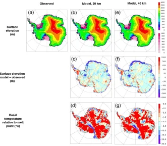
Fig. 6. (a) Left column (a): Modern observed (Le Brocq et al., 2010, averaged to 20 km grid). Middle column (b–d): Model, using
basal sliding coefficient distribution from inverse method described in PD12, 20 km grid. Right column (e–g): Model, 40 km grid. Top
row: Grounded ice surface elevations (upper scale) and floating ice thicknesses (lower scale), meters. Middle row: Difference in surface
elevations, model minus observed, meters. Bottom row: Model basal homologous temperature (relative to pressure melting point),◦C.
3. A basic positive degree -day (PDD) scheme is applied to the monthly cycle, with coefficient .005 m of melt per degree day. Monthly precipitationP0is either rain or snow depending on whether monthly air temper-ature is above or below 0◦C. Any melt or rain im-mediately becomes mobile and percolates into the ice sheet (Sect. 2.7). For modern runs, there is very little surface melt or rain on Antarctic ice. For paleo and fu-ture runs with significant melt and rain, a more detailed PDD scheme is available with seasonal refreezing, snow with liquid storage, distinct snow vs. ice PDD coeffi-cients, and allowance for diurnal and synoptic variabil-ity (cf. Marshall et al., 2004). In future work we plan to include insolation explicitly (van de Berg et al., 2011). 4. The surface ice temperature, needed as a boundary
con-dition in Sect. 2.7, is assumed to be the annual mean of min [monthly air temperature, 0◦C].
For paleoclimate runs with parameterized climate, the modern surface Ta0 and P0 are modified, very much as in PD09:
A. A spatially uniform shift1Tais applied to air temper-atures, mainly determined by deep-sea coreδ18O and
CO2, with a minor effect of austral summer insolation (similarly to past ocean melt variations in Sect. 2.8, Eq. 19):
1Ta = 10S
125 + 10 log(rCO2) log(2) + 0.11Q80 (35)
whereS(meters) is eustatic sea level relative to modern, pro-portional toδ18O (as for Eq. 19). rCO2is atmospheric CO2 in units of preindustrial level (280 ppmv), assumed to pro-duce a 10◦C warming in the Antarctic region for each CO2 doubling.1Q80(W m−2)is the change in January insolation from modern at 80◦S.1Tais applied on the right-hand side of Eq. (34a) and so also affects precipitationP0in Eq. (34b). B. The peak-to-peak amplitude of the sinusoidal seasonal temperature cycle (nominally 20 to 30◦C, step 2 above) is changed by 0.11SQ80, where1SQ80(W m−2) is the change in January minus July insolation from modern at 80◦S.
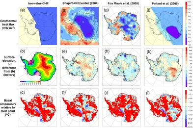
Fig. 7. Modern model results with various prescribed geothermal heat flux (GHF) distributions, 40 km resolution, using basal sliding
coef-ficient distribution from inverse method described in PD12. Left column (a–c): with simple 2-valued GHF, default for this paper. Second
column (d–f): with Shapiro and Ritzwoller (2004) GHF. Third column (g–i): with Fox Maule et al. (2005) GHF. Right column (j–l):
with Pollard et al. (2005) GHF. Top row: GHF distributions, mW m−2. Middle row: (b) Grounded ice surface elevations (upper scale) and floating ice thicknesses (lower scale), meters. (e, h, k): Difference from (b), meters. Bottom row: Basal homologous temperature (relative to pressure melting point),◦C.
above (e.g., DeConto and Pollard, 2003; Koenig et al., 2011; DeConto et al., 2011), or provides its own annual surface mass budgets calculated with full climate-model physics di-rectly to the ice model.
4 Modern results
In this section, some basic model results for present-day Antarctica are compared with observations. These simula-tions have been run to equilibrium with the modern climate, so the comparison ignores any remaining glacial isostatic ad-justments in the real world, which are relatively small com-pared to modern biases (PD12). As discussed in PD12, fur-ther work is planned with transient runs through the last deglaciation and extensive comparisons with paleo data (fol-lowing Briggs et al., 2011; Whitehouse et al., 2012).
Figure 6 compares ice surface elevations hs with ob-served, using the model with parameterized modern cli-mate (Sect. 3) and inverse-derived basal sliding coefficients
C(x, y)(Sect. 2.4; PD12). Due mainly to the inverse-derived
C(x, y), model elevations are within a few 10s meters of ob-served in most regions. Over the Transantarctics and some other mountain ranges, there are small patches with
eleva-tions a few hundred meters too high. As discussed in PD12, these are thought to be due to insufficient sliding through deep troughs cutting through the mountains, only partially compensated by the sub-grid topographic parameterization in Eq. (12); however, further work is needed to test that hy-pothesis.
Much the same level of accuracy inhsis maintained at dif-ferent resolutions (20 km and 40 km in Fig. 6; 10 km nested in PD12), which is somewhat surprising for regions such as the Siple Coast with ice streams that are scarcely resolved at 40 km. Apparently the proto-streaming at 20 and 40 km does capture basic features such as interleaved unfrozen vs. frozen beds (Fig. 6d, g), and provides the correct overall flux to the grounding line. (At 10 km resolution, individual Siple Coast ice streams are simulated quite realistically, including cen-tury time-scale rerouting and stagnating; PD09 Supp. Inf.).
D. Pollard and R. M. DeConto: Description of a hybrid ice sheet-shelf model 1289
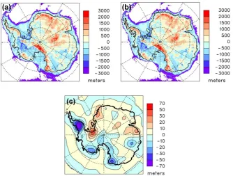
Fig. 8. (a) Bed elevations, meters, in modern simulation at 20 km resolution. (b) Observed modern bed elevations, meters (Le Brocq et al.,
2010). (c) Difference, model minus observed.
lines are reasonably realistic, except that the Ronne ground-ing line has retreated about 200 km too far south (roughly between the Ellsworth Mountains and the Foundation Ice Stream), causing a pronounced low patch in Fig. 6c and f. Other smaller-scale grounding-line errors are seen in Pine Island Bay, Lambert Graben, and especially on the western Peninsula where George VI Sound (between Alexander Is-land and the mainIs-land) is overridden with thick grounded ice in the model. The latter errors may require higher-resolution modeling and/or coupling with ocean models to correct en-tirely, but apart from George VI Sound, the errors are not huge and basic regional features are captured.
Figure 7 examines the model sensitivity to the prescribed geothermal heat flux (GHF) map. As noted above, GHF datasets differ significantly even at large scales (Fig. 7, top row). In PD12 we found that these differences can be accom-modated by small adjustments in the inverse-derived distri-bution of basal sliding coefficientsC(x, y)(see Sect. 2.4). Here, we show the sensitivity of the model with fixedC(x, y)
used in this paper. As shown in Fig. 7, the various GHF maps cause regional and small-scale differences in surface ice elevation of∼100 to 200 m, and significant changes in basal freezing vs. melting patterns. Analogous results are de-scribed in Pattyn et al. (2010) for Antarctica, and Rogozhina et al. (2012) for Greenland.
Modern bedrock elevations are also quite close to ob-served over most regions, showing that the bedrock model in Sect. 2.12 is reasonably realistic (Fig. 8). The largest
dif-ferences are caused by two main grounding-line errors men-tioned above, on the Ronne coast and George VI Sound. However, as discussed in PD12 (Appendices D, E), some of the general agreement may be fortuitous because the model has not taken transient residuals from the last deglaciation into account.
Fig. 9. (a) Observed surface ice velocity (Rignot et al., 2011), averaged here to 20 km model cells, m a−1. (b) Model surface ice velocity, m a−1, in modern simulation at 20 km resolution. (c) Model minus observed log10(velocity, m a−1), i.e., log10(vmodel/vobserved). Very slow
velocities are ignored; i.e., ifvmodelorvobservedis less than 2 m a−1, it is reset to 2 m a−1for this plot. (d) Scatter plot of observed vs. model
velocities (log10(m a−1))for each 20-km grid cell with grounded ice. The same figure appears in PD12.
Fig. 10. Time series of total Antarctic ice volume (106km3)over the last 5 million years, in simulations with parameterized climatic and oceanic forcing dependent mainly on deep-sea coreδ18O, and slightly on austral summer insolation, with 40 km model resolution.
(a) Current model, with inverse-derived basal sliding coefficients
C(x, y), and value on continental shelves=10−5m a−1Pa−2. (b) Earlier model version as in PD09 (their Fig. 3a) with simple two-valuedC(x, y)and continental-shelf value=10−6m a−1Pa−2.
Fig. 11. Grounded ice surface elevations (upper scale, meters)