CH 4parameter estimation in CLM4.5bgc using surrogate global optimization

(1)

www.geosci-model-dev.net/8/3285/2015/ doi:10.5194/gmd-8-3285-2015

CH

4 parameter estimation in CLM4.5bgc using surrogate global

optimization

J. Müller1, R. Paudel2, C. A. Shoemaker3, J. Woodbury3, Y. Wang3, and N. Mahowald2 1_{Center for Computational Sciences and Engineering, Lawrence Berkeley National Laboratory,}

Berkeley, CA 94720, USA

2_{Earth and Atmospheric Sciences, Cornell University, Ithaca, NY 14853, USA}

3_{School of Civil and Environmental Engineering, Cornell University, Ithaca, NY 14853, USA} Correspondence to: J. Müller ([email protected])

Received: 4 November 2014 – Published in Geosci. Model Dev. Discuss.: 6 January 2015 Revised: 24 June 2015 – Accepted: 5 October 2015 – Published: 20 October 2015

Abstract. Over the anthropocene methane has increased

dra-matically. Wetlands are one of the major sources of methane to the atmosphere, but the role of changes in wetland emis-sions is not well understood. The Community Land Model (CLM) of the Community Earth System Models contains a module to estimate methane emissions from natural wetlands and rice paddies. Our comparison of CH4emission

observa-tions at 16 sites around the planet reveals, however, that there are large discrepancies between the CLM predictions and the observations. The goal of our study is to adjust the model parameters in order to minimize the root mean squared error (RMSE) between model predictions and observations. These parameters have been selected based on a sensitivity analysis. Because of the cost associated with running the CLM simu-lation (15 to 30 min on the Yellowstone Supercomputing Fa-cility), only relatively few simulations can be allowed in or-der to find a near-optimal solution within an acceptable time. Our results indicate that the parameter estimation problem has multiple local minima. Hence, we use a computationally efficient global optimization algorithm that uses a radial basis function (RBF) surrogate model to approximate the objective function. We use the information from the RBF to select pa-rameter values that are most promising with respect to im-proving the objective function value. We show with pseudo data that our optimization algorithm is able to make excel-lent progress with respect to decreasing the RMSE. Using the true CH4emission observations for optimizing the

parame-ters, we are able to significantly reduce the overall RMSE between observations and model predictions by about 50 %. The methane emission predictions of the CLM using the

op-timized parameters agree better with the observed methane emission data in northern and tropical latitudes. With the optimized parameters, the methane emission predictions are higher in northern latitudes than when the default parameters are used. For the tropics, the optimized parameters lead to lower emission predictions than the default parameters.

1 Introduction and motivation

(2)

the global budget. One important source of uncertainty is as-sociated with the parametrization since the methane module has numerous parameters and they are yet to be identified empirically due to the lack of field data (Riley et al., 2011). In this study our goal is to use surrogate model optimization techniques in order to adjust the methane-related parameters of the CLM such that the differences between the simulated and observed methane emissions at 16 sites around the globe are minimized.

For computing an objective function value, we have to do a computationally expensive simulation with CLM4.5bgc in order to obtain the methane emission predictions at each ob-servation site. CLM4.5bgc and related codes are determin-istic models, i.e., the simulated CH4 emissions for a given

parameter set will always be the same whenever we run the model for the same parameter set. In an optimization frame-work where the goal is to find the best set of parameters to minimize the objective function, one obstacle is the computa-tion time that is needed to obtain a single objective funccomputa-tion value. Only a few hundred function evaluations can be al-lowed in order to obtain a solution within a reasonable time. Moreover, the objective function value must be computed by running a simulation model, and thus an analytic description of the objective function is not available (black-box). There-fore, gradient information, which is important for many op-timization algorithms, is not available. Due to the black-box nature of the objective function, it is also not known whether or not the objective function is convex and has only one lo-cal minimum (which corresponds to the global minimum) or if there are several local and global minima in the objective function landscape.

These characteristics of the objective function (computa-tionally expensive, black-box, possibly multi-modal) do not allow the application of a gradient-based optimization algo-rithm because, on the one hand, the derivatives would have to be computed numerically (which may be inaccurate and requires many expensive function evaluations), and, on the other hand, gradient-based algorithms generally stop at a lo-cal minimum if the initial guess is not close to the global minimum.

For calibrating the parameters of other CLM modules, Markov Chain Monte Carlo (MCMC) methods and Kalman filters have been used in the literature (Lo et al., 2010; Pri-hodko et al., 2008; Schuh et al., 2010; Solonen et al., 2012; Sun et al., 2013; Tian et al., 2008; Turner et al., 2009; Zeng et al., 2013). MCMC, however, requires generally thousands of function evaluations (Ray and Swiler, 2014) and is thus not applicable for obtaining solutions in an acceptable time for computationally expensive problems. When using En-semble Kalman Filters, assumptions about the underlying parameter distributions must be made and generally a large number of observations is necessary for the method to be effective. Furthermore, evolutionary strategies such as sim-ulated annealing, particle swarm, and differential evolution methods have been used for parameter tuning in the climate

area (Yang et al., 2012, 2013). However, these methods gen-erally require many function evaluations in order to obtain good solutions.

Other methods that have recently gained interest for pa-rameter tuning are based on data assimilation (see, for exam-ple, Han et al., 2014; Moore et al., 2008). In order to produce good parameter estimates, these methods require in general many observations. In our optimization problem, however, the number of observations at each site is very low (between 10 and 79 observations distributed over 1 to 3 years), and thus data assimilation techniques are not suitable because of the low number of observations. Ray and Swiler (2014) use a computationally cheap surrogate for CLM on which MCMC is used to reduce the number of costly simulations re-quired during the optimization. In contrast to Ray and Swiler (2014), we apply an adaptive surrogate model during the op-timization. Instead of relying on a surrogate that is based only on a limited number of initial sample points, we iteratively improve our surrogate by incorporating new data (new ob-jective function values) that become available during the op-timization.

We use surrogate model based global optimization algo-rithms because they have been shown to find near-optimal solutions within a few hundred function evaluations for com-putationally expensive multimodal black-box problems (Ale-man et al., 2009; Giunta et al., 1997; Regis, 2011; Simp-son et al., 2001). Surrogate models are used as computation-ally cheap approximations of the objective function. During the optimization, information from the surrogate model is used to carefully select a new promising point in the vari-able domain at which the computationally expensive objec-tive function will be evaluated. The surrogate model is up-dated throughout the optimization whenever new data are ob-tained.

(3)

our work represents an innovative approach to an important land–atmosphere interaction.

The remainder of this paper is organized as follows. In Sect. 2 we briefly describe the CLM and the configuration we used for predicting the methane emissions and we give infor-mation about the individual observation sites. We also pro-vide the mathematical description of the optimization prob-lem. In Sect. 3 we summarize the methane-related parameters in CLM4.5bgc and show the results of a sensitivity analysis with which we determined the parameters that are most im-portant for the optimization. We describe the surrogate opti-mization approach for solving the problem in Sect. 4. Sec-tion 5 contains informaSec-tion about the setup of our numerical experiments and we discuss the results of the optimization. We draw conclusions in Sect. 6. The Appendix contains ad-ditional information about the methane equations and the ob-servation sites.

2 Model description, configuration, and mathematical problem description

2.1 Model description

We used the Community Land Model Version 4.5 (CLM4.5), a land component of the Community Earth System Model (CESM) (Hurrell et al., 2013) which contains a detailed biophysics, hydrology, and biogeochemistry representation (Koven et al., 2013; Oleson et al., 2013). CLM4.5 is fully prognostic with respect to the carbon and nitrogen state vari-ables in the vegetation, litter, and soil organic matter, as well as methane emissions (Koven et al., 2013; Thornton et al., 2007, 2009) and it is the most updated version of the model available.

We selected the latest version of CLM with improved bio-geochemistry (CLM4.5bgc) over CLM4.0-CN. The major improvements in CLM4.5bgc include the incorporation of vertically resolved soil carbon dynamics, an alternate decom-position cascade from the Century soil model, and a more de-tailed representation of nitrification and denitrification based on the Century nitrogen model (Koven et al., 2013). The hy-drology of CLM4.5 has been improved to better represent the hydraulic properties of frozen soils, perched water tables, snow cover fraction, and lakes (Subin et al., 2012; Swenson and Lawrence, 2012; Swenson et al., 2012).

In previous versions, simulation of ecosystem productivity was too low in high latitudes and perhaps too high in low lat-itudes (Thornton et al., 2007, 2009). However, CLM4.5bgc has substantially increased the productivity in high latitudes, which may be overpredicted (Koven et al., 2013).

We used a mechanistic methane emission model, which is a module integrated in CLM4.5bgc (Meng et al., 2012; Ri-ley et al., 2011). The model simulates the physical and bio-geochemical processes regulating terrestrial methane fluxes such as methane production, methane oxidation, methane

and oxygen transport through aerenchyma of wetland plants, ebullition, and methane and oxygen diffusion through soil (Riley et al., 2011). Meng et al. (2012) added constraints on methane emissions such as the effects of redox potential and soil pH to improve the predictions of methane emissions as well as the ability to simulate satellite-derived inundation fraction (Prigent et al., 2007; Ringeval et al., 2010).

The model has been compared to the limited site-level observations of methane emissions (many of the sites have very sparse spatial and temporal data coverage, and directly measured climate forcing was unavailable at any of the sites) (Meng et al., 2012; Riley et al., 2011). Additionally, the model was compared with the results from three recent global atmospheric inversion estimates of methane emissions (Riley et al., 2011). In these comparisons, simulated emis-sions agreed relatively well with the observed emisemis-sions at some of the sites. However, there are considerable differ-ences in seasonality and magnitude at other sites. The sim-ulated patterns and magnitudes of annual-average methane emissions are consistent with the results from atmospheric inversion across most latitude bands. The limitations are dis-cussed in Riley et al. (2011).

2.2 Model configuration and data

Although the land model can be used interactively within CESM, we use it at specific points driven by appropriate me-teorology (Oleson et al., 2013). At each site, we forced the model with NCEP/NCAR’s reanalysis atmospheric forcing data sets (Qian et al., 2006). These data sets include precipi-tation, temperature, wind speeds, and solar radiation. We also forced the model with transient atmospheric carbon dioxide concentrations, aerosol deposition data, and nitrogen deposi-tion data that are available in CLM4.5. Please note that this model is a deterministic model, and thus will give the same answer every time it is simulated when driven by observa-tionally based data sets as done here.

In this study we used a total of six natural wetland sites and ten rice paddy sites (see Tables B1 and B2 in Appendix B). We chose the wetland sites from varying geographical re-gions such as the tropics, mid-latitudes, and high-latitudes to account for the zonal variability. We selected the rice paddy sites such as to cover the major rice-growing regions with a focus on Asia.

(4)

depths at Panama were not available, we used modeled water table positions (similar to Walter and Heimann, 2000). For the point simulations, the methane emissions were calculated only from the saturated portion of the soil (i.e. below the wa-ter table) when the wawa-ter table is below the surface. The pre-scribed water table depth is used in the methane model for calculating anaerobic conditions, production, and oxidation. Most of these wetland sites usually have peat soils with varying depths underlain by mineral soil. We also forced each wetland site with measured pH and a specific plant functional type (PFT). The PFT reflects the phenological and physio-logical characteristics of the vegetation (Oleson et al., 2013). Since the wetland PFT was not available in CLM4.5, we choose PFTs that are available in CLM4.5 and that closely match the specific vegetation types of the individual sites. We useC3arctic grass for Salmisuo,C3non-arctic grass for

Alberta, Michigan, and Minnesota, andC4grass for Florida

and Panama. Other surface data required to perform the point simulation include soil color and soil texture which we ex-tracted from the global grid data sets available in CLM4.5.

For the point simulations at the rice paddy sites we only considered the rice growing season. The flooding and drainage dates are shown in Table C1 in Appendix C. We as-sumed that the fields were submerged during the simulation period between initial flooding and final drainage. A com-mon feature of these sites during the growing season is that the water was not drained until harvest. We prescribed the

C3crop PFT for all rice paddy sites, and assumed an optimal

pH for the methane production whenever the pH value was not available. The dominant soil types at these sites are loam and clay. Other soil-related information such as soil color and texture are derived from the global grid data sets.

To bring the terrestrial carbon and nitrogen cycles close to steady-state conditions, we spun up both wetland and rice paddy sites for 1850 conditions (atmospheric CO2

concentra-tions, nitrogen deposition, aerosol deposition, and land use) driven by a repeating 25-year subset (1948–1972) of the me-teorological forcing data for more than 2000 years. Then, we performed transient simulations from 1850 to the simulation starting year of each site to generate the initial conditions file. Additionally, we conducted global simulations of methane emissions from natural wetlands for 1993–2004. For these simulations, the grid cell averaged methane emissions were considered which accounts for methane emissions from both the inundated and non-inundated portion of the grid cell. Since the CLM4.5 simulated saturated fraction (an index of inundation) was substantially greater than the estimates from satellite observations and did not match the spatio-temporal pattern of variability (Riley et al., 2011), we prescribed the model with inundation fraction derived from multi-satellite observations for 1993–2004 (Prigent et al., 2007). Similar to point simulations, the global simulations were forced with NCEP/NCAR reanalysis atmospheric forcing data from 1948 to 2004 (Qian et al., 2006). The simulations were also spun up to steady-state conditions driven by atmospheric CO2,

nitrogen deposition, aerosol deposition, and land use in the year 1850 and a repeated 25-year (1948–1972) subset of the meteorological forcing.

2.3 Mathematical problem formulation

The goal of our study is to improve the methane emission predictions of CLM4.5bgc by tuning the methane-related pa-rameters such that the model better fits the observations. We use the CH4emission observation data for the locations and

observation periods shown in Tables B1 and B2. Given the observation data at theM=16 locations, the goal is to min-imize the root mean squared errors (RMSEs) between the CLM4.5bgc methane emission predictions and the observa-tions at each site simultaneously. In order to tackle the prob-lem, we formulate it such that we minimize the weighted sum of the RMSEs as follows:

minf (x)=

M

X

i=1

wiri(x) (1a)

s.t. − ∞< xl_k≤xk≤x_ku<∞, k=1, . . ., d, (1b)

whereddenotes the problem dimension (the number of opti-mization parameters), andx_kl andx_kuare the lower and upper bounds of variablexk, respectively. The RMSE

ri(x)=

v u u t

1

Ni Ni

X

j=1

Oi,j−Si,j(x) 2

, i=1, . . ., M, (2)

is computed for each locationi.Ni is the number of

obser-vations available at locationi,Oi,j denotes thejth methane

emission observation at locationi, andSi,j denotes the

cor-responding methane emission predicted by CLM4.5bgc. The weights wi are computed based on the means of the CH4

emissions at the observation locations as follows. Denote

ai=

1

Ni Ni

X

j=1

Oi,j (3)

the mean CH4 emission at location i, i=1, . . ., M. The

weightwi for theith location is then defined by wi=

gi

PM

i=1gi

, (4)

where

gi =

maxi=1,...,Mai

ai

, (5)

where it is assumed thatai>0 for alli. The goal is to give

each location approximately equal influence in the weighted sum of RMSEs, i.e., we assign locations with large mean CH4values small weights such that these locations have

(5)

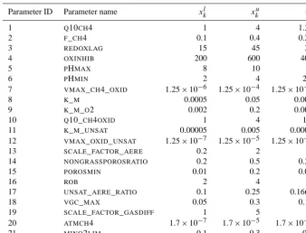
Table 1. CH4related parameters in CLM4.5bgc and their upper and lower boundsx_kuandxl_k, respectively, and the default parameter values

vk.

Parameter ID Parameter name x_kl xu_k vk

1 Q10CH4 1 4 1.33

2 F_CH4 0.1 0.4 0.26

3 REDOXLAG 15 45 30

4 OXINHIB 200 600 400

5 PHMAX 8 10 9

6 PHMIN 2 4 2.2

7 VMAX_CH4_OXID 1.25×10−6 1.25×10−4 1.25×10−5

8 K_M 0.0005 0.05 0.005

9 K_M_O2 0.002 0.2 0.002

10 Q10_CH4OXID 1 4 1.9

11 K_M_UNSAT 0.00005 0.005 0.0005

12 VMAX_OXID_UNSAT 1.25×10−7 1.25×10−5 1.25×10−6

13 SCALE_FACTOR_AERE 0.2 2 1

14 NONGRASSPOROSRATIO 0.2 0.5 0.33

15 POROSMIN 0.01 0.2 0.05

16 ROB 2 4 3

17 UNSAT_AERE_RATIO 0.1 0.25 0.1667

18 VGC_MAX 0.05 0.3 0.15

19 SCALE_FACTOR_GASDIFF 1 5 1

20 ATMCH4 1.7×10−7 1.7×10−5 1.7×10−6

21 MINO2LIM 0.1 0.3 0.2

emissions would dominate the sum (1a) because their RM-SEs would accordingly be larger. In that case the optimiza-tion would be driven by minimizing the RMSE of the site(s) with the largest emissions. There are also other methods of howwi could be determined. In the numerical experiments,

we will investigate also the possibilities of assigning equal weights to each observation site and assigning weights de-rived from grouping the observation sites into zones. Another possibility would be to apply clustering algorithms in order to determine groups of observation sites with similar char-acteristics. For this possibility, however, different clustering methods and different numbers of desired clusters will lead to different groups and different weight adjustments. Lastly, the problem could be formulated as multi-objective optimiza-tion problem, for example, with 16 objectives and the goal of minimizing each observation site’s RMSE individually, or as bi-objective optimization problem by minimizing the sum of the weighted RMSE values of northern and southern lo-cations at the same time. However, each objective function evaluation is very expensive, and thus the number of evalu-ations that can be done to obtain the Pareto front in a multi-objective setting is limited. Our focus is on demonstrating that single objective global optimization analysis is useful in identifying reasonable parameter values.

3 Methane-related parameters in CLM4.5bgc and sensitivity analysis

CLM4.5bgc has 21 parameters related to the methane emis-sion predictions. The parameter names, their upper and lower bounds, and default values are shown in Table 1. The upper and lower bounds have been derived based on reported val-ues in the literature (see Table C1 in Appendix C). How these parameters are used in the model is detailed in Riley et al. (2011) and Meng et al. (2012) and we repeat the important equations in Appendix A. The default parameter valuesvk

are available in the CLM4.5bgc (see Table 1).

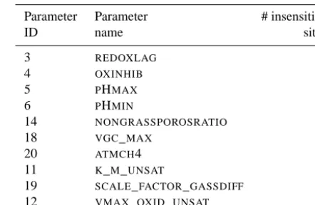
Optimization problems become increasingly more com-plex and difficult to solve as the number of parameters in-creases (curse of dimensionality). Thus, we determine first which of these 21 parameters are the most sensitive and thus the most important for the optimization. By sensitive we re-fer to parameters that when changed slightly lead to a signif-icant change in emission predictions. Insensitive parameters, on the other hand, can be changed and do not (or compara-tively only very mildly) change the emission predictions and can thus be excluded from the optimization, which decreases the problem dimension.

(6)

Table 2. Parameters that are sensitive for most observation sites (out

of 16).

Parameter Parameter # sensitive

ID name sites

1 Q10CH4 16

2 F_CH4 16

7 VMAX_CH4_OXID 16

13 SCALE_FACTOR_AERE 16

9 K_M_O2 15

15 POROSMIN 14

16 ROB 11

8 K_M 10

17 UNSAT_AERE_RATIO 10

10 Q10_CH4OXID 9

21 MINO2LIM 9

and we recorded the absolute change in emission predictions, i.e. we ran CLM4.5bgc with perturbed parameter values

(a) xk=min{vk+0.2(x_ku−x_kl), x_ku}, ∀k=1, . . ., dwhen

in-creasingvkfor 20 %, and

(b) xk=max{vk−0.2(x_ku−x_kl), xl_k}, ∀k=1, . . ., d when

decreasingvkfor 20 %

for each parameter separately.

There are several parameters that are relatively important to the sensitivity test for all 16 observation sites, but there are also parameters that are important for some locations and less important for others. Tables 2 and 3 show the sensitive and insensitive parameters together with the number of lo-cations (out of 16) for which these parameters are important and unimportant, respectively. Thus, in the optimization we consider only the parameters in Table 2 since these param-eters are the most important at most locations. Please note that, due to (nonlinear) relationships between the parame-ters, for many parameters the effects of individual param-eters will be opposite but act in a similar manner, indicat-ing that some parameters may be difficult to optimize for. In order to limit the number of parameters we consider, while allowing for the largest range in behavior, we combine in-formation from the sensitivity study with inin-formation about the methane flux equations themselves (described in more detail in Appendix A). The most important parameters from the sensitivity study come from the dominant three terms in the methane flux equation, which are production (parame-ters 1, 2, and 21), oxidation (parame(parame-ters 7, 8, 9, and 10), and aerenchyma transport (parameters 13, 15, 16, and 17). The first four parameters chosen are also the most important pa-rameters at all 16 sites (see Table 2). Because production is the most important term, there are two parameters from pro-duction that the sensitivity studies indicate are the most im-portant, namely one that controls globally the methane pro-duction flux (F_CH4, parameter 2), and one term that con-trols the temperature dependency of the methane production

Table 3. Parameters that are least sensitive for observation sites (out

of 16).

Parameter Parameter # insensitive

ID name sites

3 REDOXLAG 16

4 OXINHIB 16

5 PHMAX 16

6 PHMIN 16

14 NONGRASSPOROSRATIO 16

18 VGC_MAX 16

20 ATMCH4 15

11 K_M_UNSAT 13

19 SCALE_FACTOR_GASSDIFF 13

12 VMAX_OXID_UNSAT 10

(Q10CH4, parameter 1). Another parameter that influences methane at all the sites comes from the oxidation equation (VMAX_CH4_OXID, parameter 7), and the final parameter that is important at all 16 sites is the parameter controlling the aerenchyma transport (SCALE_FACTOR_AERE, param-eter 13). The above four paramparam-eters are the most sensitive parameters, and thus are easy to choose, as well as cover most of the important processes we want to investigate. For the last parameter, we include one parameter that controls how inundation affects methane production (MINO2LIM, pa-rameter 21). Inundation is an important process for control-ling methane flux, since there is an order of magnitude more methane coming from wet areas than dry, and thus having one parameter which changes the model’s sensitivity to in-undation is appropriate.

4 Surrogate models and surrogate model algorithms

4.1 Surrogate models

Surrogate models are used in optimization algorithms that aim to solve computationally expensive black-box problems. Surrogate models serve as computationally cheap approxi-mations of the expensive simulation model (Booker et al., 1999), i.e.,f (x)=s(x)+e(x), wheref (·)denotes the true expensive objective function,s(·)denotes the computation-ally inexpensive surrogate model, ande(·)denotes the dif-ference between both. Surrogate models are used throughout the optimization to guide the search for promising solutions. The computationally expensive objective function is evalu-ated only at few selected points, and thus it is possible to find near-optimal solutions with only very few expensive function evaluations.

(7)

Simp-son et al., 2001), polynomial regression models (Myers and Montgomery, 1995), and multivariate adaptive regression splines (Friedman, 1991). There are also mixture models (also known as ensemble models) that exploit information from several different surrogate model types (Goel et al., 2007; Müller and Piché, 2011; Müller and Shoemaker, 2014; Viana et al., 2009). In general any type of surrogate model may be used in a surrogate model optimization algorithm. In this study, we use RBFs because they have been shown to perform better in comparison to other surrogate model types (Müller and Shoemaker, 2014).

An RBF interpolant is defined as follows:

s(x)=

n

X

ι=1

λιφ (kx−xιk)+p(x), (6)

where φ (τ )=τ3 denotes the cubic radial basis function whose corresponding polynomial tail is linear (p(x)=b0+ bT_x_{), and}_x

ι, ι=1, . . ., n, denotes the points at which the

objective function has already been evaluated. The parame-tersλι∈R, ι=1, . . ., n, and the parametersb0∈Rand b=

[b1, . . ., bd] ∈Rd are determined by solving the following

linear system of equations:

8 P

PT 0

λ c = F 0 , (7)

where8ιν=φ (kxι−xνk),ι, ν=1, . . ., n, 0 is a matrix with

all entries 0 of appropriate dimension, and

P=      xT 1 1 xT 2 1 . . . . . . xT n 1      , λ=     λ1 λ2 . . . λn     c=       b1 b2 . . . bd b0      

, F=    

f (x1)

f (x2)

. . . f (xn)

   

. (8)

The matrix in Eq. (7) is invertible if and only if rank(P)=

d+1 (Powell, 1992).

4.2 Surrogate global optimization algorithm

Surrogate global optimization algorithms follow in general the steps shown in Algorithm 1.

We use the DYCORS algorithm by Regis and Shoemaker (2013) for the optimization of the methane-related param-eters of CLM4.5bgc. The reader is referred to this publi-cation for the details of the algorithm. Since the param-eters have significantly different ranges (see Table 1), we scale all parameters to the interval [0,1] when selecting new sample sites. When doing the computationally expen-sive CLM4.5bgc simulations, we scale the parameters back to their original ranges. Thus, the perturbation radius used in DYCORS is the same for each variable.

We create a symmetric Latin hypercube initial experimen-tal design with 2(d+1)points and run CLM4.5bgc at the selected parameter vectors in order to compute the objec-tive function values. We then fit the cubic RBF model to

Algorithm 1 General surrogate global optimization

algo-rithm

1: Select points from the variable domain to create an initial ex-perimental design.

2: Do the expensive objective function evaluations (here the CLM4.5bgc simulations) at the points selected in Step . 3: Fit the surrogate model (here the RBF model) to the data from

Steps and .

4: Use the information from the surrogate model to select the new evaluation pointxnew.

5: Do the expensive evaluation at xnew:fnew=f (xnew)(here, run CLM 4.5bgc for the parameter input vectorxnew). 6: if Stopping criterion is not met (the maximum number of

al-lowed function evaluations has not been reached) then 7: Update the surrogate model and go to Step . 8: else

9: Return the best solution found during the optimization. 10: end if

the data and generate two sets of candidate points for the next expensive function evaluation (the next CLM4.5bgc run at the 16 sites). The first set of candidate points is gener-ated as described by Regis and Shoemaker (2013) by ran-domly perturbing the best point found so far. The second set of candidate points is generated by uniformly selecting ran-dom points from the whole variable ran-domain. Thus, we create twice as many candidate points as DYCORS. The goal of us-ing uniformly random points from the whole variable domain is to obtain candidates that are far away from the best point found so far, and hence if selected as a new evaluation point, the search is more global (exploration by function evaluation at points that are far away from already sampled points).

We use the same criteria as in DYCORS for determining the best candidate point (using the RBF approximation to predict the objective function values at the candidate points, compute the distance of the candidate points to the set of already sampled points, and compute a weighted score of these two measures where the weights cycle through a pre-defined pattern). In order to guarantee that the matrix in Eq. (7) is well-conditioned, we ensure (as done in Regis and Shoemaker, 2013) that the sample points are sufficiently far away from previously evaluated points by discarding candi-date points that are closer than a given threshold distance to previously evaluated points. We run CLM4.5bgc at each of the 16 observation sites using the one newly selected sam-ple point as input parameter vector to obtain the correspond-ing objective function value. We update the RBF model with the new data and iterate until we have reached the maximum number of allowed function evaluations.

5 Numerical experiments

(8)

case), we generate synthetic (pseudo) data and treat it as if it were the real measurement data in order to assess how well our optimization approach performs. For these experiments we know the optimal solution. In the second set of experi-ments (real data case), we use the measured methane emis-sion data and apply the optimization algorithm. The goal in the second set of experiments is to find a parameter set that reduces the objective function value (the weighted RMSE in Eq. 1a) from its default value (the RMSE when using CLM4.5bgc’s default parameter settings, see also Table 1, column vk). Finally, we run CLM4.5bgc globally with the

best set of parameters found during the optimization of the real data case and investigate how much the default model predictions and the model predictions with the optimized pa-rameter values differ from each other.

We did experiments withd=5 andd=11 parameters re-spectively. For thed=5 experiments, we used parameters 1, 2, 7, 13, and 21 (Table 2). Thus, we have parameters related to three types of CH4 emission, namely oxidation

ter 7), aerenchyma (parameter 13), and production (parame-ters 1, 2, 21). For the 11-parameter optimization, we used all variables shown in Table 2.

For each set of experiments we ran the optimization algo-rithm three times in order to examine the influence of the ran-dom component in the algorithm (ranran-dom initial experimen-tal design and random generation of candidate points). We allowed 800 function evaluations for the five-dimensional problem and 1000 evaluations for the 11-dimensional prob-lem. The question of how many function evaluations need to be performed in order to obtain a fixed level of solution accuracy is problem dependent. For computationally expen-sive optimization problems, such as the problem we consider here, the time for evaluating the objective function and the totally available time for obtaining a solution usually defines how many evaluations can be done with any algorithm. Re-sults for many difficult computationally expensive optimiza-tion problems (for example, problems with multiple local minima) indicate that surrogate global optimization methods can usually obtain more accurate results compared to non-surrogate methods with the same limited number of evalua-tions (see, for example, Mugunthan et al., 2005). It is a very difficult problem to find the best values of the parameters for climate models, and the more evaluations one does, in gen-eral the better the answer.

The weightswi in Eq. (1a) were for the pseudo data case

computed based on the pseudo observations (see Sect. 5.1) at each of the 16 sites at the same dates for which we also have real measurements. For the real data case, the weights were computed based on the actual measurements. The weights are given in Table D1 in Appendix D.

Solving problem (1a) requires running CLM4.5bgc for each input vector x of parameter values and for each of the 16 observation sites. We run CLM4.5bgc on the Yellow-stone Supercomputing Facility (Computational and Informa-tion Systems Laboratory, 2012). Each simulaInforma-tion at a single

0 200 400 600 800

10−1

100

101

102

Number of function evaluations

Objective Function Value

T1 min RMSE: 0.28 T2 min RMSE: 0.46 T3 min RMSE: 0.40

Figure 1. Progress plot that shows the development of the best

ob-jective function value found vs. the number of function evaluations for the pseudo data case withd=5 parameters for optimization tri-als T1, T2, and T3. The legend shows the lowest RMSE value found in each trial.

location takes between 15 and 30 min. We do the simulations for the 16 sites in parallel in order to speed up the objective function evaluation time.

5.1 Pseudo data case

We assessed the performance of the optimization algorithm by investigating how well the algorithm could find the model parameters that were used for creating the pseudo data. For this purpose, we ran CLM4.5bgc with default parameter val-uesvk, k=1, . . ., d,at all 16 sites for the same time span for

which we also have observation data (see Tables B1 and B2 in Appendix B) and we record the model’s predictions for the same dates at which the methane emissions were measured. We use this as our pseudo observation data that we want to match in the optimization, i.e., the goal of the optimization is to start from a set of parameter vectors that is different from the default parameter values and to recover the default parameter values by optimization. For the default parameter values, the objective function value will be zero, which is the global minimum of the pseudo data case.

5.1.1 Results ford=5

(9)

Table 4. Default and optimized parameter values of optimization

trials T1, T2, and T3 for the five-dimensional pseudo data case. We report four decimal places because the model output is sensitive to very small changes for some variables. Note that we scaled the numbers to the interval [0,1].

Param. Default T1 T2 T3

1 0.1100 0.1088 0.1099 0.1091

2 0.5333 0.5366 0.5385 0.5458

7 0.0909 0.0912 0.0943 0.0967

13 0.4444 0.4461 0.4454 0.4443

21 0.5000 0.4936 0.4934 0.4856

RMSE 0 0.28 0.46 0.40

an approximation method), but the default parameter values are matched closely.

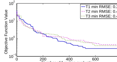
5.1.2 Results ford=11

Figure 2 shows the objective function value development as the number of function evaluations increases for the 11-dimensional case for the three trials T1, T2, and T3. The fig-ure shows a rapid decrease of the objective function value from over 50 to less than 10 within 100 evaluations, which shows that the surrogate model algorithm is very efficient at finding improved solutions. Although the objective function value improvement over the following function evaluations is lower, we can see that the algorithm still makes progress and if we allowed more than 1000 evaluations, the objective function value would be further improved (which also fol-lows from the global convergence property of the DYCORS algorithm).

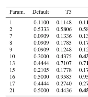
Table 5 shows the parameter values of the best of the three trials (T3) together with the default parameter values and the variable vector CP that was evaluated during the optimization and that has a worse objective function value than the best solution, but that is closer to the default parameter values. This point has the same parameter values as T3 for all but two parameters, namely, parameters 10 (Q10_CH4OXID) and 21 (MINO2LIM), which we indicate by bold numbers. For these two parameters, the point CP is closer to the global optimum, but it has a worse objective function value. This indicates a multimodality of the objective function (getting closer to the true global minimum requires an increase in the objective function value, i.e., the algorithm has to escape from a local basin of attraction). This multimodality makes the search for the global optimum significantly more difficult.

In order to examine the impact of the differences between default and optimized parameter values on the model predic-tion, we use the best parameter vector of each trial and plot the corresponding CH4emission predictions against the

pre-dictions when using the default parameter values in Figure 3. We can see that although we do not exactly match the default parameter values, the model’s predictions when using the

op-0 200 400 600 800 1000

100

101

102

ob-jective function value found vs. the number of function evaluations for the pseudo data case withd=11 parameters for optimization trials T1, T2, and T3. The legend shows the lowest RMSE value found in each trial.

Table 5. Default and optimized parameter values of optimization

trial T3 and parameter values for the point CP that was sampled during the same optimization trial and that is closer to the default point, but that has a worse objective function value (11-dimensional pseudo data case). Bold numbers indicate the parameters for which CP is closer to the default value than T3 (but CP has a worse objec-tive function value).

Param. Default T3 CP

1 0.1100 0.1148 0.1148

2 0.5333 0.5806 0.5806

7 0.0909 0.1336 0.1336

8 0.0909 0.1785 0.1785

9 0.0909 0.1248 0.1248

10 0.3000 0.4375 0.4302

13 0.4444 0.7107 0.7107

15 0.2105 0.1778 0.1778

16 0.5000 0.9583 0.9583

17 0.4444 0.2740 0.2740

21 0.5000 0.4436 0.4583

RMSE 0 2.28 2.35

timized parameters are very close to the predictions when us-ing the default parameter values (all points in the scatter plot lie close to or on the dashed line which represents agreement of default and optimized predictions). As also reflected in the best RMSE value reported in the legend, T3 matches the de-fault data best and T2 has the largest differences.

This result indicates that the calibration problem is not “identifiable” for all parameter sets, indicating that more than one parameter set can give a very similar result in terms of the objective function value. For example, for the model

y=α

βx+γ, there are many combinations of values forα

(10)

0 200 400 600 800 1000 1200 1400 0

200 400 600 800 1000 1200 1400

Prediction with default parameters

Prediction with optimized parameters

Figure 3. CLM4.5bgc CH4predictions when using the default

pa-rameter values vs. the predictions when using the best solution found in each of the three optimization trials T1, T2, and T3, re-spectively, for the pseudo data case withd=11 parameters. The legend shows the lowest RMSE value found in each trial.

some constantκ. With only five parameters as described in the previous section, the parameter values obtained from the optimization did match very closely with those of the default case used to create the pseudo data, and thus with this small set of parameters the problem was identifiable. However, for 11 parameters, we did encounter the identifiability problem. In some disciplines such parameters are called “hidden”. For example, estimatingα andγ in the previous example with

y=α

βx+γ whenβis given would be identifiable. However,

estimatingα,β, andγ is no longer identifiable.

It would be desirable to have an identifiable model, but the CLM (and probably other climate modules) have a number of interacting parameters and multiplicative nonlinearities, and thus there is no guarantee that all parameters are identifiable. This is reinforced by the data in Table 5, which indicates that the surface over which the optimization algorithm searches in the 11 parameter case is multi-modal, i.e., there are multiple local minima and it is possible for two (or more) parameter sets to yield the same objective function value (here RMSE). Hence the inability of the optimization to find the exact set of parameters that was used for generating the pseudo data is a problem caused by the complexity and multiplicative nonlinearities of the CLM model, not by the choice of the optimization method. However, the optimization analysis for both pseudo data cases (with 5 and 11 parameters, respec-tively) shows that the chosen optimization method is able to find a set of parameter values that has a low prediction error. The multi-modality in Table 5 does indicate the need for a global (not a local) optimization method.

5.2 Real data case

In the real data case, we use the actual methane emission measurements at each of the 16 observation sites for

com-0 50 100 150 200

110 115 120 125 130 135 140 145 150 155 160 165

ob-jective function value found vs. the number of function evaluations for the real data case withd=5 parameters for optimization tri-als T1, T2, and T3. The legend shows the lowest RMSE value found in each trial. The first function evaluation (left side of the graphs) corresponds to the RMSE when using the default parameters.

puting the objective function value. Since we only have very few observations for each site and no information about mea-surement errors, we did not exclude any of the meamea-surements from the optimization although there might be outliers. Also for the real data case we examine the case for d=5 and

d=11 variables.

5.2.1 Results ford=5

The progress of the development of the objective function value for the three trials T1, T2, and T3, respectively, is il-lustrated in Fig. 4 which also shows in the legend the lowest RMSE value found in each of the three trials. The RMSE was efficiently reduced from over 155 to below 115 within the first 150 function evaluations. Thereafter the objective func-tion value improvement was at a significantly lower rate. All three trials return a solution with approximately the same ob-jective function value.

The parameter values of the best solutions found in the three trials are shown in Table 6 where also the default pa-rameter values are given for comparison. We can see that the three optimized solutions are approximately the same and significantly different from the default case. We can also see that three of the five optimized parameter values are on or very close to the boundary of the variable domain (shown in bold), indicating that improvements of the objective func-tion value may be possible by increasing the parameter range. However, it is not possible due to physical constraints and at this point, we do not have information about possible wider parameter ranges than the ones we used in this study.

Figures 5 and 6 show the CH4 emission predictions of

(11)

wet-Table 6. Default and optimized parameter values of optimization

trials T1, T2, and T3 for the five-dimensional real data case. Bold indicates optimized parameters that are on (or close to) the variable boundary (all variables are scaled to [0,1]).

1 0.1100 0 0 0

2 0.5333 0.1705 0.1747 0.1699

7 0.0909 0.7878 0.7518 0.7865

13 0.4444 0 0 0.0267

21 0.5000 1 1 1

RMSE 156.40 114.24 114.11 114.24

19940 1994.5 1995 1995.5 1996 1996.5 1997

100 200 300 400 500 600

year

CH

4

Observations CLM default: 209.25 Optimized T1: 221.90 Optimized T2: 220.34 Optimized T3: 221.94

Figure 5. CH4emission observations and predictions when using

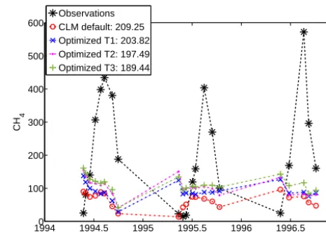
the optimized parameters of optimization trials T1, T2, and T3, re-spectively, and when using the default parameters for the wetland site Alberta, Canada, for the real data case withd=5 parameters. The legend shows the lowest RMSE value found in each trial.

land and one rice paddy site) together with the actual obser-vation data. The legends show the associated RMSE value before applying the weights for computing (Eq. 1a). We can see that the optimized solution actually worsens the predic-tions for Alberta (the RMSE value with default parameters is about 209 and with optimized parameters, the value is about 221, which is about 6 % worse). For Central Java, on the other hand, the RMSE values of the optimized solutions are significantly better than for the default values (the de-fault RMSE is about 221 and the optimized RMSE values are about 48, which is an improvement of over 350 %). In both figures we can also see that despite the large differences between optimized and default parameter values, the trend in the predictions of CLM4.5bgc is the same, i.e., when the predicted CH4emissions with default parameters increase so

do the predicted emissions when using the optimized param-eters and vice versa.

2001.80 2001.85 2001.9 2001.95 2002 2002.05 2002.1 2002.15 50

100 150 200 250 300 350 400

year

CH

4

Figure 6. CH₄emission observations and predictions when using

the optimized parameters of optimization trials T1, T2, and T3, re-spectively, and when using the default parameters for the rice paddy site Central Java, Indonesia, for the real data case withd=5 param-eters. The legend shows the lowest RMSE value found in each trial.

0 50 100 150 200 250 300 350 400

100 110 120 130 140 150 160 170

ob-jective function value found vs. the number of function evaluations for the real data case withd=11 parameters for optimization tri-als T1, T2, and T3. The legend shows the lowest RMSE value found in each trial. The first function evaluation (left side of the graphs) corresponds to the RMSE when using the default parameters.

5.2.2 Results ford=11

Figure 7 shows the progress plots for each of the three trials together with the best objective function values found (leg-end) for the 11-dimensional case. The best objective func-tion value found is about equal for each of the three trials. The figure shows that in each trial the algorithm is able to efficiently reduce the objective function value within the first 200 function evaluations. The improvement after 200 func-tion evaluafunc-tions is significantly slower.

(12)

exam-Table 7. Default and optimized parameter values of optimization

trials T1, T2, and T3 for the 11-dimensional real data case. Bold indicates optimized parameters that are on the variable bound (all variables are scaled to [0,1]).

1 0.1100 0 0 0

2 0.5 333 0.4220 0.3298 0.3813

7 0.0909 0.7093 0.6889 0.7260

8 0.0909 1 1 0.9754

9 0.0909 0 0.2335 0.6971

10 0.3000 0.7702 0.6195 0.6195

13 0.4444 1 1 0.8063

15 0.2105 0.6987 1 1

16 0.5000 0.0865 0.4274 0.2473

17 0.4444 0.8543 0.3113 0.5359

21 0.5000 0.5064 0.7449 0.5586

RMSE 164.46 107.24 107.58 107.41

ple, parameters 1, 7, and 8, all trials lead to approximately the same values (which are different from the default param-eter values). For the remaining paramparam-eters, the values cor-responding to the best solution found differ significantly for each trial and differ also from the default parameter values. Also for the 11-dimensional problem, some parameter values corresponding to the best solution found are on the upper or lower boundary of the parameter range (for example, param-eters 1, 8, 13, 15, indicated in bold).

Since all three solutions have approximately the same ob-jective function values, but the points differ greatly, it is an indicator that we either have a multi-modal surface in which some minima assume approximately the same objec-tive function values, or we have a very flat valley in which many points assume similar objective function values. Both possibilities make it very difficult for gradient-based opti-mization algorithms to find the global optimum. In the first case, the optimization algorithm will get trapped in a local optimum if it is not started close to the global minimum. In the second case, the gradient-based algorithm would require many function evaluations because many steps and gradient computations are necessary due to a very small step size. The surrogate optimization algorithm overcomes this problem.

Table 8 shows the unweighted RMSE values (before ap-plying the weights in Eq. (1a) for computing the objective function value) between observations and simulations using the default parameters (column 5), the best parameters of op-timization trial T1 of the 11-dimensional case (column 4), and the best parameters of trial T2 of the 5-dimensional case, respectively. The table shows that with our optimiza-tion we were able to decrease the default RMSE for four sites in the 5-dimensional case and for six sites in the 11-dimensional case. The RMSE is lower at seven sites for the 11-dimensional case than for the 5-dimensional case. Since we minimized a weighted sum of all RMSE values, it can

19940 1994.5 1995 1995.5 1996 1996.5 1997

100 200 300 400 500 600

year

CH

4

the optimized parameters of optimization trials T1, T2, and T3, re-spectively, and when using the default parameters for the wetland site Alberta, Canada, for the real data case withd=11 parameters. The legend shows the lowest RMSE value found in each trial.

2001.80 2001.85 2001.9 2001.95 2002 2002.05 2002.1 2002.15 50

100 150 200 250 300 350 400

year

CH

4

the optimized parameters of optimization trials T1, T2, and T3, re-spectively, and when using the default parameters for the rice paddy site Central Java, Indonesia, for the real data case withd=11 pa-rameters. The legend shows the lowest RMSE value found in each trial.

be expected that the RMSE at some locations may be worse for the optimized case than for the default case. We can see that for two of the improved sites (Java and Cuttack), the im-provement is very large, and thus the overall RMSE of the optimized solution is lower than for the default parameters.

Figures 8 and 9 show the observed CH4 emissions, the

(13)

opti-Table 8. Unweighted RMSE values for each site using the best parameters found during optimization trial T1 of thed=11 real data case and trial T2 of thed=5 real data case and with default parameter values.

Site Name Unweighted RMSE Unweighted RMSE Unweighted RMSE

d=5 d=11 default

1 Alberta 220.34 203.82 209.25

2 Florida 1247.70 1280.29 1180.99

3 Michigan 334.01 337.51 328.10

4 Minnesota 41.05 35.16 34.31

5 Nanjing 97.88 96.14 212.18

6 Vercelli 325.34 326.04 293.36

7 Texas 179.21 139.09 116.85

8 Japan 132.31 161.22 184.88

9 California 372.71 374.59 360.37

10 New Delhi 18.67 19.96 14.21

11 Beijing 66.79 60.89 56.99

12 Java 49.09 54.61 221.52

13 Chengdu 231.93 241.91 198.42

14 Cuttack 72.01 63.75 364.75

15 Panama 446.83 464.59 422.86

16 Salmisuo 156.79 132.16 146.52

Total RMSE 3792.66 3991.73 4345.56

1993.4 1993.5 1993.6 1993.7 1993.8 1993.9 1993.4 1993.5 1993.6 1993.70 50

100 150 200 250 300 350 400

year

CH

4

the optimized parameters of optimization trials T1, T2, and T3, re-spectively, and when using the default parameters for the wetland site Salmisuo, Finland, for the real data case withd=11 parame-ters. The legend shows the lowest RMSE value found in each trial.

mized parameters greatly improved the model’s predictions, but we can also see that the temporal variability in the pre-dictions stays the same although not as pronounced. We no-ticed this “temporal variability preserving” behavior for sev-eral sites such as Beijing, California, Cuttack, New Delhi, Florida, Japan, Michigan, Minnesota, Salmisuo, Texas, and Vercelli. Compared to the case where we optimized only five parameters, the solution for Alberta has improved and the RMSE values for all three trials are for thed=11 case better than the default RMSE value. On the other hand, the solution

100 101 102 103

100

101

102

103

Observation means

Simulated means

Default RMSE: 164.46 T1 min RMSE: 107.24 T2 min RMSE: 107.58 T3 min RMSE: 107.41

10

2

15 3

6

4 14

12 5 8

9 16

11

7 1

13

Figure 11. Scatterplot showing the mean values of the CH₄

predic-tions using the default and optimized parameter values of trials T1, T2, and T3, respectively, vs. the mean values of the observations. The numbers in the legend show the best RMSE value correspond-ing to each trial. The numbers above/below the boxes indicate the observation site ID (1: Alberta, 2: Florida, 3: Michigan, 4: Min-nesota, 5: Nanjing, 6: Vercelli, 7: Texas, 8: Japan, 9: California, 10: New Delhi, 11: Beijing, 12: Central Java, 13: Chengdu, 14: Cut-tack, 15: Panama, 16: Salmisuo).

for Central Java is worse for T1 in thed=11 case than in thed=5 case.

(14)

tri-Figure 12. Average methane emissions (mg CH4m−2d−1) simulated by CLM4.5bgc for (a) default parameters, (b) differences between de-fault parameters and 11-dimensional optimization trial T1, (c) differences between dede-fault parameters and optimization trial with unweighted sum of RMSE, and (d) differences between default parameters and optimization trial with zonally weighted sum of RMSE. Zonal means are shown on the right side of each spatial plot.

als although the best solutions found in the three trials were very different (see Table 7). Thus, it seems that the improve-ment of the model’s predictions is restricted by an underly-ing model component that enforces the temporal variability. This is likely to be associated with structural errors either in the methane or in the carbon model. Notice that the methane emission is dependent on the temporal variability predicted in the carbon and land model, especially on the heterotrophic respiration rate, which could have the wrong magnitude or temporal evolution.

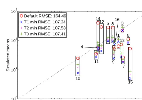
Figure 11 shows a scatter plot of the mean values of the CH4predictions using default and optimized parameter

val-ues vs. the mean valval-ues of the observed CH4emissions.

Ide-ally, if the simulated emissions agreed with the observations, all points would lie on the dashed line. Thus, the closer a point to the dashed line, the more simulation and observation are in agreement. The figure shows that with the optimized parameters, we obtain better or similar results for Beijing, Cuttack, Minnesota, Central Java, Nanjing, Japan, Salmisuo, Alberta, and Michigan. Although not all sites have been strictly improved by the optimization, the overall RMSE has been improved (indicated in the legend).

Figure 11 also shows that with default parameters, CLM4.5bgc predicts less CH4 emissions than observed for

both observation sites in the northern latitudes (Alberta, ID=1, and Salmisuo, ID=16), which is corrected by the optimization such that the mean emissions at these sites are closer to the dashed line. Thus, based on the observation data, CLM4.5bgc with default parameters does not predict enough emissions in the northern latitudes. On the other hand, CLM4.5bgc over-predicts the emissions for four

lo-cations, namely Cuttack (ID=14), Central Java (ID=12), Nanjing (ID=5), and Japan (ID=8), which are located in the tropical and/or subtropical zone. For those four locations, the predictions with the optimized parameters are closer in agreement with the observations. Hence, the observation data force the model predictions to increase in the northern lati-tudes and to decrease in the tropics. This can also be seen in Figs. 12 and 13 in the following section where we simu-lated the model globally and compared default and optimized model predictions for the individual zones (discussed below).

5.2.3 Gobal CH4emission simulations

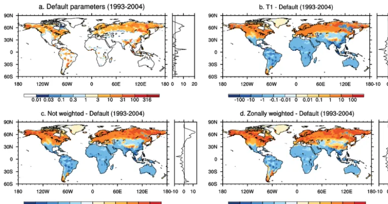
We simulated CLM4.5bgc to obtain predictions for the CH4 emissions on a global scale and compared the

predic-tions when using the default parameter values and the opti-mized parameter values from the 11-dimensional cases. Fig-ure 12 shows spatial plots of the average methane emissions (mg CH4m−2d−1) and the zonal means (right hand side of

the plots) when using the default parameters (panel a), and the difference between the predictions when using the default and the optimized parameters for trial T1 (panel b). The fig-ure shows that with the optimized parameters, the CH4

emis-sion predictions in the northern regions are larger than for the default parameters. For the tropics, the predictions with the optimized parameters are lower than when using the default values.

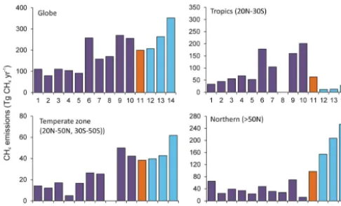
Figure 13 shows a comparison of the CH4emission

(15)

Figure 13. Comparison of total methane emissions (Tg CH4yr−1) between CLM4.5bgc and other models from natural wetlands. 1: Matthews and Fung (1987), 2: Aselmann and Crutzen (1989), 3: Bartlett et al. (1990), 4: Bartlett and Harriss (1993), 5: Cao et al. (1996), 6: Walter et al. (2001), 7: Bousquet et al. (2006), 8: Bloom et al. (2010), 9: CLM4Me, Riley et al. (2011), 10: CLM4Me’, Meng et al. (2012), 11: this study, CLM4.5bgc with default parameters, 12: this study, CLM4.5bgc withd=11 optimized parameters of T1, 13: this study, CLM4.5bgc withd=11 optimized parameters of unweighted sum of RMSE, and 14: this study, CLM4.5bgc with

d=11 optimized parameters of zonally weighted RMSE. Note that number 7 is a top-down approach and number 9 may include the rice paddy emissions. For number 8, no data were available for the tropics and the temperate zone.

default parameters (model 11). However, the predictions of CH4 emissions in the tropics are significantly lower than

for the default model and the predictions are also lower in comparison to all other models (1–10). On the other hand, for the northern latitudes, CLM4.5bgc with optimized pa-rameters predicts significantly more CH4emissions than the

default model and models 1–10 in the comparison. Hence, even though the global average of predicted emissions did not change much, the distribution of the predicted emissions between the tropical and the northern latitudes changed sig-nificantly.

As indicated in the previous section, the observation data drive the model to predict more CH4 emissions in

north-ern latitudes and fewer emissions in the tropics. We inves-tigated whether our weighting scheme in Eq. (1a) may give too much influence to individual observation sites or zones. Thus, we did an additional optimization trial of the parame-ters in Table 2 where we give each observation site the same weightwi=1,i=1, . . .,16 (“unweighted”). We also did a

second additional optimization trial of the parameters in Ta-ble 2 where we give each zone the same influence on the total RMSE in order to account for the location of the various ob-servation sites (“zonally weighted”). Thus, each location in the temperate zone (12 sites totally) haswi=1/36, and each

location in the northern (2 sites) and tropical (2 sites) zone, respectively, has the weightwi=1/6.

The spatial plots of the differences between the average methane emissions when using default and optimized pa-rameters for the unweighted trial are shown in panel c of Fig. 12, and the spatial plots of the differences when using the zonally weighted objective function is shown in panel d of Fig. 12. The figures show that for both additional trials, the CH4emissions in the northern latitudes are even further

increased. Moreover, the bars for models 13 and 14 in Fig. 13 show the total methane emissions of the unweighted and the zonally weighted trials, respectively. The zonally weighted trial increases the global emissions, which is caused by larger emission predictions in the temperate zone and the northern latitudes. In comparison to the default CLM4.5bgc predic-tions, the unweighted trial shows a decrease in the predicted emissions in the tropics and an increase in the predicted emis-sions in the northern latitudes. Thus, even though it is sug-gested that CLM4.5bgc with default parameter settings over-predicts the CH4emissions in high latitudes (Koven et al.,

2013), the observation data argue that the predictions should even be increased.

6 Conclusions

In this paper we used a surrogate optimization approach for calibrating the parameters of the methane module of the Community Land Model (CLM4.5bgc). Given only rel-atively few measurements at 16 observation sites (wetlands and rice paddies) our goal was to explore the use of a sur-rogate optimization method to improve the model prediction capability in a computationally efficient way by minimizing the root mean squared error between the measurements and the model’s predictions. We identified important methane-related parameters in CLM4.5bgc by doing a sensitivity anal-ysis and we were thus able to reduce the problem dimension from 21 to 11. We then used a surrogate optimization ap-proach for tuning the most important parameters in order to solve the problem. We investigated two cases, namely a prob-lem with five of the most important parameters and a probprob-lem with all 11 parameters, respectively.

(16)

optimization method because the objective function was ex-pensive to evaluate and has multiple local minima. The surro-gate has been shown to reduce the number of objective func-tion evaluafunc-tions (e.g. climate model simulafunc-tions) required to obtain accurate approximations of the global minimum and so it is designed for computationally expensive models like climate modules.

By conducting the simulations globally and comparing the average predicted emissions with default and optimized pa-rameters, we could show that the total global CH4emissions

did not change significantly.

However, the distribution of the predicted emissions be-tween latitudes changed significantly. The observation data force the optimized model’s CH4emission predictions in the

(17)

Appendix A: Model equations

The methane biogeochemical model used in this study is integrated in the Community Land Model version 4.5 (CLM4.5), which is the land component of the Community Earth System Model (CESM, Hurrell et al., 2013). As dis-cussed in more detail in Riley et al. (2011) and Meng et al. (2012), the model represents five primary processes relevant to methane emission predictions. These processes include methane production (P), oxidation (Roxic), ebullition (E),

transport through wetland plant aerenchyma (A), and diffu-sion through soil (F De) (described below). The methane gas

and aqueous phase concentrations (RC) in each soil layer of

each grid box is calculated at every time point using the fol-lowing equation:

∂RC

∂t =

∂F De

∂z +P−E+A−Roxic. (A1)

In the following sections we consider each of these terms in more detail.

A1 Methane production

Methane production (P) in the anaerobic portion of the soil column is related to the grid cell estimate of heterotrophic respiration from soil and litter corrected for various factors:

P =RH×F_CH4×Q10CH4×fpHfpES, (A2)

where RH is the heterotrophic respiration from soil and

litter (mol C m−2s−1), and F_CH4 is the baseline fraction of anaerobically mineralized C atoms becoming CH4 (i.e.,

CO2/CH4).RH is corrected for its soil temperature

depen-dence through a Q10 factor (Q10CH4), pH (fpH), redox

po-tential (fpE), and a factor accounting for the seasonal

inun-dation fraction (S).

We adjusted the fractional inundation in each grid cell to account for a changing redox potential.

fpE= filag(t )

fi(t )

, (A3)

where the redox potential factor fpE is computed based on

the fractional inundationfi(t )and the adjusted fractional

in-undationfilag(t )that is producing methane.

The adjusted fractional inundationfilag(t )is computed as

filag(t )=fi(t )−fredox(t ), (A4)

where

fredox(t )=fi(t )−fi(t−1)

+fredox(t−1)

1− 1t

REDOXLAG

(A5) is the fraction of the grid cell where alternative electron ac-ceptors (such as O2, NO−3, Fe

+3_{, SO}2−

4 etc.) are consumed

(methane production is completely inhibited),1t is the time step, andREDOXLAGis the time constant parameter.

In the non-inundated fraction of a grid cell, we estimated the delay in methane production as the water table depth in-creases by estimating an effective depth below which CH4

production can occur (Zilag):

Zilag(t )=Zi(t )−Zredox(t ), (A6)

where

Zredox(t )=Zi(t )−Zi(t−1)

+Zredox(t−1)

1− 1t

REDOXLAG

(A7)

is the depth of the saturated water layer where alternative electron acceptors are consumed at timet andZi(t )is the

actual water depth at timet.

Additionally, we constrained the methane production us-ing the soil pH functionfpHwhich is represented as

fpH=10−0.2335pH

2₊_2.7727pH₋_8.6

, (A8)

where pH represents the soil pH. fpH is bounded by

two parameters, namely PHMIN and PHMAX (i.e., P

H-MIN< pH<PHMAX). The maximum methane production oc-curs at pH≈6.2.

We used a scaling factor (S) to mimic the impacts of sea-sonal inundation on methane production which is represented as

S=MINO2LIM(f−f )+f

f , S≤1, (A9)

where f and f are the instantaneous inundation fraction and annual average inundation fraction weighted by het-erotrophic respiration,MINO2LIMis the anoxia factor that re-lates the fully anoxic decomposition rate to the fully oxygen-unlimited decomposition rate.

A2 Methane oxidation

Methane oxidation (Roxic) is represented with double

Michaelis-Menten kinetics:

Roxic=VMAX_CH4_OXID

_C

CH4

K_M+CCH4

_C

O2

K_M_O2+CO2

Q10_CH4OXID×Fϑ, (A10)

where VMAX_CH4_OXID is the maximum oxidation rate (mol m−3s−1), Q10_CH4OXID is the temperature depen-dence of the reaction,K_MandK_M_O2 are the half satura-tion coefficients with respect to CH4and O2concentrations

(mol m−3),CCH4 andCO2 are the methane and oxygen

(18)

limitation factor for oxidation applied above the water table to represent water stress for methanotrophs.

Fϑis represented as: Fϑ=exp

₋_P

PC

, (A11)

where P andPC are the soil moisture potential and

opti-mum water potential (−2.4×105mm). If the soil layer is above the water table, the soil moisture limitation factorFϑ

is applied. To account for high-CH4-affinity methanotrophs

in upland soils, we used a lower oxidation rate constant

(VMAX_OXID_UNSAT) and half saturation coefficient with

respect to CH4concentrations (K_M_UNSAT).

A3 Methane transport through plant aerenchyma

The diffusive transport through aerenchymaA(mol m−2s−1) from each soil layer is represented in the model as:

A= C(z)−Ca

ra+ROB_{DpT ρ}×z

f

, (A12)

where D is the free-air gas diffusion coefficient (m2s−1),

C(z)andCaare the gaseous concentrations at depthzand at

the atmosphere (mol m−3_),_r

ais the aerodynamic resistance

between the surface and the atmospheric reference height (s m−1_), _ROB _{is the ratio of root length to vertical depth}

(obliquity),p is the porosity, T is the specific aerenchyma area (m2m−2), and ρf is the root density as a function of

depth. Oxygen concentrations can also diffuse into the soil layer from the atmosphere via the reverse of the CH4

path-way.

Here, aerenchyma porosity is parameterized based on the plant functional types (PFTs). A ratio is used to multiply up-land vegetation aerenchyma porosity by comparing to inun-dated systems:

p=p×UNSAT_AERE_RATIO (A13)

If the PFT is c3_arctic_grass, c3_nonarctic_grass, or c4_grass, then p=0.3. For the remaining PFTs, the poros-ity is multiplied by NONGRASSPOROSRATIO (ratio of root porosity in non-grass to grass):

p=p×NONGRASSPOROSRATIO. (A14)

A minimum aerenchyma porosity is set to 0.05. Therefore,

pis modified as:

p=max{p,POROSMIN}. (A15)

The aerenchyma area varies over the course of the grow-ing season. Therefore, it is parameterized usgrow-ing the simulated leaf area index as

T =fNNaL 0.22 π R

2_, _(A16)

whereLis the leaf area index (m2m−2) (used from CLM4.5 model simulation),Na is the maximum annual net primary

production (NPP, mol m−2s−1),R is the aerenchyma radius (2.9×10−3m), andfN is the below-ground fraction of the

current NPP.

The aerenchyma areaT is multiplied by a scale factor to adjust it:

T =T×SCALE_FACTOR_AERE. (A17)

The default value is 1.

A4 Methane ebullition

The representation of the ebullition fluxes in the methane model is based on Wania et al. (2010). The simulated aque-ous CH4concentration in each soil level is used to estimate

the expected equilibrium gaseous partial pressure as a func-tion of temperature and pressure. When this partial pressure exceedsVGC_MAX, bubbling occurs to remove CH4to

be-low this value, modified by the fraction of CH4 in the

bub-bles (taken as 57 %). TheVGC_MAXparameter is the ratio of saturation pressure triggering ebullition.

A5 Aqueous and gaseous diffusion

Gaseous diffusivity in the soil depends on several factors such as molecular diffusivity, soil structure, porosity, and or-ganic matter content. The relationship between effective dif-fusivity (De, m2s−1) and soil properties is represented as

De=D0θa2

_θ

a θs

3_b

×SCALE_FACTOR_GASSDIFF, (A18)

whereθa andθs are the air-filled and saturated water-filled

porosity, b is the slope of the water retention curve, and

SCALE_FACTOR_GASSDIFF is the scale factor for the gas

(19)

Appendix B: Observation sites

Tables B1 and B2 show the information about the wet-land and rice paddy observation sites, respectively, where methane emissions have been measured.

T able B1. W etland site data. P = precipitation, T = temperature. Site Name Location T ime W etland type Dominant v egetation Mean P & T Soil and climate characteristics Meas. techniques F orcing data sets ∗ References Michig an, USA 42.45 ◦N, 84.00 ◦W 1991–1993 Ombrotrophic peatland Sphagnum, Scheuchzeria palustris, V accinium oxycoccos P : 761 mm (1948–1980) Soil pH: 4.2 Static chamber Measured WT positions Shannon and White (1994 ) Minnesota, USA 47.53 ◦N, 266.33 ◦E 1991–1992

Poorly minerotrophic to

ombrotrophic

peatland

Sphagnum, Chamaedaphne calyculata,