Integration of prognostic aerosol–cloud interactions in a chemistry
transport model coupled offline to a regional climate model
M. A. Thomas1, M. Kahnert1,2, C. Andersson1, H. Kokkola3, U. Hansson1, C. Jones1,4, J. Langner1, and A. Devasthale1
1Research Department, Swedish Meteorological and Hydrological Institute, Folkborgsvägen 17, 60176 Norrköping, Sweden 2Department of Earth and Space Sciences, Chalmers University of Technology, 41296 Gothenburg, Sweden
3Finnish Meteorological Institute, Kuopio, Finland
4National Centre for Atmospheric Science, School of Earth and Environment, University of Leeds, LS2 9JT Leeds, UK
Correspondence to: M. A. Thomas (manu.thomas@smhi.se)
Received: 25 November 2014 – Published in Geosci. Model Dev. Discuss.: 03 February 2015 Revised: 08 June 2015 – Accepted: 12 June 2015 – Published: 30 June 2015
Abstract. To reduce uncertainties and hence to obtain a bet-ter estimate of aerosol (direct and indirect) radiative forc-ing, next generation climate models aim for a tighter cou-pling between chemistry transport models and regional cli-mate models and a better representation of aerosol–cloud in-teractions. In this study, this coupling is done by first forc-ing the Rossby Center regional climate model (RCA4) with ERA-Interim lateral boundaries and sea surface temperature (SST) using the standard cloud droplet number concentration (CDNC) formulation (hereafter, referred to as the “alone RCA4 version” or “CTRL” simulation). In the stand-alone RCA4 version, CDNCs are constants distinguishing only between land and ocean surface. The meteorology from this simulation is then used to drive the chemistry transport model, Multiple-scale Atmospheric Transport and Chemistry (MATCH), which is coupled online with the aerosol dynam-ics model, Sectional Aerosol module for Large Scale Ap-plications (SALSA). CDNC fields obtained from MATCH– SALSA are then fed back into a new RCA4 simulation. In this new simulation (referred to as “MOD” simulation), all parameters remain the same as in the first run except for the CDNCs provided by MATCH–SALSA. Simulations are car-ried out with this model setup for the period 2005–2012 over Europe, and the differences in cloud microphysical proper-ties and radiative fluxes as a result of local CDNC changes and possible model responses are analysed.
Our study shows substantial improvements in cloud micro-physical properties with the input of the MATCH–SALSA derived 3-D CDNCs compared to the stand-alone RCA4
1 Introduction
The scientific understanding of the climate effects of the dif-ferent aerosol species as well as their representation in mod-els and their physical and chemical transformation under dif-ferent meteorological conditions is still low (Boucher et al., 2013). Aerosols have a direct radiative effect by scattering and absorbing shortwave and long-wave radiation, thereby changing the reflectivity, transmissivity and absorptivity of the atmosphere. They can further act as cloud condensation nuclei (CCN), thereby influencing the microphysical proper-ties of clouds. This, in turn, can impact the optical properproper-ties and lifetimes of clouds, thus indirectly affecting the radia-tive properties of the atmosphere (Penner et al., 2004). Apart from ambient conditions, the ability of the aerosols to act as CCN depends on the size distribution (Dusek et al., 2006) and, for particles in the size range between 40 and 200 nm, on the chemical composition and mixing state (McFiggans et al., 2006).
The direct effect of aerosols and, even more so, their in-direct impact on radiative forcing have been identified as the largest sources of uncertainty in quantifying the radia-tive energy budget and its impact on climate system (Forster et al., 2007). An accurate estimate of these effects requires the coupling of atmospheric chemistry/aerosols to global cir-culation models (GCMs); however, due to their coarse res-olution, their accuracy reduces when one starts to zoom into regional scales. Hence, the recent generation of mod-els uses the regional climate modmod-els at a higher horizontal and vertical resolution instead of GCMs, for example, WRF-Chem (Grell et al., 2005), ENVIRO-HIRLAM (Baklanov et al., 2008), RegCM3-CAMx (Huszar et al., 2012; Qian and Giorgi, 1999; Qian et al., 2001). Recently, Baklanov et al. (2014) summarized the status of the online/offline European coupled meteorology and chemistry transport models with varying degrees of complexity in the representation of dy-namical and physical processes, aerosol–cloud–climate in-teractions, radiation schemes, etc. The main conclusion was that an online integrated modelling approach is the future and can be adapted to several modelling communities such as climate modelling and air-quality-related studies depend-ing on the objective of the study (Baklanov et al., 2014, and the references therein). The study also showed that for cli-mate modelling, the inclusion of feedback processes is the most important and significant improvements were notice-able in climate–chemistry/aerosols interactions. Whether the coupling need to be online or offline depends on the spe-cific study. For example, Folberth et al. (2011) showed that in long-lived greenhouse gas forcing experiments, the online approach did not give significant improvements, whereas for short-lived climate forcers, aerosols in particular, the online approach is very beneficial. The aerosol–cloud interactions, in particular, are either implicity or explicitly included in all online models. Schemes (e.g. Abdul-Razzak and Ghan, 2002) that explicitly resolve the activation of CCN to cloud
droplets are currently included only in a handful of online coupled models (ENVIRO-HIRLAM, WRF-Chem, etc). In-stead, the droplet number concentrations are derived empiri-cally and are used in the parameterization of droplet radii and autoconversion processes.
Here, we attempt a similar approach by adapting the Rossby Center regional climate model (RCA4) for the offline ingestion of cloud droplet number concentrations (CDNCs) from the cloud activation module embedded in the chemistry transport model, Multiple-scale Atmospheric Transport and Chemistry (MATCH), that is coupled online to the aerosol dynamics model, Sectional Aerosol module for Large Scale Applications (SALSA). Such a setup is useful in many ways: 1. A more detailed description of the emissions, transport, particle growth, deposition and aerosol processes can be included so as to obtain an accurate evaluation of aerosol radiative effects on a higher spatial resolution compared to global models (Colarco et al., 2010). 2. It is possible to assess the level of detail that is required
to describe the effects on a regional scale.
3. It can be used to assess the effects of future climate change on air quality.
In this paper, we present the results from a full fledged work-ing version of the couplwork-ing between a chemistry transport model (CTM) with a detailed aerosol dynamics model and a regional climate model. The coupling between these two model systems is offline and is done through CDNCs cal-culated by the CTM. The drawback of offline coupling is that there is no feedback on the simulation of chemistry and aerosols from changes in meteorology due to altered CDNC/radiation and no coupling to sea surface temperature (SST). In the following subsections, we introduce the models used in this study, their coupling and the improvements made in the cloud microphysical properties and radiative forcing.
2 Description of the models and experimental setups 2.1 Description of the models
Figure 1. Schematic showing the different model components and their couplings.
A sectional representation of the aerosol size distribution is considered and has three main size regimes (a: 3–50 nm, b: 50–700 nm and c:>700 nm) and each regime is again subdi-vided into smaller bins and into soluble and insoluble bins adding up to a total of 20 bins. A schematic of the sec-tional size distribution and the aerosol species considered in each bin is shown in Fig. 2. Anthropogenic emissions such as primary particulate matter (PM), NOx, NMVOC (Non-methane volatile organic compounds), SOx, NH3and carbon monoxide, volcanic and DMS (Dimethyl sulfide) emissions are taken from the EMEP expert emissions inventory for the year 2003. The aerosol and gaseous concentrations at the lat-eral and top model boundaries are set as described in An-dersson et al. (2007). The boundary concentrations are based on both observations at background locations and large-scale model calculations and are prescribed as monthly or season-ally varying fields. However, the boundary concentrations of organic matter (OM) are set to the seasonally varying mass size distributions and totals of marine OM as described in O’Dowd et al. (2004). The aerosol number concentrations are also introduced at the southern, western and northern lat-eral boundaries. These values are prescribed at the first model level and interpolated linearly to the top and eastern bound-aries where the concentrations are set to zero. Primary PM is divided into EC (elemental carbon), OC (organic carbon) and other emissions. This division of the primary PM is based on the TNO-MACC (TNO-Monitoring Atmospheric Composi-tion and Climate) emissions of EC and OC (Kuenen et al., 2011; Pouliot et al., 2012; see also the MACC project web page http://www.gmes-atmosphere.eu/). The emissions were given as annual totals. Seasonal, weekday and diurnal varia-tions of the emissions are sector specific and based on results from the GENEMIS (Generation and Evaluation of Emission Data) project (http://genemis.ier.uni-stuttgart.de/; Friedrich and Reis, 2004). The vertical distribution is also sector spe-cific and based on the vertical distribution used by the EMEP
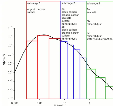
Figure 2. Schematic of sectional distribution of aerosol size bins and the chemical components in the bins (taken from Kokkola et al., 2008).
model. The particle emissions of EC and OC are distributed over different particle sizes according to sector resolved mass size distributions described by Visschedijk et al. (2009); see Andersson et al. (2015) for more details on how the emis-sions are distributed. Particulate nitrogen is described out-side SALSA, i.e. ammonium salts are not taken into account in the modelling of the aerosol microphysical processes. The lack of ammonium nitrate condensation in the aerosol mi-crophysics could cause underestimation of CDNC. Currently there are no parameterizations available that take into ac-count co-condensation of ammonia and nitric acid. Isoprene emissions are modelled online depending on the meteorology based on the methodology by Simpson et al. (1995). The ter-pene emissions (α-pinene) are taken from the modelled fields by the EMEP model. Sea salt is parameterized following the scheme of Foltescu et al. (2005) but modified for varying par-ticle sizes. This means that Mårtensson et al. (2003) is used if the particle diameter is≤1 µm otherwise Monahan et al. (1986) is used.
veloc-ity and turbulent kinetic energy (TKE) for stratiform clouds (Lohmann et al., 1999) derived from the RCA4 simulation. These CDNCs are then offline coupled to a regional climate model, RCA4 (Samuelsson et al., 2011), that provides us in-formation on cloud microphysical properties such as cloud droplet radii, cloud liquid-water path as well as radiative fluxes. In the stand-alone version of RCA4, the total number of cloud particles were set to constant values over the whole domain based on whether the surface is oceanic (150 cm−3) or land (400 cm−3) and scaled vertically. These constant val-ues were further used in calculation of effective radius of cloud droplets and in the autoconversion process (conver-sion of cloud droplet to rain). In this work, the 3-D CDNC fields obtained from the cloud activation model in MATCH– SALSA are now used in the RCA4 simulation.
2.2 Experimental setup – 1
For the simulations, RCA4 is run with 6-hourly ERA-Interim meteorology on lateral boundaries and sea surface tempera-ture and the 3-hourly RCA4 meteorological fields along with fields necessary to compute the updraft velocity are used to drive the MATCH–SALSA-cloud activation model. The aerosol properties are used in the cloud activation model to derive the 6-hourly CDNCs which are then employed to re-run RCA4 with dynamic rather than prescribed CDNCs to obtain cloud microphysical properties and radiative effects. The CDNC data are interpolated at every time step in the RCA4 model. Simulations were carried out with this model setup at 44 km×44 km spatial resolution for the European domain and 24 levels in the vertical (up to 200 hPa) for an 8-year period (2005–2012). Here, we look into the im-provements in the cloud microphysical properties and radia-tive fluxes with the incorporation of dynamic CDNCs where only local land surface fluxes can respond to these changes, hereby referred to as the MOD simulation. These results are compared with the control simulation, hereby referred to as the CTRL simulation in which the stand-alone version of RCA4 is used.
2.3 Experimental setup – 2
To evaluate the indirect aerosol effects due to the present-day (PD) anthropogenic aerosols, the pre-industrial (PI) emis-sions required for this simulation were taken from those de-veloped for the ECLAIRE project (effects of climate change on air pollution impacts and response strategies) for the year 1900 (http://www.eclaire-fp7.eu). The PI anthropogenic pre-cursor emissions were provided for CO, NH3, NOx, SOxand volatile organic compound (VOC). Other emissions such as biogenic emissions, DMS and volcanic are kept the same as in the original model setup. The particulate organic matter emissions are reduced to 14 % of the current emission lev-els in the pre-industrial setup based on the study by Carslaw et al. (2013). Simulations were carried out at the same spatial
resolution as in the previous setup and for the same European domain and for the same meteorology from 2005 to 2012. Here, we address the changes in cloud properties with respect to the emissions from the PI period without the climate feed-backs and we analyse the total radiative forcing. To evaluate the individual contribution from the first and second indirect aerosol effects to the total radiative forcings, two additional simulations each (for PI and PD climate) were carried out. We turn off the individual indirect aerosol effects (IAEs) by prescribing the constant CDNC values for the calculation of one IAE at a time; for example, to evaluate the sole contribu-tion from the first IAE, 3-D CDNC fields are used in the com-putation of cloud droplet (CD) radius to assess the changes in cloud albedo (first IAE) and constant CDNC values are used in the scheme for the autoconversion process (second IAEs) and vice versa.
3 Model evaluation and results 3.1 Aerosol number concentrations
Figure 3 shows the spatial distribution of the seasonal mean accumulation mode aerosol number concentrations from MATCH–SALSA model simulations driven by RCA4 mete-orology. The main contribution to accumulation mode par-ticles are from SO2−4 , EC, OC, sea salt and mineral dust. In the figure, emphasis is given to accumulation mode par-ticles as they can act as CCN and, depending on the wa-ter availability and updraft velocity, be efficiently converted into cloud droplets. A clear seasonality is noticeable with the highest concentrations during the summer months and low-est during the winter months. Concentrations reach as high as 600 cm−3over the southern European subcontinent during summer. This may be partly due to relatively large emissions of primary fine particles and gaseous SOx(Spracklen et al., 2010; Yu and Luo, 2009), and partly due to less precipitation in southern Europe compared to the rest of Europe resulting in longer residence times of these particles in the atmosphere (Andersson et al., 2013, 2015).
3.2 Cloud droplet number concentrations
Figure 3. Averaged aerosol number concentrations in the accumu-lation mode (cm−3).
in these regions. Residential biomass burning is more promi-nent in late autumn–winter–early spring months over east-ern Europe and Russia. Whereas, biogenic VOC emissions are higher in these regions during the summer season (Yt-tri et al., 2009, 2014). This is reflected in the higher CDNCs over these regions during these seasons.
Storelvmo et al. (2009) showed that differences in the cloud droplet activation would account for about 65 % of the total spread in shortwave forcing. So, it is important to see if this model setup reproduces the spatial distribution of CD-NCs realistically. The high droplet concentrations simulated over land compared to oceans agrees well with the previous studies of Barahona et al. (2011) and Moore et al. (2013). Zeng et al. (2014) analysed the CDNCs from the Moderate Resolution Imaging Spectroradiometer (MODIS) and Cloud-Aerosol Lidar with Orthogonal Polarization (CALIOP) sen-sors and it is evident that the droplet concentrations over the European subcontinent would be on an average between 150 and 200 cm−3, and over oceans the concentrations are as low as 100 cm−3. This agrees well with our simulations.
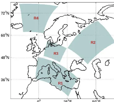
To understand the vertical distribution of CDNCs, we se-lect the following four regions as in Fig. 5 – R1: Mediter-ranean R2: eastern Europe R3: central Europe and R4: north-ern Atlantic. Figure 6 shows the joint histograms of CDNC and height (in km) over the four selected regions for win-ter (DJF) and summer (JJA) months. The colour scale shows the normalized frequency and the deeper shade means there is a high probability for the occurrence of those values. It can be seen that the majority of the CDNC values are less than 500 cm−3, but occasionally values also reach as high as 800 cm−3 irrespective of season and region. The figures also show an interesting seasonality of the PDFs (probabil-ity distribution functions) of CDNC. For example over the Mediterranean (R1) two peaks can be observed in summer, one around 3 km and another in the boundary layer;
how-Figure 4. Seasonal mean in-cloud averaged cloud droplet number concentrations (cm−3).
ever, in winter, only one peak is present and is located below 2 km. This is mainly due to the stronger vertical mixing of aerosols together with increased buoyancy and convection in summer. It is well known that the frequency of occurrence of very low level water clouds is high over this region during summer, while, in winter, the baroclinic disturbances lead to northward transport of winter storms over this region. Over eastern Europe (R2) and central Europe (R3), the height at which maxima of CDNCs occur is around 1.5 km in sum-mer, whereas during winter, the maxima is in the boundary layer. The droplet concentrations can vary widely over east-ern Europe compared to over central Europe where the con-centrations are mostly towards the higher side irrespective of the seasons. The opposite is observed over the northern At-lantic (R4) with a maxima of CDNCs simulated at around 1.5 km in winter and in the boundary layer in summer. This can be attributed to the long-range transport of pollutants from across the Atlantic observed during the winter months (HTAP, 2010).
3.3 Cloud droplet radii
As mentioned in Sect. 2, both the CTRL and MOD simu-lations follow the same parameterization scheme of Wyser et al. (1999) in the radiation and are formulated in Eq. (1). The effective radius for spherical droplets is estimated as
re,water= 3CC 4π ρlkN
, (1)
sur-Figure 5. Schematic of the four regions selected for this study. R1 – Mediterranean; R2 – eastern Europe; R3 – central Europe; R4 – northern Atlantic.
Figure 6. Seasonality in the vertical distributions of CDNC (cm−3) shown as joint histograms averaged over winter averaged (DJF) months (first column) and summer averaged (JJA) months (second column) for the selected four regions. The colour scale indicates the normalized frequency.
face; however, in the MOD simulation dynamic CDNCs are used.
The winter and summer mean cloud droplet radii in liq-uid water clouds for the MOD simulation (top row) and the CTRL simulation (second row) is discussed in Fig. 7. At first glance, apart from the spatial differences, one notices the strong disparity in the range of the radii values. In the MOD
Figure 7. Seasonal mean CD radii (µm) averaged over the entire water cloud for DJF mean and JJA mean in the MOD simulations (top row) and CTRL simulation (second row). Note the difference in scale.
simulation, CD radii reach as high as 13 µm, whereas in the CTRL simulation, the maxima observed is 5 µm. It can be seen that the radii of the droplets are much lower in the sum-mer months compared to the winter months basically due to the increased pollution during summer resulting in smaller droplets.
In Fig. 8, the joint histograms of CD radii and height dur-ing the summer over the Mediterranean and eastern Europe in MOD simulation are shown. The corresponding pattern in the CTRL simulation is shown as the solid line. It can be seen that the CTRL simulation does not exhibit any variability. However, the MOD simulation shows a distinct variability in height and range. It can be seen that over the Mediterranean and over Eastern Europe, a wide range of droplet radii can be observed from as low as 5 up to 16 µm and the larger droplets are present at around 2.0–4.0 km. However, there is a higher probability of observing larger droplets over eastern Europe compared to the Mediterranean.
The critical droplet radius at which large-scale precipita-tion occurs is set to 10 µm in the microphysics scheme. This would mean that with these low CD radii values obtained in the stand-alone RCA4 model, precipitation would be absent. It is important to note that the plotted CD radii values are de-rived from the model radiation scheme (i.e. this is the radia-tively active CD radii). For more details, refer Appendix A. 3.4 Cloud liquid-water path
com-Figure 8. Joint histograms of CD radii (µm) vs height averaged over JJA months in MOD simulation and the solid line shows the same in CTRL simulation. The colour scale shows the normalized fre-quency.
Figure 9. The difference in the vertically integrated cloud water in the MOD simulation compared to the CTRL simulation expressed as a percentage over the winter (DJF) and summer (JJA) months.
pared to the CTRL and vice versa. It can be seen that during the winter months, there is a significant decrease (up to 25 %) in the vertically integrated cloud liquid water over land and a slight increase over the water bodies when the 3-D CDNCs are used. However, during the summer months, the pattern is reversed with a noticeable increase in the CLWP over most of the European subcontinent. The decrease in the CLWP with increase in CD radii is consistent and may be partly at-tributed to precipitation removal. In the model, the critical droplet radius at which autoconversion becomes efficient is set to 10 µm. When the CD effective radius exceeds this crit-ical droplet radius, precipitation occurs. However, over land during summer, an increase in the CLWP is observed and can be partly due to the fact that the increase in CD radius is not sufficient to trigger precipitation.
We evaluated model simulated cloud liquid-water path es-timates using satellite sensor retrievals. We selected the liq-uid water path (LWP) for evaluation as it is tightly con-nected not only to other microphysical properties of clouds but also to the first and second indirect aerosol effects, which are the main application focus of the coupling attempted here. We used a decade-long data record (2003–2012) from the MODIS sensor flying onboard NASA’s Aqua satellite since 2002 (Platnick et al., 2003; Hubanks et al., 2008). The monthly level 3 data from the collection 5 are analysed over the study area for the boreal summer months of JJA (June, July and August), when liquid clouds are most prevalent and the quality of satellite retrievals is also best. The comparison
Figure 10. Spatial comparison of the simulated cloud liquid-water path (g m−2) (CTRL and MOD) with observations from the MODIS sensor onboard the Aqua satellite for the JJA months.
is shown as spatial distributions in Fig. 10 and as probabil-ity densprobabil-ity functions of the LWP in Fig. 11 as they cover the whole range of LWP values. We observe substantial im-provement in the distribution of LWPs in the MOD simula-tion compared to the CTRL-simulasimula-tion. The inclusion of the chemistry–aerosol–cloud microphysical link leads to a more realistic distribution of LWPs that is closer to the observa-tions. At the lower end of the distribution, the model simu-lates more optically thin liquid water clouds compared to the observations, more predominantly over southern Europe as can be seen in Fig. 10. But the LWP of optically thick clouds, which are most abundant and play a key role in the radiation budget over the study area, shows substantial improvements in the MOD simulation.
3.5 Total radiative fluxes at the top of the atmosphere The difference in the annual mean total net fluxes at the top of the atmosphere (TOA) due to these changes in the cloud microphysical properties is shown in Fig. 12. A significant change is seen over most of the domain with decreases up to
−5 W m−2when the CDNC values are assigned fixed num-bers depending on the underlying surface.
To evaluate the TOA radiative fluxes, we used a decade-long data for comparison from the Clouds and the Earth’s Ra-diant Energy System (CERES) sensor that is flying onboard Aqua satellite as well (Wielicki et al., 1996) (More informa-tion is available at http://ceres.larc.nasa.gov/documents/DQ_ summaries/CERES_EBAF_Ed2.8_DQS.pdf). The level 3 Energy Balanced and Filled estimates of all-sky net top of the atmosphere (EBAF-TOA, Edition 2.8) fluxes are analysed for comparison with MOD and CTRL simulations and shown in Fig. 13. The distribution of fluxes in the MOD simulation is closer to the CERES observations compared to CTRL simu-lation.
4 Aerosol radiative forcing at the TOA
Figure 11. Comparison of cloud liquid-water path (g m−2) with ob-servations from the MODIS sensor onboard the Aqua satellite. The histograms are computed over the entire study area and for the JJA months. The median and standard deviation (in brackets) values are shown for all cases.
Figure 12. Difference in the annual mean total net fluxes (W m−2) at the TOA in the (MOD–CTRL) case.
(Albrecht, 1989), respectively. In a review paper, Lohmann and Feichter (2005) summarized the aerosol radiative effects into positive and negative perturbations to the radiation bud-get. Both the indirect aerosol effects tend to cool the Earth system by increasing the cloud optical depth and cloud cover, thereby resulting in the reduction of net radiation reaching the TOA and surface.
The local radiative forcing associated with these IAE are in most cases estimated as the difference between the per-turbed and unperper-turbed radiative fluxes. The perper-turbed case is the current climate scenario and in the unperturbed case, the fluxes are calculated based on a pre-industrial or pristine scenario with meteorology and SST remaining the same in the both cases. In this study, for the unperturbed case (PI), we use the pre-industrial emissions from 1900s as explained in Sect. 2.3. The PD perturbed case climate scenario is using the MOD simulation setup. In the following paragraphs, we analyse the changes in the CDNC and CLWP in the PD–PI differences and the TOA aerosol radiative forcing over Eu-rope which arises mainly from the response of the land sur-face without other climate feedbacks. Figures 14, 15 and 16 show the annual mean difference in aerosol number concen-trations, CDNC and CLWP, respectively, with respect to the PI simulation expressed as a percentage.
Figure 13. Comparison of total TOA fluxes (W m−2) with obser-vations from the CERES sensor onboard the Aqua satellite. The histograms are computed over the entire study area and for the JJA months. The median and standard deviation (in brackets) values are shown for all cases.
Figure 14. Difference in the annual mean aerosol number concen-trations for the (PD–PI) simulation expressed as a percentage.
It can be seen that there is an approximately 50–80 % in-crease in the aerosol number concentrations with respect to PI era over the southern and eastern European subcontinent and around 10–30 % over the rest of Europe and over the oceans. The steep increase in the aerosol concentrations may be attributed to the increase in anthropogenic pollutant pre-cursor emissions in these countries in the PD. These dif-ferences seen in the spatial distribution are reflected as an increase of almost up to 70 % in CDNCs and, correspond-ingly, an increase of up to 10 % in the CLWP. Figure 17 shows the spatial distribution of the annual mean indirect aerosol forcing when using the 1900 reference value over the study region. The European domain averaged annual mean radiative forcing is −0.64 W m−2, with values reaching as high as −1.3 W m−2. This is comparable to the estimate of −0.96 W m−2 obtained by Carslaw et al. (2013) for the global mean forcing using the same reference period.
We also estimated the individual contribution of the first and second IAE to the total aerosol radiative forcing. This is done by turning off the individual IAEs by prescribing the fixed values for CDNCs as in the stand-alone RCA4 version in the radiation and cloud microphysics calculation (Lohmann and Feichter, 2001).
Figure 15. Difference in the annual mean CDNC for the (PD–PI) simulation expressed as a percentage.
Figure 16. Difference in the annual mean CLWP for the (PD–PI) simulation expressed as a percentage.
was pointed out that the estimated values of the first IAE con-stitute the largest uncertainty and vary significantly between the different models. The impact of changes of aerosols on cloud albedo through the changes in droplet radius (first IAE) is estimated from our model setup to be−0.57 W m−2when averaged over the European domain. IPCC models estimated the global annual mean first IAE to be−0.7 W m−2and can vary widely from−1.8 to−0.3 W m−2. However, the impact of changes of aerosols on cloud lifetime via the modification of precipitation efficiency is estimated to be −0.14 W m−2 when averaged over the European domain used in this study. Studies have shown that the uncertainties in this are even larger compared to the first IAE. Depending on the autocon-version schemes used in the global models, Rotstayn and Liu (2005) showed that the global mean second IAE can vary from−0.71 to−0.28 W m−2, of which the scheme used to obtain the value of−0.28 W m−2is more realistic.
5 Conclusions
In this study, we coupled the Rossby Center regional climate model (RCA4) for the offline ingestion of CDNCs from the cloud activation module that is embedded in the aerosol–
Figure 17. Annual mean aerosol radiative forcing at the TOA (W m−2).
chemistry transport model, MATCH–SALSA. Such a setup is beneficial mainly because a more sophisticated represen-tation of aerosol distribution (emissions, transport and mi-crophysical processes) can be included at a higher resolu-tion compared to global models. Simularesolu-tions were carried out with this setup for the period 2005–2012 over Europe using present-day emissions (PD) from EMEP for the year 2000 as well as using the stand-alone version of RCA4. We carried out two sets of analysis:
1. Investigate the improvements in a regional climate model simulation of the cloud microphysical proper-ties, using spatially and temporally resolved 3-D CDNC fields from a detailed aerosol and cloud activation model.
2. Evaluate the indirect aerosol effects using this inte-grated modelling approach using the PI emissions taken from the ECLAIRE project. The particulate matter in the PI period are reduced to 14 % of the current levels based on Carslaw et al. (2013).
This model setup improves the spatial, seasonal and ver-tical distribution of CDNCs with higher concentrations ob-served over central Europe during summer (JJA averaged) and over eastern Europe and Russia during winter (DJF av-eraged). Realistic cloud droplet radii numbers have been simulated with the maxima reaching 13 µm, whereas in the alone version, the values reached only 5 µm. The stand-alone version of RCA4 overestimated the vertically inte-grated cloud water by up to 25 % in winter and underes-timated by a similar magnitude in summer over the Euro-pean subcontinent. Comparisons with satellite retrievals from MODIS reveals a significant improvement in the LWP distri-bution; the median and standard deviation values obtained from the MOD simulation is much closer to observations than the CTRL simulation. A significant decrease by up to
old model setup. This confirms the importance of employing a realistic, dynamic description of aerosol number distribu-tion fields in regional climate models.
Using the pre-industrial emissions from 1900s, we esti-mated an increase of around 50–70 % CDNCs over southern and eastern Europe and below 30 % over the rest of Europe in the PD climate consistent with the increases in aerosol num-ber concentrations, and correspondingly an increase in the CLWP is simulated over our study area. These changes re-sulted in an annual mean TOA radiative forcing over Europe of−0.64 W m−2which is comparable to previous estimates for the same reference period. It was also estimated that the contribution from the first IAE (−0.57 W m−2) is larger than the contribution from the second IAE (−0.14 W m−2). This
study shows a substantial improvement in the cloud micro-physical properties and radiative fluxes with the offline cou-pled model setup. Hence, we recognize the need for an online coupled model system and we plan to implement SALSA di-rectly into RCA4 in the future.
ter the radiation fluxes have been calculated, the model calls the surface scheme, followed by convection and, finally, con-densation and cloud microphysics are called. On entering the microphysics scheme, the thermodynamic variables valid at
t=nare updated by the tendencies from dynamics and tur-bulence. For example,
T =Tn+1t×
∂T
∂t |dyn+ ∂T
∂t |turb
, (A1)
and these variables are used to calculate a new value of cw,
q, etc., consistent with the updated saturated state of the
at-moved as rain. The resulting cw tendency due to conden-sation and subsequent precipitation removal is then incre-mented tot=nvalues, along with all other tendencies from
Code availability
The different model source codes and the coupled system used in this study are not entirely available for open-source distribution at present, but can be made available to interested users/investigators upon request. The aerosol microphysics code SALSA is distributed under the Apache 2.0 license, while the regional climate model RCA4 and the chemistry transport model MATCH are available upon request from the SMHI.
Acknowledgements. This work was supported and funded by the Swedish Environmental Protection Agency through the CLEO (CLimate change and Environmental Objectives) and partly by the SCAC (Swedish Clean Air and Climate research program) projects. We also acknowledge the funding from FORMAS through MACCII (Modeling Aerosol–Cloud–Climate Interactions and Impacts) project. M. Kahnert acknowledges funding from the Swedish Research Council (Vetenskapsrådet) under project 621-2011-3346.
Edited by: A. Colette
References
Abdul-Razzak, H. and Ghan, S. J.: A parameterization of aerosol activation 3. Sectional representation, J. Geophys. Res., 107, AAC1.1–AAC1.6, doi:10.1029/2001JD000483, 2002.
Albrecht, B.: Aerosols, cloud microphysics, and fractional cloudi-ness, Science, 245, 1227–1230, 1989.
Andersson, C., Langner, J., and Bergström, R.: Interannual variation and trends in air pollution over Europe due to climate variability during 1958-2001 simulated with a regional CTM coupled to the ERA-40 reanalysis, Tellus, 59B, 77–98, 2007.
Andersson, C., Bergström, R., Bennet, C., Thomas, M., Robert-son, L., Kokkola, H., Korhonen, H., and Lehtinen, K.: MATCH-SALSA: Multi-scale Atmospheric Transport and Chemistry model coupled to the SALSA aerosol micro-physics model, SMHI RMK Report no 115, available at: http://www.smhi.se/publikationer/match-salsa-multi-scale- atmospheric-transport-and-chemistry-model-coupled-to-the-salsa-aerosol-microphysics-model-1.34623 (last access: 26 June 2015), 2013.
Andersson, C., Bergström, R., Bennet, C., Robertson, L., Thomas, M., Korhonen, H., Lehtinen, K. E. J., and Kokkola, H.: MATCH-SALSA – Multi-scale Atmospheric Transport and CHemistry model coupled to the SALSA aerosol microphysics model – Part 1: Model description and evaluation, Geosci. Model Dev., 8, 171–189, doi:10.5194/gmd-8-171-2015, 2015.
Baklanov, A., Korsholm, U., Mahura, A., Petersen, C., and Gross, A.: ENVIRO-HIRLAM: online coupled modelling of urban me-teorology and air pollution, Adv. Sci. Res., 2, 41–46, 2008. Baklanov, A., Schlünzen, K., Suppan, P., Baldasano, J., Brunner,
D., Aksoyoglu, S., Carmichael, G., Douros, J., Flemming, J., Forkel, R., Galmarini, S., Gauss, M., Grell, G., Hirtl, M., Joffre, S., Jorba, O., Kaas, E., Kaasik, M., Kallos, G., Kong, X., Ko-rsholm, U., Kurganskiy, A., Kushta, J., Lohmann, U., Mahura,
A., Manders-Groot, A., Maurizi, A., Moussiopoulos, N., Rao, S. T., Savage, N., Seigneur, C., Sokhi, R. S., Solazzo, E., Solomos, S., Sørensen, B., Tsegas, G., Vignati, E., Vogel, B., and Zhang, Y.: Online coupled regional meteorology chemistry models in Europe: current status and prospects, Atmos. Chem. Phys., 14, 317–398, doi:10.5194/acp-14-317-2014, 2014.
Barahona, D., Sotiropoulou, R., and Nenes, A.: Global distribu-tionof cloud droplet number concentration, autoconversion rate, andaerosol indirect effect under diabatic droplet activation., J. Geophys. Res., 116, D09203, doi:10.1029/2010JD015274, 2011. Boucher, O., Randall, D., Artaxo, P., Bretherton, C., Feingold, G., Forster, P., Kerminen, V.-M., Kondo, Y., Liao, H., Lohmann, U., Rasch, P., Satheesh, S. K., Sherwood, S., Stevens, B., and Zhang, X. Y.: Clouds and Aerosols, in: Climate Change 2013: The Phys-ical Science Basis. Contribution of Working Group I to the Fifth Assessment Report of the Intergovernmental Panel on Climate Change, edited by: Stocker, T. F., Qin, D., Plattner, G.-K., Tignor, M., Allen, S. K., Boschug, J., Nauels, A., Xia, Y., Bex, V., and Midgley, P. M., Cambridge University Press, Cambridge, United Kingdom and New York, NY, USA, 2013.
Carslaw, K. S., Lee, L. A., Reddington, C. L., Pringle, K. J., Rap, A., Forster, P. M., Mann, G. W., Spracklen, D. V., Woodhouse, M. T., Regayre, L. A., and Pierce, J. R.: Large contribution of natural aerosols to uncertainty in indirect forcing, Nature, 503, 67–71, 2013.
Colarco, P., da Silva, A., Chin, M., and Diehl, T.: Online simulations of global aerosol distributions in the NASA GEOS-4 model and comparisons to satellite and ground-based aerosol optical depth, J. Geophys. Res.-Atmos., 115, D14207, doi:10.1029/2009JD012820, 2010.
Dusek, U., Frank, G. P., Hildebrandt, L., Curtius, J., Schneider, J., Walter, S., Chand, D., Drewnick, F., Hings, S., Jung, D., Bor-rmann, S., and Andreae, M. O.: Size matters more than chem-istry for cloud nucleating ability of aerosol particles, Science, 213, 1375–1378, doi:10.1126/science.1125261, 2006.
Folberth, G. A., Rumbold, S., Collins, W. J., and Butler, T.: Re-gional and Global Climate Changes due to Megacities using Cou-pled and UncouCou-pled Models, D6.6, MEGAPOLI Scientific Re-port 11-07, MEGAPOLI-33-REP-2011-06, 18 pp., 2011. Forster, P., Ramaswamy, V., Artaxo, P., Berntsen, T., Betts, R.,
Fa-hey, D., Haywood, J., Lean, J., Lowe, D., Myhre, G., Nganga, J., Prinn, R., Raga, G., Schulz, M., and Dorland, R. V.: Changes in Atmospheric Constituents and in Radiative Forcing, in: Climate Change: The Physical Science Basis. Contribution of Working Group I to the Fourth Assessment Report of the Intergovern-mental Panel on Climate Change, edited by: Solomon, S., Qin, D., Manning, M., Chen, Z., Marquis, M., Averyt, K. B., Tignor, M., and Miller, H. L., Cambridge University Press, Cambridge, United Kingdom and New York, NY, USA, 2007.
Friedrich, R. and Reis, S. E.: Emissions of air pollutants – mea-surements, calculations and uncertainties, Springer, ISBN 978-3-540-00840-8, 2004.
Grell, G. A., Peckham, S. E., Schmitz, R., McKenn, S. A., Frost, G., Skamarock, W. C., and Eder, B.: Fully coupled “online” chem-istry within the WRF model, Atmos. Environ., 39, 6957–6975, 2005.
aerosol feedback, Clim. Res., 51, 59–88, 2012.
Kokkola, H., Korhonen, H., Lehtinen, K. E. J., Makkonen, R., Asmi, A., Järvenoja, S., Anttila, T., Partanen, A.-I., Kulmala, M., Järvinen, H., Laaksonen, A., and Kerminen, V.-M.: SALSA – a Sectional Aerosol module for Large Scale Applications, At-mos. Chem. Phys., 8, 2469–2483, doi:10.5194/acp-8-2469-2008, 2008.
Kuenen, J., Denier van der Gon, H., Visschedijk, A., van der Brugh, H., and van Gijlswijk, R.: MACC European emission inven-tory for the years 2003–2007, TNO report, TNO-060-UT-2011-00588, 2011.
Lohmann, U. and Feichter, J.: Can the direct and semi-direct aerosol effect compete with the indirect effect on a global scale?, Geo-phys. Res. Lett., 28, 159–161, 2001.
Lohmann, U. and Feichter, J.: Global indirect aerosol effects: a re-view, Atmos. Chem. Phys., 5, 715–737, doi:10.5194/acp-5-715-2005, 2005.
Lohmann, U., Feichter, J., Chuang, C. C., and Penner, J. E.: Pre-diction of the number of cloud droplets in the ECHAM GCM, J. Geophys. Res., 104, 9169–9198, 1999.
Mårtensson, E. M., Nilsson, E. D., de Leeuw, G., Cohen, L. H., and Hansson, H.-C.: Laboratory simulations and parametrization of the primary marine aerosol production, J. Geophys. Res., 108, 4297, doi:10.1029/2002JD002263, 2003.
McFiggans, G., Artaxo, P., Baltensperger, U., Coe, H., Facchini, M. C., Feingold, G., Fuzzi, S., Gysel, M., Laaksonen, A., Lohmann, U., Mentel, T. F., Murphy, D. M., O’Dowd, C. D., Snider, J. R., and Weingartner, E.: The effect of physical and chemical aerosol properties on warm cloud droplet activation, Atmos. Chem. Phys., 6, 2593–2649, doi:10.5194/acp-6-2593-2006, 2006. Monahan, E. C., Spiel, D. E., and Davidson, K. L.: A model of
ma-rine aerosol generation via whitecaps and wave disruption, in: Oceanic Whitecaps and Their Role in Air-Sea Exchange 688, edited by: Monahan, E. C. and Mac Niocaill, G., D Reidel, Nor-well, MA, 167–174, 1986.
Moore, R. H., Karydis, V. A., Capps, S. L., Lathem, T. L., and Nenes, A.: Droplet number uncertainties associated with CCN: an assessment using observations and a global model adjoint, Atmos. Chem. Phys., 13, 4235–4251, doi:10.5194/acp-13-4235-2013, 2013.
O’Dowd, C. D., Facchini, M. C., Cavalli, F., Ceburnis, D., Mircea, M., Decesari, S., Fuzzi, S., Yoon, Y. J., and Putaud, J.-P.: Bio-genically driven organic contribution to marine aerosol, Nature, 431, 676–680, 2004.
Penner, J. E., Dong, X., and Chen, Y.: Observational evidence of a change in radiative forcing due to the indirect aerosol effect, Nature, 427, 231–234, 2004.
Platnick, S., King, M. D., Ackerman, S. A., Menzel, W. P., Baum, B. A., Riedi, J. C., and Frey, R. A.: The MODIS cloud products: Algorithms and examples from Terra., IEEE T. Geosci. Remote Sens., 41, 459–473, doi:10.1109/TGRS.2002.808301, 2003.
pogenic sulfur over East Asia and its sensitivity to model param-eters, Tellus, 53B, 171–191, 2001.
Robertson, L., Langner, J., and Engardt, M.: An Eulerian Limited-Area Atmospheric Transport model, J. Appl. Meteorol., 38, 190– 210, 1999.
Rotstayn, L. D. and Liu, Y.: A smaller global estimate of the sec-ond indirect aerosol effect, Geophys. Res. Lett., 32, L05708, doi:10.1029/2004GL021922, 2005.
Samuelsson, P., Jones, C., Willen, U., Ullerstig, A., Gollvik, S., Hansson, U., Jansson, C., Kjellström, E., Nikulin, G., and Wyser, K.: The Rossby Center Regional Climate model RCA3: model description and performance, Tellus A, 63, 4–23, 2011. Simpson, D., Guenther, A., Hewit, C., and Steinbrecher, R.:
Bio-genic emissions in Europe. 1. Estimates and uncertainties, J. Geophys. Res., 100, 22875–22800, 1995.
Spracklen, D. V., Carslaw, K. S., Merikanto, J., Mann, G. W., Red-dington, C. L., Pickering, S., Ogren, J. A., Andrews, E., Bal-tensperger, U., Weingartner, E., Boy, M., Kulmala, M., Laakso, L., Lihavainen, H., Kivekäs, N., Komppula, M., Mihalopoulos, N., Kouvarakis, G., Jennings, S. G., O’Dowd, C., Birmili, W., Wiedensohler, A., Weller, R., Gras, J., Laj, P., Sellegri, K., Bonn, B., Krejci, R., Laaksonen, A., Hamed, A., Minikin, A., Harri-son, R. M., Talbot, R., and Sun, J.: Explaining global surface aerosol number concentrations in terms of primary emissions and particle formation, Atmos. Chem. Phys., 10, 4775–4793, doi:10.5194/acp-10-4775-2010, 2010.
Storelvmo, T., Lohmann, U., and Bennartz, R.: What governs the spread in shortwave forcings in the transient IPCC AR4 models?, Geophys. Res. Lett., 36, L01806, doi:10.1029/2008GL036069, 2009.
Twomey, S.: The nuclei of natural cloud formation part II: the su-persaturation in natural clouds and the variation of cloud droplet concentration, Pure Appl. Geophys., 43, 243–249, 1959. Visschedijk, A. J. H., Denier van der Gon, H., Dröge, A. C.,
Van der Brugh, H., and Kooter, I. M.: A European high reso-lution and size-differentiated emission inventory for elemental and organic carbon for the year 2005, TNO report, TNO-034-UT-2009-00688-RPT-ML, 2009.
Wielicki, B. A., Cess, R. D., King, M. D., Randall, D. A., and Harri-son, E. F.: Mission to Planet Earth: Role of Clouds and Radiation in Climate, B. Am. Meteorol. Soc., 77, 853–868, 1996. Wyser, K., Rontu, L., and Savijärvi, H.: Introducing the Effective
Radius into a Fast Radiation Scheme of a Mesoscale Model, Contr. Atmos. Phys., 72, 205–218, 1999.
Yttri, K. E., Dye, C., Braathen, O.-A., Simpson, D., and Steinnes, E.: Carbonaceous aerosols in Norwegian urban areas, At-mos. Chem. Phys., 9, 2007–2020, doi:10.5194/acp-9-2007-2009, 2009.
levoglu-cosan – a one-year time series at the Arctic observatory Zeppelin, Atmos. Chem. Phys., 14, 6427–6442, doi:10.5194/acp-14-6427-2014, 2014.
Yu, F. and Luo, G.: Simulation of particle size distribution with a global aerosol model: contribution of nucleation to aerosol and CCN number concentrations, Atmos. Chem. Phys., 9, 7691– 7710, doi:10.5194/acp-9-7691-2009, 2009.