R E S E A R C H
Open Access
High-density surface EMG maps from upper-arm
and forearm muscles
Monica Rojas-Martínez
1,2,3,4*, Miguel A Mañanas
1,2,3,4and Joan F Alonso
1,2,3,4Abstract
Background:sEMG signal has been widely used in different applications in kinesiology and rehabilitation as well as in the control of human-machine interfaces. In general, the signals are recorded with bipolar electrodes located in different muscles. However, such configuration may disregard some aspects of the spatial distribution of the potentials like location of innervation zones and the manifestation of inhomogineties in the control of the muscular fibers. On the other hand, the spatial distribution of motor unit action potentials has recently been assessed with activation maps obtained from High Density EMG signals (HD-EMG), these lasts recorded with arrays of closely spaced electrodes. The main objective of this work is to analyze patterns in the activation maps, associating them with four movement directions at the elbow joint and with different strengths of those tasks. Although the activation pattern can be assessed with bipolar electrodes, HD-EMG maps could enable the extraction of features that depend on the spatial distribution of the potentials and on the load-sharing between muscles, in order to have a better differentiation between tasks and effort levels.
Methods:An experimental protocol consisting of isometric contractions at three levels of effort during flexion, extension, supination and pronation at the elbow joint was designed and HD-EMG signals were recorded with 2D electrode arrays on different upper-limb muscles. Techniques for the identification and interpolation of artifacts are explained, as well as a method for the segmentation of the activation areas. In addition, variables related to the intensity and spatial distribution of the maps were obtained, as well as variables associated to signal power of traditional single bipolar recordings. Finally, statistical tests were applied in order to assess differences between information extracted from single bipolar signals or from HD-EMG maps and to analyze differences due to type of task and effort level.
Results:Significant differences were observed between EMG signal power obtained from single bipolar
configuration and HD-EMG and better results regarding the identification of tasks and effort levels were obtained with the latter. Additionally, average maps for a population of 12 subjects were obtained and differences in the co-activation pattern of muscles were found not only from variables related to the intensity of the maps but also to their spatial distribution.
Conclusions:Intensity and spatial distribution of HD-EMG maps could be useful in applications where the identification of movement intention and its strength is needed, for example in robotic-aided therapies or for devices like powered- prostheses or orthoses. Finally, additional data transformations or other features are necessary in order to improve the performance of tasks identification.
Keywords:High-Density surface electromyography, 2D electrode arrays, EMG pattern recognition, Artifact detection, Rehabilitation, Robotics, Prosthetics
* Correspondence:[email protected]
1Biomedical Research Networking Center in Bioengineering, Biomaterials and
Nanomedicine (CIBER-BBN), Barcelona, Spain
2Biomedical Engineering Research Centre (CREB), Barcelona, Spain
Full list of author information is available at the end of the article
Background
The electromyographic (sEMG) signals detected on the skin above human muscles are important to infer mo-tion intenmo-tion and therefore could be used to control devices such as exoskeletons, biofeedback systems or as-sistive tools [1,2]. Central to these goals is the extraction of information from myoelectric signal which is com-monly detected with electrode pairs. Other purposes in-clude the estimation of muscle force, biofeedback of the activity of the muscle and the analysis of myoelectric fatigue.
The main disadvantage of bipolar signals is that its amplitude depends on the distance between the active motor units and the recording electrodes [3]. Due to the low spatial resolution of the bipolar signal, the standard surface EMG reflects the activity of a number of motor units (MU) within a delimited area of the muscle. How-ever, amplitude variations are expected in both, the par-allel and the perpendicular directions of propagation of the MU action potentials (MUAP): in the former, the amplitude of the signal varies with the proximity to in-nervation zones and tendons, while in the latter the amplitude is attenuated because of the propagation pro-perties of the conductor volume [4]. As pointed out by Zwarts et al. in [5], single channel approaches do not reflect the physical propagation of the potentials and therefore only the time-varying properties of the signals are usually analyzed, disregarding important spatial as-pects of the propagation like extent and length of the muscle fibers, which are essential for the force-generating capacity of the muscle, and, if not well addressed can lead to incorrect conclusions. In recent years, on the other hand, the development and application of electrode arrays in one or two dimensions have allowed the study of the sEMG signal in the temporal and the spatial domain, opening new possibilities to the study of the neuromuscu-lar system [5-7] and to the field of myoelectric control [8].
What is more, recent studies have demonstrated that the muscles do not activate homogeneously, that is, dis-tinct regions of the muscle are activated differentially de-pending on the position of the joint [9] and the duration [10] and strength of the contraction [11]. Such activation may be related to bundles of fiber types organized in dif-ferent regions within the muscle, each of them following different recruitment strategies according to Henneman’s size principle [11].
Therefore, EMG amplitude information provided by a single bipolar channel is highly dependent on the loca-tion of the recording electrodes, even when they are well located away from innervation zones and tendons and it does not offer the possibility of tracking inhomogeneities in the activation of the muscles.
The recording of sEMG signals with 2D arrays in a wide area of the muscles and the processing of the signal
in the space dimension [5,12] can overcome some of the drawbacks of single-channel approaches, providing a quantification of the temporal and spatial properties of the electrical muscle activity [13,14]. In this study, High Density surface EMG (HD-EMG) signals recorded with 2-dimensional (2D) arrays of closely spaced electrodes were used to calculate activation maps for the upper arm and forearm. These maps provided a larger amount of information related to the tracking of (task changing) skin surface areas where EMG amplitude is maximal and a better estimation of muscle activity by the proper selection of the most significant channels. The main ob-jective is to analyze patterns in the activation maps asso-ciating them with four movement directions at the elbow joint and with different strengths of those move-ments. Although the activation pattern can be assessed with bipolar electrodes, HD-EMG signals from upper-arm and foreupper-arm muscles could enable the extraction of features that depend on the spatial distribution of the MUAPs and on the load-sharing between muscles in order to have a better differentiation between tasks and effort levels.
For this purpose, two additional automatic algorithms are proposed, one intended for the automatic detection of low-quality signals and the other, for the segmenta-tion of global activasegmenta-tion areas. In the first case, different algorithms based on the spatial spread of the potentials over the skin surface have been proposed in the lite-rature [9,15,16]. Such algorithms considered only the information of the bulk of data for the detection of out-liers in 2D multichannel recordings. The approach pro-posed here takes into account features extracted from channels in the close- proximity neighborhood to evalu-ate the quality of a given signal and to interpolevalu-ate its value from neighboring channels when needed. Besides, the method was designed to compromise between preci-sion and sensitivity of the detection in order to reduce the number of misclassifications of good-quality signals.
In the second case, watershed segmentation has been previously proposed for determining the regions of activity in HD-EMG recordings [9], however this method is prone to over-segmentation in the presence of multiple discon-tinuities [17], particularly, those introduced by dissimila-rities in the electrode-skin impedance of the different channels. The segmentation proposed here offers an alter-native, being less sensitive to local maxima. Results show that features extracted from HD-EMG maps could be use-ful in the identification of movement intention.
Methodology Instrumentation
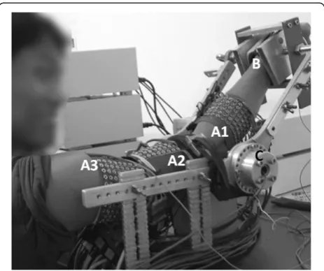
laboratory and consisted in silver-plated and gel-filled eyelets (external diameter of 5 mm) equally spaced by 10 mm in rows (y in the proximal-distal direction) and col-umns (x in the medial-lateral direction). Textile fabric adapts to the geometry of the muscle while maintaining inter-electrode distance and good adhesion to the skin provided by elastic straps. Array 1 (forearm) had 6 rows and a variable number of columns (between 17 and 19) depending on the dimensions of the limb of the subject whereas arrays 2 and 3 (upper arm) consisted of 120 electrodes distributed in 8 rows × 15 columns. About 350 channels were recorded for each subject and were sufficient to cover the muscles of interest.
High Density monopolar signals were recorded si-multaneously by three synchronized amplifiers (EMG-USB- 128 channels, sampling frequency of 2048 Hz, 3dB bandwidth 10–750 Hz, programmable gains of 100, 200, 500, 1000, 2000, 5000 and 10000, LISiN-OT Bioelettro-nica). Power line interference was reduced by using a
“driven right leg” (DRL) circuit [18] and reference elec-trodes were placed at the clavicle, wrist, and shoulder of the same (dominant) side. The force exerted in the four directions of movement (flexion, extension, pronation and supination of the forearm) was measured by two torque transducers (OT Bioelettronica, range 150 N.m, resolution 2.5 mV/V) located at the joints of a mecha-nical brace and aligned with the joint rotational axis. This brace also included an adjustable wrist lock at the end of the bars, in order to avoid hand gripping and wrist flexion/extension efforts (Figure 1). Torque signals were displayed on real time for visual feedback of the exerted force.
Experimental protocol
Twelve healthy male volunteers (age, 28.3 ± 5.5 years; height: 177.8 ± 6.0 cm; body mass: 75.7± 8.7 kg) partici-pated in the experiment. Subjects did not have any his-tory of neuromuscular disorders, pain or regular training of the upper limb. All subjects gave informed consent to participate to the experimental procedure.
Five muscles associated with flexion, extension, prona-tion and supinaprona-tion of the forearm were selected for the study: Biceps and Triceps Brachii in the upper arm and Anconeus, Brachioradialis and Pronator Teres in the forearm. Array 1 (A1) was located on the forearm, with the most proximal electrode row 2 cm below the elbow crease, and was intended for covering the three forearm muscles whose edges were previously drawn over the surface of the skin according to Kendall et al. [19]. The columns of the array laid along the axis oriented from lateral to medial direction in order to cover each selected muscle with at least three columns. Array 2 and array 3 (A2 and A3) were located in the distal and pro-ximal regions of the upper arm, respectively, with their
centers on the location recommended by SENIAM [20]. Previous to the positioning of the electrode array, the skin was shaved and cleaned with abrasive paste. Con-ductive gel (20μl) was inserted in each electrode of the array using a gel dispenser (Multipette Plus, Eppendorf, Germany). Lengths and circumferences of the upper arm and forearm segments were measured for each subject. The length of the ventral side of the upper-arm was measured from the acromion to the fossa cubit whereas the length of its dorsal side was measured from the pos-terior crista of the acromion to the olecranon. The length of the forearm was measured from the medial epicondyle to the apophysis of the radius. Circumfer-ences of the arm segments were measured while con-tracting different muscles: the distal and proximal upper arm circumference were measured over the muscle belly of biceps and triceps respectively and the proximal fore-arm circumference was measured over the muscle belly of the Brachio Radialis (approximately 2 cm below the elbow crease). During the experiment, subjects sat in front of the mechanical brace with the back straight, the elbow joint flexed at 45°, shoulder abducted at 90° (arm in the sagittal plane), and forearm rotated 90°, midway between supination and pronation (Figure 1). Subject’s Maximal Voluntary Contraction (MVC) during flexion, extension, pronation and supination were obtained at the beginning of the experiment as the maximum of three trials for each task. Afterwards, subjects carried out a series of isometric contractions at 10%, 30% and 50% MVC. Contractions were performed in randomized order, each lasting for 10 seconds followed by 2 minutes rest in order to avoid cumulative fatigue. In addition,
subjects were previously trained to maintain the hand and fingers at rest during signal recording.
Detection of low quality signals Features extraction
When recording a large number of physiological signals it is very likely to observe some low quality channels affected by artifacts originated in deformations of the skin under the electrodes, movement of the cables or in bad contacts between each recording electrode and the skin, inducing capacitive couplings and enabling power line interference [21]. Visual inspection of the outliers (channels with low-quality signals) is time-consuming and depends on the expertise of the operators. Thus, it becomes necessary to apply an automatic method to identify such signals (and perform adequate processing if necessary) before any kind of information extraction.
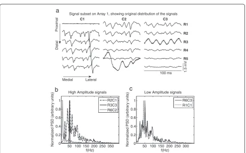
An example of low-quality signals is presented in Figure 2. They are characterized by: a) high-power low
frequency components (R6C2, Figure 2b), b) high power components at power-line harmonics due to high-impedance contacts and stray capacitive couplings (R3C3, Figure 2b), and c) their energy may be much higher or lower than that of neighboring monopolar channels (R1C1, Figure 2c), especially if parallel-fibber muscles are considered. Figure 2c constitutes an especial case where the normalized power spectrum of the sig-nals in R1C1 is similar to that corresponding to a non-artifact; however its amplitude is much lower when compared to its neighbors. Signals R4, R5 and R6 in col-umn C3 have amplitude similar to R1C1, but they are probably located over a region of the limb with lower ac-tivation and cannot be considered as artifacts. Therefore, a detection system should take into account spectral and amplitude features and refer them not only to the bulk of data but also to its neighborhood.
For this purpose, three features for the detection of artifactual signals were defined:
Signal subset on Array 1, showing original distribution of the signals
1.5 mV
Distal
Pro
ximal R1
R2
R3
R4
R5
C1 C2 C3
100 ms
Lateral Medial
50 100 150 200 250 350 0
0.2 0.4 0.6 0.8 1
f(Hz)
Nor
m
aliz
ed PSD (arbitr
a
ry
units)
High Amplitude signals
R2C1 R3C3 R6C2
50 100 150 200 250 300 0
0.2 0.4 0.6 0.8 1
f(Hz)
Nor
m
aliz
ed PSD (arbitr
a
ry
units)
Low Amplitude signals
R6C3 R1C1
a
b
c
Figure 2a) Signal subset recorded in array A1 (forearm) during elbow flexion at 50% MVC.Three columns (C1toC3) and six rows (R1toR6) are shown. Different kinds of artifacts are observed in C1R1, C2R6, and C3R3. It is also possible to observe that the energy of the signals changes in both x and y directions. Normalized Power Spectral Density for different signals are displayed at the bottom. Each spectrum was normalized with respect to its peak value. Artifactual channels can present higher or lower amplitude when compared to neighbor channels.
1. Relative power of low frequency componentsPl/t, from 0 to 12 Hz
2. Relative power of power-line componentsPline/t
corresponding to 50Hz and its first four harmonics, and 3. Signal power calculated from the root mean square
(RMS) of the signal
The Power Spectral Density of the signal was esti-mated with the FFT in non-overlapping signal epochs of 500 ms. Features (Pl/t, Pline/t and RMS) were computed for each channel as the mean of the values obtained from six epochs over segments of 3s where the exerted force remained constant.
Automatic algorithm for artifact removal
An expert system based on thresholds associated with the three features described previously was designed.
The algorithm was applied to a signals set, S, com-posed by signalssi,jrecorded in the rows (i) and columns (j) of a given electrode array A1 to A3 (i=[1,2,. . .,6] and j=[1,2,. . .,17] or j=[1,2,. . .,19]for array A1 depending on the size of the forearm of the subject, and i=[1,2,. . .,8] and j=[1,2,. . .,15] for arrays A2 and A3 in the upper-arm). A schematic of the decision algorithm is presented in Figure 3.
Thresholdsthreshl/t,threshline/tandthreshrmswere calcu-lated from a subset of S composed of signals called refer-ence (ref)that satisfied the following two conditions:
ref¼ abs Pl
t ref
ð Þ median Pl t S ð Þ
0 B @
1 C A 0
B @
1 C
A<1:5IQR Pl
t S ð Þ
0 B @
1 C A
abs Pline t
ref
ð Þ median Pline t
S ð Þ
0 B @
1 C A 0
B @
1 C
A<1:5IQR Pline
t S ð Þ
0 B @
1 C A 8
> > > > > > > > < > > > > > > > > :
ð1Þ
where IQR represents the Interquartile Range. The median was chosen instead of the mean because of its lower sensi-tivity to outliers since it considers the highest breakpoint (50%), that is, the smallest percentage of outliers that can cause an estimator to take arbitrary large values [22].
The thresholds were calculated as following:
threshl
t¼k1 median Pltð Þref
þ1:5IQR Pl tð Þref
ð2Þ
where the constant k1was subjected to an optimization criterion in order to improve the performance of the de-tection method as it is explained in the next section.
threshline
t ¼kline median Plinetð Þref
þ1:5IQR Pline
t ð Þref
h i
ð3Þ
where the constant kline was subjected to a sensitivity analysis (see Table 1 , section Results) and set to 2.5, as a tradeoff between the capacity of threshline/t to identify the highest proportion of signals presenting power-line harmonics and the capacity to correctly identify such signals avoiding the misdetection of good-quality signals. In any case, threshline/t was always constrained to 0.85, that is, signals presenting more than 85% of the signal power in the bands related to power-line harmonics were considered as artifacts.
threshrms¼ min μpa;μpb;μpc
n o
þk2max stdpa;stdpb;stdpc
ð4Þ
Figure 3Schematics of the algorithm for the detection of low quality signals.The symbols (>) or (<) represent the cases where the feature was expected to be higher or lower than the specified threshold in order to determine if a given signal was labeled as artifact.
Table 1 Sensitivity analysis for constantKlinefor the detection of power-line artifacts
kline(2.5) 1 2 3 5 7
Acc 99,74 99,79 99,79 99,74 99,79
S 83,33 83,33 83,33 75,00 75,00
SP 99,83 99,87 99,87 99,87 99,91
P 71,43 76,92 76,92 75,00 81,82
klinein Eq.3was chosen as 2.5 (presented in parenthesis). Increasing values of klinereduced the sensitivity (S) of the thresholdthreshline/t, whereas decreasing
values decreased the precision (P). Variations in these two indexes affected the Accuracy (Acc) and the Specificity (SP).kline= 2.5 is a good compromise
where μ and std are the average and standard devi-ation, respectively, of the RMS of the following three neighbor-pairs in the proximity of a given channel si,j: pa= [RMSi−1,j,RMSi+ 1,j] in the longitudinal direction, and pb= [RMSi−1,j−1,RMSi+ 1,j+ 1] and pc= [RMSi+ 1,j−1, RMSi−1,j+ 1] in the diagonal directions. This third condition
distinguished low amplitude signals corresponding to inner-vations zones or non- active regions (for example R4C3, R5C3 and R6C3 in Figure 2) from isolated low amplitude signals (for example R1C1 in Figure 2) that were considered as artifacts. Hence, the threshold in Eq. 4 takes into account the spatial direction of propagation of Motor Unit Action Potentials. Finally, the constant k2 in Eq. 4 was tuned in order to improve the performance of the method as it is explained in next section.
Training and validation
Constant values ofk1andk2on eq. 2 and eq. 4, allowed to increase the performance of the detection method, especially its sensitivity (or the capacity of the method to identify the highest proportion of low-quality signals) and the precision (or the capacity to correctly identify low-quality signals avoiding the misdetection of good signals as low-quality). Thus, the performance of the method was measured in terms of Sensitivity (S), Specificity (SP), Precision (P) and Accuracy (Acc) as [23]:
S¼ TP
TPþFN⋅SP¼ TN TNþFPP
¼ TP
TPþFP⋅Acc¼
TPþTN
TPþFPþTNþFN ð5Þ
where TP and TN is the number of channels correctly identified as low and good-quality signals respectively, FN is the number of low-quality signals not identified by the algorithm and FP is the number of good-quality signals identified as low-quality.
Signals were visually classified as low-quality or not by three experts based on the observation of similarity be-tween different channels and on the examination of baseline fluctuations or periodicity patterns (related to movement artifacts and power-line interference respect-ively, see Figure 2a as an example). Two databases for training and validation were obtained, each composed of 20 signal sets Sselected from different contractions, ef-fort levels and arrays 1 to 3. Fleiss’Kappa index [24] was used to measure agreement between experts, scoring 82.63% and 86.19% for the training and validation data-bases respectively and indicating an “almost perfect agreement”. The information of the three experts was combined by obtaining the majority vote in each case (i.e. the statistical mode of the three opinions) in order to
obtain a binary classification-label as artifact/non artifacts for each single-channel in the setS.
Optimal values for k1 and k2were tuned according to the following criteria: 1) by Receiver Operating Charac-teristic (ROC) curves (S vs. 1-SP), widely used in signal detection theory and clinical diagnostics [25] and, 2) by Precision-Recall representations (P vs. SP), which are commonly used in machine learning [26]. Both methods assessed the accuracy of the prediction (or outcome) of the described method based on its Sensitivity, Specificity and Precision. The optimal classifier was found as a tra-deoff between hit rates and false alarm rates. In the first case the optimal can be found as the minimum distance between the curve (S vs. 1-SP) and the point [0, 1], and in the second case, as the minimum distance between curve (P vs. SP) and the point [1, 1].
Segmentation of HD-EMG maps
Areas corresponding to electrodes lying over an active region of a muscle or a set of muscles can change be-tween subjects. Therefore, it was useful to extract a delimited region related to each muscle of interest before averaging between subjects, in order to finally obtain a general activation map for the different tasks. Thus, an algorithm for the segmentation of active regions was pro-posed in this study. An activation map Iin the 2D space was calculated from HD-EMG signals as:
Ii;j¼ 1 M
XM
m¼1
1 N
XN
n¼1
s2i;jð Þn !
¼ 1
M XM
m¼1
RMS si;j ð6Þ
wheresis an EMG signal in the channel located at the position i, j of the 2D array (as explained before), N is the total number of samples in an epoch of 500 ms and the RMS value was averaged in M=6 non overlapped epochs corresponding to three seconds of signal. Prior to the calculation of RMS, the signals were filtered be-tween 12 and 350 Hz with a 4th order Butterworth filter in forward and backward direction in order to correct for phase distortion following SENIAM recommenda-tions for the processing of surface EMG signals [27]. RMS values corresponding to signals previously identi-fied as artifacts were replaced by triangle-based cubic interpolation based on Delaunay Triangulation for sur-face fitting proposed in [28].
The activation map was segmented by applying an h-dome transformDh(I)over the image I, as proposed by L. Vincent in [17]. Mathematically, the transformation is defined as:
Dhð Þ ¼I IρIð Þ ¼J IρIðIhÞ ð7Þ
where the operator ρI stand for morphological recon-struction [29], and J is derived from I by subtracting a constant value h. This transformation preserved all the domes above the height h, including those that contain various local maxima. In the case of activation maps, such local maxima could correspond to local variations of the amplitude of the 2D maps due to distinct contact impedances in the various electrodes. Additionally, a morphological opening (γ) was applied to the resulting image Dhin order to avoid the segmentation of isolated peaks, small in area, and which corresponded to pixels with an amplitude slightly higher than that of the sur-rounding channels. This was the case in“flat”maps (par-ticularly at low-effort levels) where the activation is mainly reflected on the synergistic muscles with levels comparable to background noise and where only mar-ginal activation can be observed in antagonist muscles. Therefore, the final segmented image D’h was obtained as:
D0h¼γð Þ ¼Dh Dh∘b¼ðDh⊖bÞ⊕b ð8Þ
where b, the structuring element, is a disc of radius 1 and ⊖and ⊕are the operators for dilation and erosion respectively [29].
Average HD-EMG maps
Average maps for the 12 subjects who participated in the study were obtained by averaging individual segmen-ted maps, in order to obtain useful information relasegmen-ted to muscle co-activation pattern in terms of intensity values and its spatial distribution during different kind of tasks and levels of effort. Considering that upper-limb dimensions, specifically circumference and length, are different for every subject, it was necessary to normalize and interpolate the image in the 2-D space so that results could be comparable among subjects allowing the calculation of an average map for the population. In the case of arrays A2 and A3 (biceps and triceps), the zero of the coordinate system was defined to correspond to landmarks defined by SEMIAM project [20]. In the case of forearm muscles, the origin of the x-axislaid in the intersection of the line connecting the origin and in-sertion of each muscle (Anconeus, Brachioradialis or Pronator Teres) and an arch traced around the forearm, 2 cm below the elbow crease which in turn was the zero of they-axis.Values in thexdimension were normalized
with respect to the circumferences of the different arm segments: proximal forearm for array A1, distal upper-arm for array A2 and proximal upper-upper-arm for array A3, and values in they dimension were normalized with re-spect to the muscle length as described in the protocol description. In order to obtain individual maps with the same (i, j) coordinates for the calculation of population’s average map, RMS values in the 2-D space were re-sampled by cubic splines interpolation in the x and y directions, considering units relative to the total length and total circumference of the arm segment as explained in the previous paragraph.
Intensity of the maps was parameterized by the aver-age RMS value (RMSav-HD) for the segmented area. In
addition, spatial distribution of the maps was parameter-ized according to the median of its projection over thex and yaxes, that is, x=μxor y=μywhere such projection was divided into two regions of equal area, as following:
Xμdim
k¼1
Qdimk ¼ XM
k¼μdim
Qdimk ¼ 1 2
XM
k¼1
Qdimk
whereQdim
k ¼ max D
0
h;dim
ð9Þ
where Qkdim is the value of the projection of the max-imum of the segmented mapD’hat thekthcoordinate along the dimensiondim= x or dim=yand μdimcorresponds to the median of the projectionQkdim.The median of the pro-jections permitted to evaluate spatial shifts along thexand y-axes of the maps, both of them associated with changes in effort levels or even with different tasks.
On the other hand, data similar to that obtained with bipolar electrodes was extracted by selecting two mono-polar channels for each muscle in the 2D arrays: the first electrode corresponded to the one located at the origin of the coordinate system (i.e. reference in SENIAM re-commendations [20]) as described previously for each muscle, and the second one was located 10 mm apart in the direction of the muscular fibers. For each muscle, a single differential signal was obtained from these two channels and its corresponding RMSav-bip value was
cal-culated at the same time-interval as in the case of HD-EMG maps. The variables RMSav-bip and RMSav-HD
(from bipolar or HD-EMG configurations) were used in the identification of tasks and their performances were compared as later explained.
Statistical analysis
related to the signal power, and μx and μy associated
with the spatial distribution of the maps.
Factors considered in the statistical analysis were: 1) the type of electrode (bipolar or HD-EMG), 2) The type of task, that is, flexion, extension, supination and prona-tion, and contraction level (10%, 30% and 50% MVC), and 3) Muscle (i.e. biceps, triceps, brachioradialis, anconeus and pronator teres).
Differences between RMSav-bip and RMSav-HD were
evaluated with the non-parametric Friedman test in two-way layout. In order to avoid differences between the type of recording (bipolar and monopolar), both vari-ables in each muscle were normalized with respect to the mean value obtained in all tasks and contraction levels. Data corresponding to different tasks and effort levels were pooled together by considering blocks with replication of cells of the factor muscle according to the procedure described in [30] and implemented in the statistical toolbox of MATLABW.
On the other hand, the capacity of the extracted vari-ables (RMSav-bip or RMSav-HD) for the identification of
tasks and/or effort levels was evaluated by classifying the data into different groups based on linear discriminant analysis [31] and cross-validation with the Leaving One Out Method [32]. Data was classified into four or twelve groups corresponding to type of task or to type of task and effort level respectively. In the former case, samples corresponding to the three levels of effort were pooled together for each type of task. The overall classification performance was obtained in terms of Accuracy, Sensi-tivity, Specificity and Precision as described in [23] and (Eq. 5). For this analysis TP were data samples well clas-sified into any of the classes, FN corresponded to the number of missing samples in any of the classes, that is, samples belonging to a given class but that were classi-fied in another, TN were not misclassiclassi-fied samples, and FP were samples misclassified in any of the classes.
In addition, changes in the spatial distribution of the maps due to type of task and effort level were analyzed with a non-parametric repeated measures design based on the Friedman test. In this case, var-iations of the variables μx and μy were evaluated in 12 different measures corresponding to four types of task by three levels of effort each. A Bonferroni cor-rection was applied in order to take into account the multiple comparisons.
Finally, pair-wise comparisons were analyzed trough non-parametric Wilcoxon signed rank test.
Statistical significance was set to p=0.05. In the Friedman test,χ2statistics was considered significant for
χ2
(d.o.f=1)> 3.84 for one degree of freedom (d.o.f = 2 types of electrode −1) and for χ2 (d.o.f=11)> 27.28 for eleven degrees of freedom (d.o.f=12 measures −1) after the Bonferroni correction.
Results
Detection of low-quality signals
Sensitivity analysis in the training database for constant kline in Eq. 3 is presented in Table 1. Higher values of klineincreased the number of TP and FP affecting both, the sensitivity and the precision of the detection. As it can be observed on Table 1, kline between 2 and 3 is a good compromise between sensitivity and precision and it can be confirmed from the accuracy and specificity, where the highest values were obtained. For values lower than 2, precision decreases whereas for values higher than 3, sensitivity decreases.
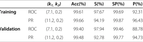
Performance indexes for the detection of artifacts in the training and validation databases using ROC and PR are shown in Table 2. Although results were similar when comparing both criteria, the precision was higher for the PR approach at the expense of slightly lower sensitivity be-cause of the introduction of a number of FN. The sensitiv-ity was higher when considering the ROC criterion but this led to an increase in the number of FP (as compared to PR). The specificity was always very high (above 99%) because the number of non-artifact signals is much higher than the number of low-quality signals. A sensitivity ana-lysis for k1 and k2 in the training database is presented in Figure 4. Different values ofk2produced the same sensi-tivity for increasing values ofk1whereas the precision var-ied at high values of k1 (because of the inclusion of FP). Precision and sensitivity increased and decreased respect-ively for increasing values ofk1. The values adopted fork1 and k2 in this work represent a good tradeoff between sensitivity, specificity and precision.
Although high Sensitivity (S) and Specificity (SP) were desired, a lower number of FP became important when considering the next step of the analysis where RMS values of artifacts were interpolated from neighbor chan-nels. If too many channels in the neighborhood were wrongly labeled as“artifacts”(i.e. too many FP), then the interpolation process was not possible. Because of the lower Precision of the algorithm with the ROC criterion (Table 2), constants k1 and k2 were finally selected ac-cording to optimization results obtained by Precision-Recall.
Table 2 Optimum values ofk1andk2(Eq.2 and Eq.4) and their performance indexes
(k1,k2) Acc(%) S(%) SP(%) P(%)
Training ROC (7.1, 0.2) 99.61 97.67 99.69 92.31
PR (11.2, 0.2) 99.66 94.19 99.87 96.43
Validation ROC (7.1, 0.2) 99.40 97.94 99.46 88.78
PR (11.2, 0.2) 99.48 92.78 99.77 94.73
Performance measures for combinations of k1and k2: Accuracy (A), Sensitivity
On the other hand, the algorithm for artifact detection had low computational complexity. The execution time of the algorithm, (mean and standard deviation for joint training and validation databases), was 201.2±12.85 ms, [min: 187.5 ms, max 234.4 ms] per signal set on a 2.13
GHz IntelW Core2™ processor. Each set had a total duration of 3s and was composed by a different number of channels between 109 and 120 channels.
Segmentation
An example of the surface obtained after the triangle-based cubic interpolation of channels identified as arti-facts can be observed in Figure 5. Additionally, an ex-ample of the segmentation of different maps obtained for flexion, extension, pronation and supination in the five muscles is presented in Figure 6. The shape of the segmented area depended on the intensity of the peaks.
The segmentation produced intensity maps for each muscle and subject, and allowed the calculation of aver-age HD-EMG maps representative for the 12 subjects in the study.
Bipolarvs.High-density EMG signals
Significant differences were observed for the two-way Friedman test between RMSav-bip and RMSav-HD using
the factor muscle as blocking factor (χ2 [1] = 16.55, p<0.001). Thus, significant differences were observed when characterizing the different tasks and effort levels with information extracted from one or the other type of sensor.
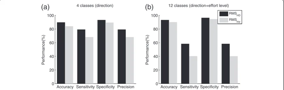
Results for the overall classification into four or twelve groups are presented in Figure 7 for the variables RMSav-bip
and RMSav-HD.
Average HD-EMG Maps
Average activation maps for the 12 subjects at 10, 30 and 50% MVC for each of the four tasks under
stu-6
8
10
12
14
85
90
95
100
k
1Performance(%)
Acc
S
P
k2=0.1k2=0.2 k2=0.3
Figure 4Sensitivity analysis fork1andk2in the training
database.Constantk1is represented along the x-axis. Curves
(in shades of gray) are shown fork2. Higher values ofk1increased
P (in dot lines) but decreased S (in solid lines). Acc (dash lines) remained almost constant for different values ofk1andk2. Optimal
values fork1were found as a compromise between S and SP and
the obtained ranges are highlighted in gray-shadowed areas. Performance indexes corresponding to the selectedk2=0.2 are
shown in squares.
0 2
4 6
8
0 2 4 6 8 0.1 0.15 0.2
midle to lateral
proximal to distal
RMS (mV)
Activation map Artifacts
0 2
4 6
8
0 2 4 6 8 0.1 0.15 0.2
midle to lateral
proximal to distal
RMS (mV)
Activation map Interpolated channel
dy were obtained by averaging the individual maps of each subject. Results on average maps at 50% MVC are displayed in Figure 8. It is possible to observe different muscle co-activation patterns resulting from muscle in-teractions when performing a given task. Variability between subjects was measured through the standard deviation divided by the intensity for each pixel of the average map. Results are presented in Table 3.
In addition to the average maps at 50% MVC, their
projections Qkx at 10%, 30% and 50% MVC for the
two most active muscles in each type of task are presented in Figure 9. Each projection was normal-ized with respect to the maximum value reached at 50% MVC in order to observe changes of the inten-sity as a function of effort level and to compare
among muscles and/or tasks. Changes observed are summarized as following:
Flexion: Intensity decreased with decreasing levels of
effort (from 50 to 10% MVC) in Biceps and Brachioradialis (p<0.0005), preserving a similar
proportion in both muscles (Figure9a).
Extension: Intensity in Triceps decayed
proportionally from 50% to 10% MVC (p<0.0005), but not in the Anconeus, where the maximum of the distribution was significantly different between 10% and 30% MVC (p<0.009) but not between 30%
and 50% MVC (Figure9b).
Supination: Intensity decreased from 50 to 10%
MVC in Biceps and Anconeus (p<0.0005) but not in
Figure 6Example of segmentation of HD- EMG Maps from the right arm of subject 5: Triceps (top left), Biceps (top right), Brachio Radialis (bottom left), Anconeus (bottom middle), and Pronator Teres (bottom right).Maps corresponding to 50% MVC in exercises associated with the main function of each muscle are presented. Final segmented regions are presented with crosses. Regions limited by dash lines were also segmented and considered as belonging to neighboring muscles and were not taken into account to obtain the average map for the 12 subjects.
Accuracy Sensitivity Specificity Precision 0
20 40 60 80 100
Performance(%)
12 classes (direction+effort level)
(b)
Accuracy Sensitivity Specificity Precision 0
20 40 60 80 100
Performance(%)
4 classes (direction)
(a)
RMS HD RMS
bip
Figure 7Classification performance using the feature RMSav-HD(in black) extracted from HD-EMG maps or RMSav-bip(in gray) extracted
the same proportion in both muscles. Changes in the activation of the Anconeus were proportionally higher at 10% and 30% MVC when compared to changes in biceps, (p<0.003), although the former continued being the most active muscle in the
contraction (Figure9c).
Pronation: Intensity levels in Pronator Teres and
Anconeus decreased similarly from 50 to 10% MVC. However, the normalized levels for Anconeus at 10% MVC were higher than those for Pronator Teres
(p<0.001) showing that the contribution of the former was higher at lower levels of contraction.
(Figure9d).
The identification of movement intention by muscle co-activation is usual in pattern recognition approaches [33]. Although such co-activation pattern has already been assessed with bipolar electrodes, performance of the identification of tasks and even of the intended effort level were improved when considering HD-EMG maps
). U. A( si x a l at si D ot l a mi x or P e ht ni e c n at si D Triceps
d)
Pronation, 50% MVC-0.2 -0.1 0 0.1 -0.15 -0.1 -0.05 0 0.05 0.1 Biceps In te n s ity (d B )
-0.2 -0.1 0 0.1 0.2 -0.05 0 0.05 0.1 0.15 0.2 Brachio Radialis
-0.1 0 0.1 0.1
0.15
0.2
0.25
Anconeo
Distance in the Middle to Lateral axis (A.U.) -0.05 0 0.05 0.1 0.15
Pronator Teres In te n s it y ( d B )
-0.05 0 0.05 0.1
-30 -25 -20 -15 -10 -5 -40 -35 -30 -25 -20 -15 -10 ). U. A( si x a l at si D ot l a mi x or P e ht ni e c n at si D
a)
Flexion, 50% MVCTriceps
-0.2 -0.1 0 0.1 -0.15 -0.1 -0.05 0 0.05 0.1 Biceps In te n s it y ( d B )
-0.2 -0.1 0 0.1 0.2 -0.05 0 0.05 0.1 0.15 0.2 -30 -25 -20 -15 -10 -5 Brachio Radialis
-0.1 0 0.1 0.1
0.15
0.2
0.25
Anconeo
Distance in the Middle to Lateral axis (A.U.) -0.05 0 0.05 0.1 0.15
Pronator Teres In te n s ity (d B )
-0.05 0 0.05 0.1 -40
-35 -30 -25 -20 -15 -10 ). U. A( si x a l at si D ot l a mi x or P e ht ni e c n at si D
b)
Extension, 50% MVCTriceps
-0.2 -0.1 0 0.1 -0.15 -0.1 -0.05 0 0.05 0.1 Biceps In te n s it y ( dB )
-0.2 -0.1 0 0.1 0.2 -0.05 0 0.05 0.1 0.15 0.2 -30 -25 -20 -15 -10 -5 Brachio Radialis
-0.1 0 0.1 0.1
0.15
0.2
0.25
Anconeo
Distance in the Middle to Lateral axis (A.U.)-0.05 0 0.05 0.1 0.15
Pronator Teres In te n s it y ( d B )
-0.05 0 0.05 0.1 -40
-35 -30 -25 -20 -15 -10 ). U. A( si x a l at si D ot l a mi x or P e ht ni e c n at si D
c)
Supination, 50% MVCTriceps
-0.2 -0.1 0 0.1 -0.15 -0.1 -0.05 0 0.05 0.1 Biceps In te n s it y (d B )
-0.2 -0.1 0 0.1 0.2 -0.05 0 0.05 0.1 0.15 0.2 -30 -25 -20 -15 -10 -5 Brachio Radialis
-0.1 0 0.1 0.1
0.15
0.2
0.25
Anconeo
Distance in the Middle to Lateral axis (A.U.) -0.05 0 0.05 0.1 0.15
Pronator Teres In te n s it y ( d B )
-0.05 0 0.05 0.1-40
-35 -30 -25 -20 -15 -10
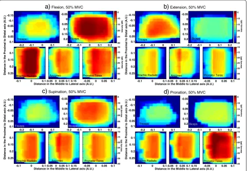
Figure 8Average HD-EMG maps across subjects in the five assessed muscles: Triceps (top left), Biceps (top right), Brachioradialis (bottom left), Anconeus (bottom middle) and Pronator Teres (bottom right).Maps are displayed in dB. The color scale for biceps and triceps is presented at the top of each figure and the color scale for brachioradialis, anconeus and pronator teres is presented at the bottom.
a) Flexion at 50% MVC,b) Extension at 50% MVC,c) Supination at 50% MVC.d) Pronation at 50% MVC.
Table 3 Variability between the 12 individual maps associated with the average HD-EMG maps
10% 30% 50%
Biceps (mean, [min max]) 0.085, [0.07, 0.11] 0.18, [0.16, 0.2] 0.29, [0.23, 0.39]
Triceps (mean, [min max]) 0.13, [0.084, 0.23] 0.15, [0.089, 0.2] 0.24, [0.11, 0.36]
Brachio Radialis (mean, [min max]) 0.14, [0.063, 0.25] 0.16, [0.13, 0.21] 0.23, [0.17, 0.26]
Anconeus (mean, [min max]) 0.13, [0.11, 0.14] 0.18, [0.12, 0.22] 0.2, [0.15, 0.23]
Pronator Teres (mean, [min max]) 0.12, [0.063, 0.2] 0.16, [0.11, 0.2] 0.22, [0.15, 0.29]
-0.2 -0.1 0 0.1 0.2 0.3 0
0.2 0.4 0.6 0.8 1
)
sti
n
u
yr
ar
ti
br
a(
S
M
R
d
e
zil
a
mr
o
N
Distance in the x axis (arbitrary units) Biceps [0.056 mV]
a) Flexion
-0.2 -0.1 0 0.1
0 0.2 0.4 0.6 0.8
1Brachio Radialis [0.031 mV]
50% MVC 30% MVC 10% MVC
-0.40 -0.3 -0.2 -0.1 0 0.1 0.2 0.2
0.4 0.6 0.8 1
)
sti
n
u
yr
ar
ti
br
a(
S
M
R
d
e
zil
a
mr
o
N
Distance in the x axis (arbitrary units) Triceps [0.032 mV]
b)
Extension-0.1 -0.05 0 0.05 0.1 0.15 0.2
0 0.2 0.4 0.6 0.8 1
Anconeus [0.01 mV] 50% MVC 30% MVC 10% MVC
-0.2 -0.1 0 0.1 0.2 0.3
0 0.2 0.4 0.6 0.8 1
)
sti
n
u
yr
ar
ti
br
a(
S
M
R
d
e
zil
a
mr
o
N
Distance in the x axis (arbitrary units) Biceps [0.031 mV]
c) Supination
-0.1 -0.05 0 0.05 0.1 0.15 0.2
0 0.2 0.4 0.6 0.8 1
Anconeus
[0.014 mV] 50% MVC 30% MVC 10% MVC
-0.1 -0.05 0 0.05 0.1 0.15
0 0.2 0.4 0.6 0.8 1
)
sti
n
u
yr
ar
ti
br
a(
S
M
R
d
e
zil
a
mr
o
N
Distance in the x axis (arbitrary units) Pronator Teres [0.028 mV]
d) Pronation
-0.1 -0.05 0 0.05 0.1 0.15 0.2
0 0.2 0.4 0.6 0.8 1
Anconeus [0.013 mV] 50% MVC 30% MVC 10% MVC
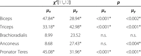
from the upper-arm and forearm (see Figure 7). Add-itionally, differences in the co-activation of muscles were also reflected in the spatial distribution of the maps. Results for the repeated measures Friedman test for the spatial distribution variables μx and μy extracted from HD-EMG maps are presented in Table 4. It is possible to observe that the obtained χ2 values were significant for four of the five analyzed muscles confirming possible changes in the spatial distribution with different tasks and/or effort levels.
Furthermore, pair-wise comparisons between spatial-distribution variables obtained for different effort levels of the same task on a given muscle in Figure 9 were assessed by applying a Wilcoxon signed rank test to the medians. For example, μx in the Biceps, shifted to the
left with increasing levels of contraction during flexion (p<0.02) and during supination (p<0.05). Such shifts were likely due to differences in the activation of the two heads of this muscle. Additionally, significant shifts were also found for the Pronator Teres during pronation (p<0.05).
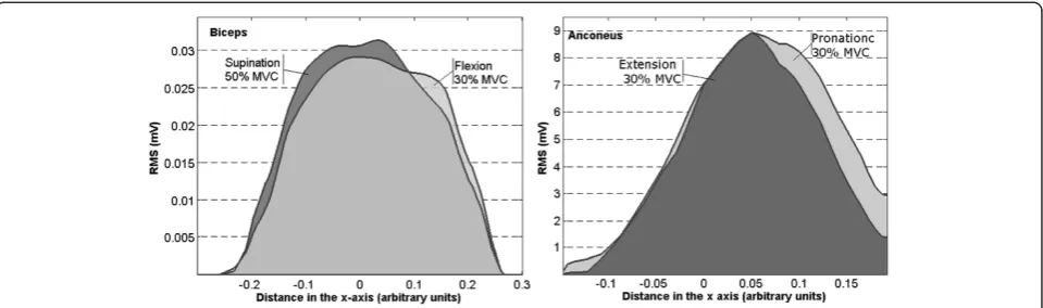
Finally, interesting results were obtained when com-paring spatial distributions between different kinds of task for the same muscle. Intensity levels can be very similar, with no significant differences in the absolute maxima of the projections, but differences were found in the spatial distribution along the x-axis. An example is presented for Biceps during supination at 50% MVC and flexion at 30% MVC in Figure 10: The maxima of the pro-jectionsQkxwere not significantly different (p.n.s) but their spatial distribution differed (i.e. different median μx, p<0.04). This effect was also observed in the Anconeus (Figure 10.) when considering an extension and a prona-tion, both at 30% MVC (p<0.05 for the location of μx). Therefore, even when in these two examples the same muscle is active with similar levels of intensity, only the
spatial distribution permitted to observe differences be-tween tasks.
Discussion and conclusions
The main objective of the study was to extract informa-tion from HD-EMG maps that could be associated with four tasks at the elbow joint (forearm pronation and su-pination, and elbow flexion and extension) at different effort levels. This objective has been reached using 2D arrays of electrodes on five muscles in the upper-arm and forearm. It was shown no only that the average sig-nal power extracted from HD-EMG maps may improve the differentiation of tasks and effort levels but also that the spatial distribution of the maps differed between tasks. Variables related with the spatial distribution of the intensity may complement the information provided by the amplitude of the signals in the identification of motion intention. Additionally, average HD-EMG maps for the four types of tasks and for the group of 12 volun-tary subjects were obtained.
Detection of low-quality signals
Due to the high number of sEMG channels, an algo-rithm for the automatic detection of low quality signals was developed. In this study, the artifactual channels were removed and interpolated based on RMS values of neighbor channels in the HD-EMG maps.
As the number of channels affected by artifacts is usu-ally much lower than the number of non- artifact chan-nels, the number of TN is usually high, so the accuracy and especially, the specificity, is in general very high (>99%). In this study, the percentage of low quality sig-nals was between 0 and 13% of the total number of channels of each set in the training database. For this reason, the ROC method, which was intended to com-promise between specificity and sensitivity, provided an overestimated value of the former (the latter was always very high as it was explained above) at the ex-pense of reducing the precision of the algorithm. On the other hand, PR method maximized the sensitivity while preserving the precision. Considering that both, the spe-cificity and the accuracy were always very high, the use of PR was more convenient in our case since we were dealing with offline detection and interpolation of arti-facts. In addition, the accuracy was slightly higher with the PR method. Other applications, especially those intended for online detection, should consider the ROC approach in order to increase the sensitivity as much as possible.
(See figure on previous page.) Figure 9ProjectionsQk
x
from the two most active muscles for each kind of task.Curves are normalized with respect to the maximum intensity reached at 50% MVC (showed with a label in each plot).a)Flexion in Biceps and Brachio Radialis,b)Extension in Triceps and Anconeus.
c)Supination in Biceps and Anconeus, andd)Pronation in Pronator Teres and Anconeus.
Table 4 Results for the repeated measured friedman test for the variablesμxandμyextracted from HD_EMG
χ2
[11,12] p
μx μy μx μy
Biceps 47.84* 28.94* <0.001* <0.002*
Triceps 33.18* 42.98* <0.001* <0.001*
Brachioradialis 8.99 23.52 n.s. n.s.
Anconeus 8.68 27.43* n.s. <0.004*
Pronator Teres 45.08* 31.96* <0.001* <0.001*
The table presents theX2
In addition, the sensitivity analysis for the constants kline, k1 and k2 in Tables 1 and 2 showed that the se-lected values represented a good compromise between the Precision and Sensitivity of the detection.
Different approaches have also been suggested for the detection of low quality signals. In [16], a non-supervised method based on local distance-based outlier factor was proposed for HD-EMG signals recorded from the same muscles and electrodes arrays. That method did not required a training process and successfully detected low-quality signals with an average Accuracy of 91.9%, Sensi-tivity of 96.9% and Specificity of 96.4%. If the latter index is considered (refer toSPin Eq. 5), it is possible that such method was prone to the inclusion of FP, given that the number of TN is always very high as explained before. This condition was not desired in our study because in-tensity values associated with low quality signals were later replaced in the maps based on neighbor channels, and if those were wrongly identified as artifacts (FP), the interpolation for the replacement was not possible. Thus, another method intended to minimize the number of FP while preserving the accuracy of the detection was pro-posed in the present work. Moreover, the method in [16] did not took into account information provided by neigh-bor channels as in the algorithm described here.
A different study by Gronlund et al. in [15] assumed unimodal distribution of the amplitude of the signals and therefore it was not applicable to cases where the multichannel recording involved various regions with different levels of activity (as in Figure 2) or even with no activity at all. The latter corresponded to regions localized far away from the main activation areas or to muscles marginally active during the contraction (an ex-ample can be observed in Figure 6 bottom-left for the signals recorded in array A1-forearm during flexion). In contrast, the algorithm proposed in the present work la-beled a signal as an artifact based on the amplitude in-formation of 6 neighboring channels (Eq. 4), avoiding
general assumptions on the distribution of the potentials recorded in the array as proposed in [15].
Finally, the algorithm reached very high values for the performance indexes in the validation dataset (see Table 2). In addition, the channels identified as artifacts were correctly interpolated from the information of neighboring non-artifact channels even at the edges of the map (see Figure 5), which provided a smooth surface for subsequent stages of the analysis. Therefore, both the proposed methodology and features showed a very good performance for the detection and off-line replacement of low-quality signals.
Segmentation of HD-EMG maps
An automatic algorithm for the segmentation of active zones was proposed. This segmentation allowed the cal-culation of average HD-EMG maps for the population of 12 subjects by determining the ranges of active zones in the x and y axes relative to upper-limb circumference and muscle length respectively, and referred to the elec-trode location recommended for sEMG recording on the analyzed muscles.
Other methods have been previously proposed for the segmentation of activation maps. Particularly Vieira et al. in [9] proposed a method based on watershed for assessing muscle compartmentalization. Such segmenta-tion was aimed at the extracsegmenta-tion of zones associated with local variations in the level of neuromuscular activity in the same muscle and it was successfully applied with this objective on the gastrocnemius. However, we were inter-ested in obtaining activation maps for different muscles, each of them associated with different types of contrac-tions and levels of effort. This purpose required the iso-lation of muscle activity from background in individual maps before their average. Thus, the segmentation algo-rithm had to extract global active regions, even if those were composed by several regional maxima. This last condition would lead to an over-segmentation in terms
Figure 10ProjectionsQk x
of the purpose of our study when using Watershed tech-niques (see Figure 11). On the other hand, h-dome was applicable straightforward without need of previous equalization or transformation of the original image and was not sensitive to regional maxima [28]. For this rea-son the h-dome transformation was preferred in this work.
Furthermore, it is important to note that maps seg-mentation was not the aim of this study neither the de-termination of anatomical muscle regions but was an intermediate step in order to obtain average maps. It is known that potentials’ amplitude diffuses across skin surface, so the actual size of active muscle regions might be overestimated by the segmentation proposed. In spite of this, the segmentation permitted the extraction of surface areas corresponding to different muscles in individual maps and also permitted to focus on the regions of major activation, avoiding other active neigh-boring areas that could be more affected by the activity of nearby muscles (see Figure 6). By averaging individ-ual segmented maps, it was possible to obtain represen-tative HD-EMG maps associated with the activation of
each muscle during the different tasks and effort levels. In this sense, the segmentation worked properly.
Average HD-EMG maps
Variability in the levels of intensity between subjects with respect to the average HD-EMG maps (Table 3) was found to be low enough to consider such maps as representative for the 12 subjects. The obtained differ-ences were higher for higher levels of contraction (be-tween 20% and 29% in the four tasks at 50% MVC) and being less than 12% for contractions at 10% MVC (see Table 3). In the average activation maps depicted in Figure 8, it is possible to observe changes in the activa-tion pattern corresponding to different tasks. Such dif-ferences were confirmed with the classification by LDA shown in Figure 7. Consequently, results concerning the spatial distribution and the levels of intensity from aver-age maps can be considered as globally associated with the muscle function and to the activation pattern of the subjects in the study.
On the other hand, the classification performance was higher for the average power extracted from HD-EMG
columns
ro
w
s
Original Map
5 10 15
1
2
3
4
5
6
7
8
5 10
15
2 4 6 8 0 0.5 1
columns Topographical View
rows
N
o
rm
a
li
z
e
d
R
M
S
(
a
.u
.)
columns
ro
w
s
Watershed Segmentation
5 10 15
1
2
3
4
5
6
7
8 H-dome Segmentation
ro
w
s
columns
5 10 15
1
2
3
4
5
6
7
8
maps (RMSav-HD) than from bipolar electrodes (RMSav-bip)
either for four or twelve classes, especially when consi-dering the precision and sensitivity of the classification. Therefore it is possible to conclude that information extracted from the amplitude of signals recorded in high-dimensional configuration has more power to differentiate between tasks and even effort levels than single bipolar signals. With this respect, a recent study by Tkach et al. [33] based on information extracted from bipolar signals showed that the classification accuracy for the identifica-tion of motor tasks worsens when considering distinct strengths of the same motion. Substantial drops were observed when training and testing the classifier with data of mixed high and low effort levels, obtaining a maximal accuracy of ~80% for the classification into the four tasks described in the present work. In our case, an overall clas-sification accuracy of approximately 90% for 4 motor tasks with mixed data from very-low to medium-high effort levels (10%, 30% and 50% MVC) was obtained. What is more, classification accuracy for 12 classes was also in the order of 90%. However, in both cases the precision and sensitivity were not very high, thus additional data trans-formations or other features are necessary in order to im-prove the identification performance. In this sense, the Friedman test showed that variables related to the spatial distribution of the maps (μxandμy, see Table 4) may also assist in the discrimination between types of tasks and ef-fort levels.
In addition, Tkach et al. also found that classification accuracy dropped when bipolar electrodes shifted by15 mm [33]. Such shifts could be due to relative move-ments between the recording electrodes and the skin or because of errors when positioning the sensors, for ex-ample in different days. Thus another advantage of HD-EMG maps relies on the contact redundancy implied by the recording of a number of signals over a large surface of the muscle, as well as in the possibility of extracting features associated with spatial-changes induced by the central nervous system in the control of the muscles [11]. All of this makes HD-EMG maps more robust to errors introduced by contact artifacts and by the relative location of the electrodes with respect to the origin of the potentials, especially in contractions involving joint movement or sensor repositioning.
When analyzing variables associated with the activa-tion maps for the 12 subjects, it was possible to ob-serve differences in the co-activation pattern of the muscles according to the kind of task and the effort level. For example during flexion at 50% MVC (see Figure 6), the Biceps, and the Brachioradialis were the most active muscles (as expected) but there was also an important activation of the Anconeus and of the Pronator Teres likely to stabilize the elbow joint and to compensate for the supination action of the biceps.
The extension at 50% MVC was mainly produced by the Triceps and the Anconeus but the other two ana-lyzed muscles in the forearm were also active. All selected muscles but Triceps were involved during Su-pination at 50% MVC with similar intensity levels among them. Finally, during Pronation at 50% MVC, naturally the most active muscle was the Pronator Teres but both the Anconeus and the Brachioradialis were also active while the muscles of the upper-arm appeared not to be active during the contraction. Add-itionally, when considering activation patterns for con-tractions at 30% and 10% MVC it was found that the levels of intensity did not decreased proportionally with effort level in all of the muscles, showing changes in the load-sharing of the involved muscles.
Differences in the average maps between 10%, 30% and 50% MVC were not only related to the levels of in-tensity but also to its spatial distribution. It was pos-sible to observe differences in their projection over the x-axis (see Figure 9 and 10 and Table 4) for different effort levels depending on the task. These variations corresponded to shifts in the lateral to medial axis when the level of effort changed from 10% to 50% MVC. Furthermore, similar values of intensity were obtained for different kind of tasks in some muscles and differences were only found in the spatial distribu-tions of the maps.
For all of this, HD-EMG maps instead of single bipolar signals, and variables related to maps intensity and spatial distribution might be useful in applications where identification of movement intention is needed: for ex-ample in robotic-aided therapies focused on the im-provement of muscle coordination where interaction between patient and machine is involved and where the robot has to be able to sense patient’s intention [34]. Additionally, other applications implying proportional control for devices like powered- prostheses or orthoses could benefit from information provided by HD-EMG maps regarding not only the task but also its strength.
Abbreviations
Acc: Accuracy; DRL: Driven Right Leg; EMG: Electromyography; FN: False negatives; FP: False Positives; HD-EMG: High Density Surface
Electromyography; MVC: Maximal Voluntary Contraction; P: Precision; PSD: Power Spectral Density; PR: Precision- Recall representation; RMS: Root Mean Square; ROC: Receiver Operating Characteristics; S: Sensitivity; SP: Specificity; TN: True Negatives; TP: True Positives.
Competing interest
The authors declare that they have no competing interests.
Authors’contributions
Acknowledgements
The experimental part of this work was carried out in the Laboratory for Engineering of the Neuromuscular System (LISiN), Politecnico di Torino, Italy, under the supervision of Prof R. Merletti. This work was partially supported by the MINECO of the Spanish Government (project DPI2011-22680), by the Grant BE-00194 from AGAUR and by the CIDEM (Generalitat de Catalunya) with the project Neurorehab 3E+D (RD08-2-0019). We are grateful to Dr. Roberto Merletti and Dr. Hamid Reza Marateb for reviewing a draft of this paper.
Author details
1
Biomedical Research Networking Center in Bioengineering, Biomaterials and Nanomedicine (CIBER-BBN), Barcelona, Spain.2Biomedical Engineering Research Centre (CREB), Barcelona, Spain.3Barcelona College of Industrial Engineering (EUETIB), Barcelona, Spain.4Department of Automatic Control (ESAII) Universitat Politecnica Catalunya, Barcelona, Spain.
Received: 17 December 2011 Accepted: 29 November 2012 Published: 10 December 2012
References
1. Nishikawa D, Wenwei Y, Yokoi H, Kakazu Y:EMG prosthetic hand controller using real-time learning method.Proc IEEE Int Conf Syst Man Cybern1999,
1:153–158.
2. Dipietro L, Ferraro M, Palazzolo JJ, Krebs HI, Volpe BT, Hogan N:Customized interactive robotic treatment for stroke: EMG-triggered therapy.IEEE Trans Neural Syst Rehabil Eng2005,13(3):325–334.
3. Drost G, Stegeman DF, Schillings ML, Horemans HLD, Janssen HMHA, Massa M,et al:Motor unit characteristics in healthy subjects and those with postpoliomyelitis syndrome: A high-density surface EMG study.Muscle Nerve2004,30(3):269–276.
4. Kleine BU, van Dijk JP, Lapatki BG, Zwarts MJ, Stegeman DF:Using two-dimensional spatial information in decomposition of surface EMG signals.J Electromyogr Kinesiol2007,17(5):535–548.
5. Zwarts MJ, Stegeman DF:Multichannel surface EMG: Basic aspects and clinical utility.Muscle Nerve2003,28(1):1–17.
6. Holobar A, Minetto MA, Botter A, Negro F, Farina D:Experimental analysis of accuracy in the identification of motor unit spike trains from high-density surface EMG.IEEE Trans Neural Syst Rehabil Eng2010,18(3):221–229. 7. Merletti R, Holobar A, Farina D:Analysis of motor units with high-density
surface electromyography.J Electromyogr Kinesiol2008,18(6):879–890. 8. Farina D, Lorrain T, Negro F, Jiang N:High-density EMG E-textile systems
for the control of active prostheses.Proc IEEE Int Conf Eng Med Biol Soc 2010:3591–3593.
9. Vieira TMM, Merletti R, Mesin L:Automatic segmentation of surface EMG images: Improving the estimation of neuromuscular activity.J Biomech 2010,43(11):2149–2158.
10. Tucker K, Falla D, Graven-Nielsen T, Farina D:Electromyographic mapping of the erector spinae muscle with varying load and during sustained contraction.J Electromyogr Kinesiol2009,19(3):373–379.
11. Holtermann A, Roeleveld K, Karlsson JS:Inhomogeneities in muscle activation reveal motor unit recruitment.J Electromyogr Kinesiol2005,
15(2):131–137.
12. Staudenmann D, Kingma I, Daffertshofer A, Stegeman DF, van Dieën JH:
Heterogeneity of muscle activation in relation to force direction: A multi-channel surface electromyography study on the triceps surae muscle.
J Electromyogr Kinesiol2009,19(5):882–895.
13. Merletti R, Aventaggiato M, Botter A, Holobar A, Marateb H, Vieira TMM:
Advances in surface EMG: Recent progress in detection and processing techniques.Crit Rev Biomed Eng2010,38(4):305–345.
14. Merletti R, Botter A, Cescon C, Minetto MA, Vieira TMM:Advances in surface EMG: Recent progress in clinical research applications.Crit Rev Biomed Eng2010,38(4):347–379.
15. Gronlund C, Roeleveld K, Holtermann A, Karlsson JS:On-line signal quality estimation of multichannel surface electromyograms.Med Biol Eng Comput2005,43(3):357–364.
16. Marateb HR, Rojas-Martinez M, Mansourian M, Merletti R, Mananas Villanueva MA:Outlier detection in high-density surface electromyographic signals.Med Biol Eng Comput2012,50(1):79–89.
17. Vincent L:Morphological grayscale reconstruction in image analysis: Applications and efficient algorithms.IEEE Trans Image Process1993,
2(2):176–201.
18. Metting Van Rijn A, Peper A, Grimbergen C:High-quality recording of bioelectric events.Med Biol Eng Comput1990,28(5):389–397.
19. Kendall F, McCreary E, Provance P:Muscles: Testing and Function. 4th edition. Baltimore, Md: Williams & Wilkins; 1993.
20. Freriks B, Hermens HJ:SENIAM9: European Recommendations for Surface ElectroMyoGraphy, Results of the SENIAM Project, ISBN: 90-75452-14-4 (CD-rom). The Netherlands: Roessingh Research and Development; 1999. 21. Clancy EA, Morin EL, Merletti R:Sampling, noise-reduction and amplitude
estimation issues in surface electromyography.J Electromyogr Kinesiol 2002,12(1):1–16.
22. Hampel FR:A general qualitative definition of robustness.Ann Math Stat 1971,42(6):1887–1896.
23. Farina D, Colombo R, Merletti R, Baare Olsen H:Evaluation of intra-muscular EMG signal decomposition algorithms.J Electromyogr Kinesiol 2001,11(3):175–187.
24. Fleiss JL:Measuring nominal scale agreement among many raters.
Psychol Bull1971,76(5):378–382.
25. Fawcett T:An introduction to ROC analysis.Pattern Recog Lett.2006,
27(8):861–874.
26. Landgrebe TC, Paclik P, Duin RP, Bradley AP:Precision-recall operating characteristic (P-ROC) curves in imprecise environments.In Proceedings of 18th International Conference on Pattern Recognition. Los Alamitos, California USA.IEEE Computer Society2006,4:123–127.
27. Hermens H, Freriks B, Disselhorst-Klug C, Rau G:Development of recommendations for sensors and sensor placement procedures.
J Electromyogr Kinesiol2000,10(5):361–374.
28. Bradford Barber C, Dobkin DP, Huhdanpaa H:The quickhull algorithm for convex hulls.ACM Trans Math Softw1996,22(4):469–483.
29. Serra J:Image analysis and mathematical morphology. London: Academic; 1982.
30. Zar JH:Biostatistical analysis. 5th edition. New Jersey: Prentice Hall; 2010. 31. Krzanowski WJ:Principles of multivariate analysis: A user's perspective. New
York: Oxford University Press; 1988.
32. Kearns M, Ron D:Algorithmic stability and sanity-check bounds for leave-one-out cross-validation.Neural Comput1999,11(6):1427–1453.
33. Tkach D, Huang H, Kuiken TA:Study of stability of time-domain features for electromyographic pattern recognition.J Neuroeng Rehabil2010,7:21. 34. Hogan N, Krebs HI, Rohrer B, Palazzolo JJ, Dipietro L, Fasoli SE,et al:
Motions or muscles? some behavioral factors underlying robotic assistance of motor recovery.J Rehabil Res Dev2006,43(5):605–618.
doi:10.1186/1743-0003-9-85
Cite this article as:Rojas-Martínezet al.:High-density surface EMG maps from upper-arm and forearm muscles.Journal of NeuroEngineering and Rehabilitation20129:85.
Submit your next manuscript to BioMed Central and take full advantage of:
• Convenient online submission
• Thorough peer review
• No space constraints or color figure charges
• Immediate publication on acceptance
• Inclusion in PubMed, CAS, Scopus and Google Scholar
• Research which is freely available for redistribution