www.geosci-model-dev.net/10/945/2017/ doi:10.5194/gmd-10-945-2017
© Author(s) 2017. CC Attribution 3.0 License.
A cloud feedback emulator (CFE, version 1.0) for an intermediate
complexity model
David J. Ullman1,aand Andreas Schmittner1
1College of Earth, Ocean, and Atmospheric Sciences, Oregon State University, Corvallis, OR 97331 USA anow at: Northland College, Ashland, WI, USA
Correspondence to:David J. Ullman ([email protected]) Received: 20 August 2016 – Discussion started: 26 September 2016
Revised: 18 January 2017 – Accepted: 27 January 2017 – Published: 23 February 2017
Abstract.The dominant source of inter-model differences in comprehensive global climate models (GCMs) are cloud ra-diative effects on Earth’s energy budget. Intermediate com-plexity models, while able to run more efficiently, often lack cloud feedbacks. Here, we describe and evaluate a method for applying GCM-derived shortwave and longwave cloud feedbacks from 4×CO2 and Last Glacial Maximum
exper-iments to the University of Victoria Earth System Climate Model. The method generally captures the spread in top-of-the-atmosphere radiative feedbacks between the original GCMs, which impacts the magnitude and spatial distribu-tion of surface temperature changes and climate sensitivity. These results suggest that the method is suitable to incorpo-rate multi-model cloud feedback uncertainties in ensemble simulations with a single intermediate complexity model.
1 Introduction
The predominant trade-off in climate modeling is that of sys-tematic complexity vs. computational expense. While com-prehensive global climate models (GCMs) attempt to resolve the complex interactions between Earth systems, their com-putational expense limits the exploration of parametric un-certainty. Conversely, more simplified models, such as Earth system models of intermediate complexity (EMICs), can be employed for large-ensemble analysis of parametric variabil-ity, but their reliance on fixed boundary conditions or gener-alized parameterizations of earth processes may not capture all important feedbacks driving system dynamics.
One of the largest sources of inter-model spread in GCM-based climate projections is the magnitude and direction of
im-of state-im-of-the-art GCMs into an EMIC, thereby creating a computationally less-expensive emulator of more complex models.
2 Methods
2.1 Model description
The UVic Earth System Climate Model (Weaver et al., 2001) is an EMIC with a three-dimensional ocean general circu-lation model coupled to a dynamic–thermodynamic sea ice model, a two-dimensional single-layer energy–moisture bal-ance atmosphere, and a dynamic land (Meissner et al., 2003) and vegetation model (Cox, 2001). Surface wind speeds used in the calculations of air–sea exchange and atmospheric transport of heat and moisture are prescribed in the model, thereby limiting variability in the atmospheric model. The model conserves heat and moisture without the need for a flux correction (Weaver et al., 2001). We employ version 2.9 of UVic (Eby et al., 2013), in which atmospheric heat diffu-sion varies with changes in global-mean surface air temper-ature; this modification has been shown to improve the lati-tudinal temperature gradient for the Last Glacial Maximum when compared with high-latitude proxy data (Fyke and Eby, 2012). All model components have a horizontal grid resolu-tion of 1.8◦latitude by 3.6◦longitude, with 19 vertical levels in the ocean model increasing from 50 m thickness in the sur-face level to 590 m thickness in the deepest grid cell.
The net radiative balance (NETRAD) at the top of the atmosphere (TOA) is the difference between the net short-wave radiation (SWTOA)and the outgoing longwave
radia-tion (OLW):
NETRAD=SWTOA−OLW. (1)
Clouds impact SWTOAthrough prescribed monthly fields of
atmospheric albedo (αatm):
SWTOA=SWin,TOA−SWin,TOA×αatm−SWin,TOA
×(1−αatm)×αsfc×τ2, (2)
cover, vegetation, etc.),αatmis a fixed boundary condition at
monthly resolution to resolve seasonal changes in regional cloud cover. In the control version of UVic,αatmis estimated
with the following relationship: αatm=
f×αplt−αsfc
1−αsfc×τ2
, (3)
where αplt=
SWout,TOA
SWin,TOA
, (4)
αsfc=
SWout,sfc
SWin,sfc
, (5)
where the planetary (αplt)and surface albedo (αsfc)are
calcu-lated using the incoming and outgoing shortwave satellite ob-servational measurements at the surface and top of the atmo-sphere from the Earth Radiation Budget Experiment (ERBE; Barkstrom, 1984; Barkstrom and Smith, 1986; Ramanathan et al., 1989). Thisαatmrelationship is directly derived from
Eq. (2) so as to be internally consistent with the radiative balance relationship from the UVic model. The variable f in Eq. (3) is a constant planetary albedo adjustment factor to account for radiative imbalances that arise in the implemen-tation of the derivedαatm.
The OLW is parameterized in UVic using an empirical relationship (Thompson and Warren, 1982; Weaver et al., 2001) that determines clear-sky OLW as a function of on sur-face relative humidity (RH) and temperature (SAT):
OLW=c00+c01RH+c02RH2
+c10+c11RH+c12RH2
SAT +c20+c21RH+c22RH2
SAT2 +c30+c31RH+c32RH2
SAT3 +1F2xCO2ln
[CO2]t [CO2]o
, (6)
1F2xCO2=5.35 W m
−2 is selected as the radiative forcing
associated with 3.71 W m−2 (IPCC, 2001). The constants
(cxx)are provided by Thompson and Warren (1982). Since this was originally estimated as a clear-sky relationship, the effect of clouds on the OLW radiative balance is not explicitly included.
2.2 CERES update to atmospheric albedo boundary conditions
Because of discontinuities in satellite coverage, missing data, and poor resolution, the Clouds and the Earth’s Radiant En-ergy System (CERES; Wielicki et al., 1996) was launched in late 1999 to better observe the Earth’s radiative balance (Fa-sullo and Trenberth, 2008). The CERES experiment uses an updated satellite architecture and provides higher spatial res-olution observations over a longer time domain (2000–2013 for CERES compared with 1985–1989 for ERBE), thereby providing more robust modern climatology on the impact of clouds on atmospheric albedo (Wielicki et al., 1996). In ad-dition, the duration of the ERBE experiment between 1985 to 1989 spans a somewhat large El Niño event (1987), which may bias the equatorial Pacific toward enhanced cloudiness in the calculation of atmospheric albedo climatology using the ERBE data (Cess et al., 2001).
In this paper, we use the climatology (2000–2013) of CERES surface and top of the atmosphere shortwave fluxes to better estimateαatmboundary conditions in UVic (using
Eq. 3). Under low-light conditions (winter, high-latitudes), satellite-derived estimates of incoming SW are small, which occasionally results in values ofαpltandαsfcthat are greater
than 1. Therefore, we limitαpltandαsfcto values less than 1,
which ensures thatαatmis within appropriate limits.
An ensemble of control simulations was performed using the new CERES-based estimates ofαatmwith varying values
of thef parameter in Eg. (3). From the resulting equilibrium simulations, a value off =0.95 in Eq. (3) was selected in or-der to match 20th century global mean temperature data esti-mates of∼13.9◦C (NOAA, 2016) in a UVic control simula-tion. This final estimate of CERES-basedαatmwas smoothed
and regridded to the UVic grid.
Figure 1 compares the annual-mean values ofαatmas
de-rived from the ERBE and CERES datasets. In the tropics, the ERBE-based estimates ofαatmgenerally match those of the
CERES-based values (Fig. 1). In the high latitudes, however, the ERBE-based αatm values are generally higher than the
CERES-based values. Such differences are likely related to improvement in sampling orbit of the CERES satellite and the associated reduction in zenith angle-dependent biases, which may result in large errors in the top-of-the-atmosphere flux measurements in the ERBE data (Loeb et al., 2009). Furthermore, the use of CERES-based estimates ofαatm
pro-vides an improvement in UVic, particularly at high latitudes.
2.3 Innovations
With the use of CERES-based αatm estimates, the UVic
model now includes an updated effect of clouds on the Earth’s shortwave radiative balance. However, the control UVic model design does not incorporate any change in the shortwave or longwave radiative effect of clouds due to changes in temperature. This lack of cloud feedbacks may significantly limit the ability of UVic to capture global tem-perature in perturbed simulations. Here, we provide a simple method of diagnosing cloud radiative forcings from GCM results of the Coupled Model Intercomparison Project 5 (CMIP5) and Paleoclimate Model Intercomparison Project 3 (PMIP3) archives (Braconnot et al., 2011; Taylor et al., 2012) and incorporate the associated shortwave and long-wave cloud feedbacks into UVic for both 4 times CO2
(4xCO2)and Last Glacial Maximum (LGM) climate
simu-lations. Reanalysis of satellite observations suggests that the range of CMIP5 models present widespread agreement with cloud data, both in spatial extent and vertical distribution, across the historical record (Norris et al., 2016). We have selected model output from seven GCMs: Community Cli-mate System Model version 4 (abbreviated as CCSM), Cen-tre National de Recherches Meteorologiques version CM5 (CNRM), Goddard Institute for Space Sciences Model E2-R (GISS), Institute Pierre Simon Laplace CM5A-LE2-R (IPSL), Model for Interdisciplinary Research on Climate-Earth Sys-tem Model (MIROC), Max Planck Institut model ESM-P (MPI), Meteorological Research Institute model CGCM3 (MRI). These models were chosen because they have results for both 4×CO2and LGM simulations and all of the relevant
variables for calculating shortwave and longwave cloud feed-backs (see below). The following innovations demonstrate how we employ UVic as a cloud feedback emulator (CFE version 1.0; henceforth CFE) of the full GCMs.
2.3.1 Shortwave cloud feedbacks in UVic
Since UVic incorporates the shortwave impact of clouds through atmospheric albedo, we assess the shortwave cloud feedback as the change inαatmdue to the change in
temper-ature in each of the GCM simulations. Albedo anomalies are not mathematically additive; therefore, we first calculateαatm
for each perturbed state (4×CO2, LGM) by adding GCM
anomalies of each of the individual fluxes to the CERES ob-servations:
SWin,TOA,GCM=(SWin,TOA,perturbed−SWin,TOA,control)
+SWin,TOA,CERES, (7)
SWout,TOA,GCM=(SWout,TOA,perturbed−SWout,TOA,control)
+SWout,TOA,CERES, (8)
SWin,sfc,GCM=(SWin,sfc,perturbed−SWin,sfc,control)
+SWin,sfc,CERES, (9)
Figure 1.Comparison of annual-averaged atmospheric albedo (αatm)as calculated using Eq. (3) and the climatology of ERBE (left) and CERES (right) data.
+SWout,sfc,CERES. (10)
For each of the variables, we have calculated a 12-month climatology (separate averaging for each month) that is as-sessed over the final 10 years of the 150 year transient 4×CO2simulations, the final 100 years of the LGM
equilib-rium simulations, and the final 100 years of the equilibequilib-rium control simulations. The anomaly perturbed values of each of the shortwave fluxes (Eqs. 7–10) are then used to calculate an αatm,perturbed for each of the perturbed GCM simulations
us-ing Eqs. (3)–(5).
Again, because albedo values are not additive, we calcu-late the albedo anomaly as the ratio of the atmospheric albedo of the GCM perturbed state to CERES-derived atmospheric albedo. Therefore, theαatmfeedback (αatmFB) is this albedo
anomaly divided by the change in temperature: αatmFB=
αatm,perturbedαatm,CERES−1
SATperturbed−SATcontrol
. (11)
The subtraction of 1 in the numerator is necessary such that when there is no change inαatm(αatm,perturbed=αatm,CERES),
then there is no atmospheric albedo feedback. Thisαatm
feed-back is calculated as a 12-month climatology at each grid cell of the seven GCMs that are sampled in this analysis (Figs. 2, 3). Positive (negative) values for this atmospheric albedo feedback indicate a negative (positive) shortwave cloud feed-back since increases in temperature cause an increase (de-crease) in atmospheric albedo, which cools (warms) the sur-face. The magnitude of these atmospheric albedo feedbacks varies considerably among the GCMs and between perturbed climate states (4×CO2vs. LGM), which is consistent with
the large spread in cloud shortwave feedbacks found in pre-vious studies (Tomassini et al., 2013; Vial et al., 2013). For example, GISS-E2-R shows a strongly positive atmospheric albedo feedback from the 4×CO2 results, whereas
IPSL-CM5A-LR generally shows a strongly negative atmospheric albedo feedback, particularly in the tropics (Fig. 2).
The innovation to UVic is the application of these GCM-diagnosedαatmfeedbacks to the shortwave radiative balance.
First, we calculate a SAT climatology from a long-term con-trol simulation of UVic that usesαatm,CERES as the control
atmospheric albedo. Then at each time step (t) of a model simulation, we calculate the difference in surface air tem-perature from this control monthly climatology, and perturb atmosphere albedo at each grid cell using the GCM-derived αatmFB of Eq. (11):
αatm(t )= [αatmFB×[SAT(t )−SATctl]+1]
×αatm,CERES. (12)
The above calculation is done at every time step and each grid cell, allowing for spatially and monthly specific atmospheric albedo feedbacks as diagnosed from the GCMs.
2.3.2 Longwave cloud feedbacks in UVic
Because UVic lacks a longwave cloud feedback in the cal-culation of OLW, we provide an additional term to Eq. (6), which now includes the OLW due to changes in the cloud longwave effect in the GCM simulations. First, we diagnose the outgoing longwave radiation at the top of the atmosphere from the GCM output:
OLWcloud=OLWtotal−OLWclear sky. (13)
The outgoing longwave cloud feedback is therefore the cloud longwave forcing anomaly divided by temperature anomaly: OLWcloudFB=
OLWcloud,perturbed−OLWcloud,control
SATperturbed−SATcontrol
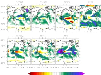
Figure 2.Maps of annual-mean atmospheric albedo feedback term (αatmFB), as calculated using Eq. (11) and the 4×CO2results of the seven CMIP5 models discussed in the text. Units are albedo fraction change per◦C.
states (Figs. 4, 5). Again, OLWcloudFB values are assessed
using the 12-month climatologies assessed over the final 10 years of the 150-year transient 4xCO2 simulations, the final 100 years of the LGM equilibrium simulations, and the final 100 years of the equilibrium control simulations. We note that by calculating the OLW cloud radiative effect using the total OLW minus clear-sky OLW (Eq. 13), we are implic-itly including the effects of cloud masking and rapid cloud adjustments (Zelinka et al., 2013). Including both of these effects has been shown to reduce both LW and SW cloud feedbacks relative to a more explicit cloud radiative kernel method (Zelinka et al., 2012, 2013). Both effects may limit the magnitude of the total cloud feedback.
Most models show more areas of positive OLWcloudFB.
This indicates a negative climate feedback since increasing temperatures lead to more OLW, which cools the surface. Again, the outgoing longwave cloud feedbacks vary consid-erable between models and climate state. The largest vari-ability in OLW cloud feedbacks between models exists in the tropics, which is consistent with prior results suggest-ing that model differences in convective mixsuggest-ing and result-ing cloud height greatly impacts the magnitude and direction of cloud feedbacks (Sherwood et al., 2014). Generally, the OLW cloud feedback is stronger in magnitude for the LGM state (Fig. 5) than for the 4×CO2state.
Similar to the inclusion of the atmospheric albedo feed-backs in UVic, we multiply the outgoing longwave cloud feedback by the temperature difference from the long-term
control UVic simulation:
OLWcloud(t )=OLWcloudFB×[SAT(t )−SATctl]. (15)
This OLWcloudterm is calculated at each time step and grid
cell in the model and is added to the OLW parameterization (Eq. 6) as an additional cloud longwave feedback term. 2.4 Numerical experiments
To estimate how well our CFE captures the original cloud radiative effects from the GCMs, we present an ensemble of CFE control and perturbed experiments (4×CO2and LGM)
that use theαatm and OLWcloud feedbacks diagnosed from
each of the seven GCMs employed in this analysis. Because our diagnosed cloud feedbacks differ between the 4×CO2
and LGM climate states (Figs. 2–5), we ran two separate preindustrial control simulations for each ensemble member: one with 4×CO2cloud feedbacks (ctl4x) and one with LGM
cloud feedbacks (ctlLGM). Indeed, the inclusion of these cloud feedbacks in the control climate state leads to slight differences in control global mean temperature, indicating that separate controls are necessary in the calculation of re-sulting radiative feedbacks. Therefore, we present the results from 28 separate CFE simulations: four simulations (ctl4x, ctlLGM, 4×CO2, LGM) for each of the seven GCM-derived
cloud feedbacks.
Figure 3.Maps of annual-mean atmospheric albedo feedback term (αatmFB), as calculated using Eq. (11) and the LGM results of the 7 PMIP3 models discussed in the text. Units are albedo fraction change per◦C. Note that because the LGM represents a period of global cooling (Braconnot et al., 2012), the direction of change inαatmis opposite that shown in these figures.
equilibrium (>2000 years) to be certain of minimal model drift (global mean SAT trend<0.04◦C per 100 years). Both 4×CO2 and LGM simulations follow the CMIP5/PMIP3
protocol (Braconnot et al., 2011; Taylor et al., 2012) as closely as possible as these are the boundary conditions used in the original GCM simulations. Our 4×CO2 simulations
use modern boundary conditions, an instantaneous increase in atmospheric CO2concentration to 1120 ppm, and a
simu-lation length of 150 years, starting from the end of the prein-dustrial control simulation (ctl4x). Our LGM simulations have reduced greenhouse gas concentrations (atmospheric CO2=185 ppm; radiative forcing adjusted for appropriate
CH4/N2O concentrations; Schmittner et al., 2011), altered
orbital state, full glacial ice sheet extent/topography (Peltier, 2004), modified river pathways, and+1 PSU (practical salin-ity unit) increase in mean ocean salinsalin-ity. In addition, we ap-ply LGM surface wind stress anomalies that are diagnosed from the LGM GCM results (Muglia and Schmittner, 2015). Wind stress anomalies at the end of the CMIP5 4×CO2
simu-lations are small; therefore, we use the prescribed wind stress fields of the control UVic 2.9 model (from NCEP reanalysis) in our 4×CO2simulations.
3 Results
3.1 Assessment of GCM-diagnosed cloud feedbacks
Across the historical record with a warming climate, the cloud trends in CMIP5 models have been shown to be in agreement with satellite observations, with robust reductions in cloudiness across the mid-latitude and tropics, as well as an increase in cloud top height at all latitudes (Norris et al., 2016). Our calculated 4×CO2atmospheric albedo feedbacks
are consistent with these observations, generally showing a reduction inαatm in the mid-latitudes and tropics (Fig. 2).
Only one model (GISS) shows an increase inαatmacross the
4×CO2 simulations. Most of the 4×CO2 GCM-diagnosed αatm feedbacks seem to suggest an increase inαatm in the
high-latitudes with warming (particularly over the Southern Ocean), which is likely related to a poleward shift in the storm tracks due to warming (Lu et al., 2007; Norris et al., 2016).
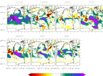
The 4×CO2 GCM-derived OLWcloud feedbacks are also
most prominent in the tropics with considerable vari-ability in the location, magnitude, and direction of peak feedback (Fig. 4). However, all models show a negative OLWcloudfeedback across the equatorial Pacific and a
pos-itive OLWcloud feedback over the Indonesia Archipelago,
Figure 4.Maps of annual-mean outgoing longwave feedback term (OLWcloudFB), as calculated using Eq. (14) and the 4×CO2results of the 7 CMIP5 models discussed in the text. Units are W m−2◦C−1.
mid-latitudes and slight negative feedbacks in the polar re-gions. These data are consistent with observations of in-creased cloud top height (Norris et al., 2016), as regions with enhanced cloudiness (increased αatm, Fig. 2) also typically
show decreased OLW (Fig. 4).
For the LGM, GCM-derived cloud feedbacks are less co-herent. Nearly all models show large changes in the tropi-cal αatm feedback, particularly across the equatorial Pacific
and Indonesian Archipelago (Fig. 3). Such changes may be suggestive of changes in the position of the intertropical con-vergence zone (ITCZ)-associated changes in deep convective cloud systems that are specific to each model (Braconnot et al., 2007; Arbuszewski et al., 2013). In addition, nearly all GCM-derived feedbacks show a reduction in αatm over the
North Atlantic (note that LGM cooling indicates that direc-tion of feedback change is opposite that shown in Fig. 3), which may be indicative of a shift in the position of the Gulf Stream seen in some models (Otto-Bliesner et al., 2006). The prominent feature in the LGM GCM-derived OLWcloud
feed-back is a large reduction in the tropics (green–blue–purple colors in Fig. 5), which is likely related to the reduction in tropical convection due to lower sea surface temperatures (Yin and Battisti, 2001). However, this spatial extent and magnitude of reduction in OLWcloud for the LGM vary
ap-preciably among the GCMs.
3.2 Radiative balance in CFE 4×CO2simulation
To compare the global radiative balance of CFE with that of the GCMs, we calculate the total change in TOA short-wave and longshort-wave fluxes per global mean surface tempera-ture change from the final 10 years of the 150-year 4×CO2
simulations (relative to the control simulation) and compare the raw GCM results with our cloud feedback-forced CFE simulations (Fig. 6). The changes in longwave fluxes in-clude the CO2forcing, which may differ by∼15 % between
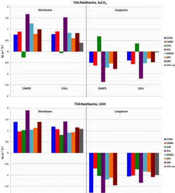
models (Andrews et al., 2012). Because the forcing is in-cluded in the longwave fluxes, the flux / temperature ratios shown in Fig. 6 are not a true “feedback”, strictly speaking; therefore, we use the term “radiative-temperature response.” However, variations in the forcings are presumably relatively small compared to variations in feedbacks. The shortwave flux / temperature ratios in Fig. 6 are true feedbacks and con-sistent with numbers reported previously (Tomassini et al., 2013).
In general, the spread of TOA shortwave and longwave radiative-temperature response in the 4×CO2CFE
Figure 5.Maps of annual-mean outgoing longwave feedback term (OLWcloudFB), as calculated using Eq. (14) and the LGM results of the 7 PMIP3 models discussed in the text. Units are W m−2◦C−1. Note that because the LGM represents a period of global cooling (Braconnot et al., 2012), the direction of change in OLWcloudis opposite that shown in these figures.
positive longwave radiative-temperature response, which is consistent with the CFE results. All other GCM and CFE simulations have positive shortwave and negative longwave radiative-temperature response that are both smaller in mag-nitude than the IPSL-based simulations.
While the relative magnitude of the CFE radiative-temperature response results captures that of the origi-nal GCM results, the absolute magnitude of the radiative-temperature response is generally slightly reduced in CFE. We also present the results from a control 4×CO2
UVic simulation, without the implementation of any cloud feedbacks (gray bar, Fig. 6). Here, the TOA short-wave radiative-temperature response is∼0.40 W m−2◦C−1 and the TOA longwave radiative-temperature response is ∼ −0.03 W m−2◦C−1, whereas the average radiative-temperature response from the GCMs are ∼0.87 and ∼ −0.55 W m−2◦C−1, respectively. Therefore, the
applica-tion ofαatmand OLWcloudfeedbacks in CFE are prominent
drivers in the spread of total TOA shortwave and longwave radiative-temperature response. In general, the GCMs show a greater reduction in global surface albedo with increas-ing temperature compared to the CFE (not shown). There-fore, the differences in surface albedo processes between the GCMs and CFE, likely explains some of the reduction in TOA shortwave radiative-temperature response magnitude in the CFE simulations.
3.3 Radiative balance in CFE LGM simulations For the CFE LGM simulations, we calculate TOA short-wave and longshort-wave radiative-temperature response at equi-librium conditions, averaged over the last 100 years of the LGM and ctlLGM experiments. Note that in this case the shortwave fluxes include forcing from prescribed ice sheets and therefore are not strictly speaking feedbacks. CFE gen-erally captures the spread of the shortwave and longwave radiative-temperature response from the GCMs although it is slightly reduced (Fig. 6). The total imbalance seems to be smaller in CFE compared with most GCMs indicating that CFE is closer to equilibrium, perhaps because it was inte-grated longer. Thus, a larger remaining imbalance could con-tribute to the larger spread in the GCMs compared with CFE. The absolute magnitude of the radiative-temperature re-sponse is mostly reduced in the CFE relative to the GCM simulations. Similar to the 4×CO2 results, the IPSL-based
Figure 6.Comparison of 4×CO2(top) and LGM (bottom) top-of-the-atmosphere feedbacks calculated from raw CMIP5/PMIP3 output from each of the seven GCMs (CMIP5/PMIP3) and from UVic simulations using GCMs-derived cloud feedbacks (UVic). Shortwave feedbacks are shown on the left, longwave feedbacks on the right. Positive values designate an increased forcing TO the climate system with increased temperature (i.e., positive feedback). Feedbacks from the UVic control simulation without cloud feedbacks is shown in gray.
3.4 Effect of CFE on modeled temperature evolution and spatial distribution
As expected, the incorporation of cloud feedbacks into CFE has a direct impact on modeled surface temperature anoma-lies in perturbed experiments. For the 4×CO2experiments,
global mean surface air temperature anomalies at the end of the 150-year simulation range from +3.9◦C (GISS) to +8.8◦C (IPSL), where the control UVic simulation with-out cloud feedbacks results in a final anomaly of +5.1◦C (Fig. 7). Only two CFE simulations (GISS and MRI) result in a year 150 temperature anomaly that is less than the UVic control, confirming that the 4×CO2net cloud feedbacks are
generally positive (see above) and consistent with the
anal-ysis of the individual models themselves (Vial et al., 2013; Tomassini et al., 2013).
The spatial variability in GCM cloud feedbacks (Figs. 2, 4) is also expressed in the 4×CO2zonal mean temperature
anomalies (Fig. 7). All models show the effects of strong po-lar amplification by the end of the 4×CO2simulations, but
Figure 7.Global mean surface air temperature anomalies for the 4×CO2(upper left) and LGM (upper right) CFE simulations. Zonal mean surface air temperature anomalies from the CFE simulations, averaged over the last 10 years of the 4×CO2simulations (lower left) and the last 100 years of the LGM simulation (lower right).
For the LGM simulations, the global mean temperature change at the end of the simulation ranges from −4.1◦C (CCSM) to −8.2◦C (CNRM), whereas the control UVic
simulation has a cooling of 5.7◦C (Fig. 7). Nearly half
of the UVic simulations show enhanced global mean cool-ing (CNRM, IPSL, and MRI) relative to the UVic control (Fig. 7), whereas the other four simulations show reduced cooling (CCSM, GISS, MIROC, and MPI). Again, zonal mean temperature anomalies at the LGM show that enhanced cloud feedbacks lead to enhanced polar amplification, but spatial differences in the magnitude of feedbacks may impact regional temperature change. For example, the CNRM-based simulation shows the strongest cooling in the southern high latitude, whereas the IPSL-based simulation has the largest cooling in the northern high latitudes (Fig. 7).
3.5 Using CFE to estimate climate sensitivity
Inter-model spread in GCM cloud feedbacks has been shown to have a large impact on the modeled sensitivity to pertur-bation in greenhouse gas radiative forcing (Fasullo and Tren-berth, 2012; Andrews et al., 2012; Sherwood et al., 2014). To estimate the effect of the cloud feedbacks in CFE on global climate, we calculate effective equilibrium climate sensitivity (1T2xC,eff)from the 150-year 4×CO2simulations
by regressing the global net downward heat flux at the TOA onto the change in temperature. The slope of this
regres-sion is the climate response parameter (α) and the inter-cept is the 4×CO2 forcing (F4xCO2)specific to each model
(Gregory et al., 2004). These values can be used to esti-mate the effective equilibrium cliesti-mate sensitivity to a dou-bling of CO2by dividing the implied global 2xCO2forcing
(F2xCO2 =F4xCO2/2) byα(Gregory et al., 2004). We
calcu-late1T2xC,efffor both the raw GCM model output as well as
the associated CFE simulations.
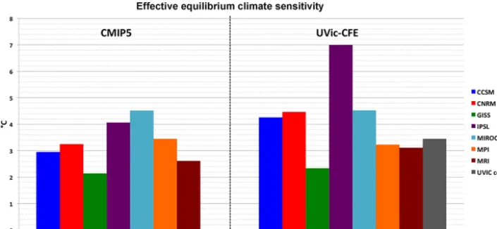
With the introduction of cloud feedbacks, CFE is able to capture much of the inter-model variability in climate sen-sitivity (Fig. 8). The seven GCMs sampled in this analy-sis show values of1T2xC,eff ranging from 2.15◦C (GISS)
to 4.10◦C (IPSL), which agrees well with Andrews et al. (2012) for those models that were used in both studies. In the CFE simulations, 1T2xC,eff values range from 2.34◦C
(GISS) to 7.00◦C (IPSL). Again, the IPSL-based CFE sim-ulation is a noticeable outlier, whereas all of the values of 1T2xC,eff in CFE are more comparable to the values from
the raw GCM output and the magnitude relative to each of the models is generally the same (Fig. 8). However, most of the CFE simulations show elevated1T2xC,effrelative to their
GCM counterpart (Fig. 8). The1T2xC,effin the 4×CO2
Figure 8.Comparison of effective equilibrium climate sensitivity (1T2xC,eff)calculated from raw CMIP5 output from each of the seven GCMs (CMIP5) and from UVic simulations using GCMs-derived cloud feedbacks (UVic). 1T2xC,eff from the UVic control simulation without cloud feedbacks is shown in gray.
GCMs. This suggests that the control UVic model’s clear-sky (without explicit clouds) feedbacks are larger than those of most GCMs. Adding the mostly positive cloud feedbacks thus makes the UVic model’s climate sensitivities consider-ably larger than those of the GCMs. Clear-sky feedbacks in the UVic model could be tuned by, e.g., varying the coef-ficients of Eq. (6) if a better match with individual GCM’s climate sensitivity was desired.
4 Discussion and Conclusions
The cloud feedbacks (αatm and OLWcloudfeedbacks)
de-rived from the GCMs and employed in CFE are gener-ally consistent between climate states (4×CO2 vs. LGM)
for each GCM, with some notable exceptions. For exam-ple, the 4xCO2αatm feedbacks (Fig. 2) are generally
consis-tent between models in showing a prominent negative feed-back across the Southern Ocean, with CCSM being the only model with a positiveαatmfeedback. However, for the LGM,
the CCSM-derivedαatm feedback is negative along with all
other models in general (Fig. 3). In addition, theαatm
feed-backs across the equatorial Pacific are not always consistent between climate states, with the CNRM-, GISS-, MIROC-, and MPI-based fields showing a pronounced difference in the direction of theαatmfeedback (Figs. 2, 3). Similarly, the
OLWcloud feedbacks across the equatorial Pacific and North
Pacific differ in magnitude and direction between the climate states in nearly all models (Figs. 4, 5). These differences likely arise due to shifts in the ITCZ and Gulf Stream be-tween climate states (Otto-Bliesner et al., 2006; Braconnot et al., 2007; Arbuszewski et al., 2013), and they suggest that such cloud feedbacks are not universal to all climate states. Furthermore, the cloud feedbacks derived from the GCMs should only be applied to a consistent climate state experi-ment when using CFE.
In general, the application of GCM-derived cloud feed-backs to CFE captures the changes in TOA radiative balance of the original GCMs, for both the 4×CO2and LGM
experi-ments. Differences in total radiative feedbacks between each GCM and the associated CFE may exist for several reasons. First, the derivation of the cloud feedbacks are parameter-ized from the original GCM results and therefore may not be a perfect representation of the full complexity of cloud radiative forcing in each GCM. This is particularly the case for the shortwave cloud feedback, which is applied using a calculation of theαatm feedback, which uses an assumption
of a global mean atmospheric transmissivity (Eq. 3). The OLWcloud feedbacks, on the other hand, are a direct
calcu-lation of the longwave cloud feedbacks from each GCM. Second, total TOA feedbacks in CFE may not perfectly match those of the source GCMs because the resulting feed-backs are still partly controlled by the control radiative bal-ance code of the UVic model. Other components of the Earth system, apart from clouds, impact the shortwave and long-wave radiative balance in UVic, which may feedback on the simulated climate in a different manner than in the GCMs. For instance, the total TOA shortwave feedbacks include the effect of surface albedo change. Therefore, differences in vegetation and sea ice dynamics and their effect on surface albedo in the GCMs relative to UVic may help explain some of the differences in the shortwave feedbacks. Similarly, the longwave feedback in UVic is in part controlled by the SAT-based parameterization of OLW in Eq. (6), which may be different from the clear-sky feedbacks in the GCMs
while capturing an important component of the Earth’s ra-diative balance that is otherwise lacking in the default UVic model. Indeed, the inclusion of cloud feedbacks leads to a large spread in surface air temperature anomalies for both the 4×CO2and LGM experiments (Fig. 7). In addition,
spa-tial variability in the cloud feedbacks (Figs. 2–5) leads to some differences in the latitudinal distribution of this temper-ature change (Fig. 7), suggesting that certain regional cloud changes may be important on the global scale. Differences in Equator–pole temperature contrast do to cloud feedbacks in CFE could impact ocean heat transport in the model.
The application of cloud feedbacks in CFE provides an important source of inter-model uncertainty that is present in CMIP5/PMIP3. Recent model–data comparisons suggest that the state-of-the-art CMIP5 simulations capture impor-tant cloud feedbacks across the observational record (Norris et al., 2016), providing assurance that the feedbacks in CFE are also within the range of observations. However, as model physics of cloud dynamics and spatial distribution continue to improve in future GCM simulations, the GCM cloud radia-tive effects can again be applied in CFE ensemble analyses to emulate the multi-model uncertainty in cloud feedbacks.
Finally, we confirm that the cloud feedbacks in each of the GCMs plays a prominent role in determining the resulting climate sensitivity of each simulation (Fasullo and Trenberth, 2012; Andrews et al., 2012; Sherwood et al., 2014). By incor-porating cloud feedbacks into CFE, we generally capture the relative spread1T2xC,effof the GCMs (Fig. 8). The absolute
magnitude of1T2xC,effis typically larger in our CFE
simula-tions relative to each of the GCMs. Since net cloud feedbacks are generally positive in CMIP5 (Vial et al., 2013; Tomassini et al., 2013), the addition of these radiative feedbacks may require a revision of the overall radiative balance in CFE. Specifically, future versions of CFE may consider the effects of cloud masking and rapid adjustment in the cloud feedback parameterization (Zelinka et al., 2013). Conversely, the full radiative balance may be adjusted through an enhanced OLW parameterization by slight modification to the constants in Eq. (6). This method of has been applied to UVic to effec-tively adjust1T2xC,eff(Schmittner et al., 2011). The CFE is
Competing interests. The authors declare that they have no conflict of interest.
Acknowledgements. This work was supported by a grant from the National Science Foundation’s Paleoclimate Perspectives on Climate Change (P2C2) program (award number 1204243). The authors thank two anonymous referees, along with the editorial staff of Geoscientific Model Development for their constructive comments and suggestions.
Edited by: K. Gierens
Reviewed by: two anonymous referees
References
Andrews, T., Gregory, J. M., Webb, M. J., and Taylor, K. E.: Forcing, feedbacks and climate sensitivity in CMIP5 coupled atmosphere-ocean climate models, Geophys. Res. Lett., 39, L09712, doi:10.1029/2012GL051607, 2012.
Arbuszewski, J., deMenocal, P. B., Cléroux, C., Bradtmiller, L., and Mix, A.: Meridional shifts of the Atlantic intertropical conver-gence zone since the Last Glacial Maximum, Nat. Geosci., 6, 959–962, doi:10.1038/NGEO1961, 2013.
Barkstrom, B. R.: The earth radiation budget experiment (ERBE), B. Am. Meteorol. Soc., 65, 1170–1185, 1984.
Barkstrom, B. R. and Smith, G. L.: The earth radiation budget ex-periment: Science and implementation, Rev. Geophys., 24, 379– 390, 1986.
Braconnot, P., Harrison, S. P., Otto-Bliesner, B., Abe-Ouchi, A., Jungclaus, J., and Petterschmitt, J.-Y.: The Paleoclimate Mod-eling Intercomparison Project contribution to CMIP5, CLIVAR Exchanges, 16, 15–19, 2011.
Braconnot, P., Harrison, S. P., Kageyama, M., Bartlein, P. J., Masson-Delmotte, V., Abe-Ouchi, A., Otto-Bliesner, B., and Zhao, Y.: Evaluation of climate models using palaeoclimatic data, Nature Climate Change, 2, 417–424, 2012.
Cess, R. D., Zhang, M., Wang, P. H., and Wielicki, B. A.: Cloud structure anomalies over the tropical Pacific during the 1997/98 El Nino, Geophys. Res. Lett., 28, 4547–4550, 2001.
Cox, P. M.: Description of the TRIFFID dynamic global vegetation model, Technical Note 24, Hadley Centre, United Kingdom Me-teorological Office, Bracknell, UK, 1–16, 2001.
Crucifix, M., Loutre, M. F., Tulkens, P., Fichefet, T., and Berger, A.: Climate evolution during the Holocene: A study with an Earth system model of intermediate complexity, Clim. Dynam., 19, 43– 60, 2002.
Driesschaert, E.: Climate change over the next millennia using LOVECLIM, a new Earth system model including the polar ice sheets, PhD thesis, 214 pp., Univ. Catholique de Louvain, Louvain-la-Neuve, Belgium, 2005.
Dufresne, J. L. and Bony, S.: An assessment of the primary sources of spread of global warming estimates from coupled atmosphere-ocean models, J. Climate, 21, 5135–5144, 2008.
Eby, M., Weaver, A. J., Alexander, K., Zickfeld, K., Abe-Ouchi, A., Cimatoribus, A. A., Crespin, E., Drijfhout, S. S., Edwards, N. R., Eliseev, A. V., Feulner, G., Fichefet, T., Forest, C. E., Goosse, H., Holden, P. B., Joos, F., Kawamiya, M., Kicklighter, D., Kienert, H., Matsumoto, K., Mokhov, I. I., Monier, E., Olsen, S. M., Ped-ersen, J. O. P., Perrette, M., Philippon-Berthier, G., Ridgwell, A., Schlosser, A., Schneider von Deimling, T., Shaffer, G., Smith, R. S., Spahni, R., Sokolov, A. P., Steinacher, M., Tachiiri, K., Tokos, K., Yoshimori, M., Zeng, N., and Zhao, F.: Historical and ide-alized climate model experiments: an intercomparison of Earth system models of intermediate complexity, Clim. Past, 9, 1111– 1140, doi:10.5194/cp-9-1111-2013, 2013.
Fasullo, J. T. and Trenberth, K. E.: The annual cycle of the energy budget. Part I: Global mean and land-ocean exchanges, J. Cli-mate, 21, 2297–2312, 2008.
Fyke, J. and Eby, M.: Comment on “Climate sensitivity estimated from temperature reconstructions of the Last Glacial Maximum”, Science, 337, 1294–1294, 2012.
Gregory, J. M., Ingram, W. J., Palmer, M. A., Jones, G. S., Stott, P. A., Thorpe, R. B., Lowe, J. A., Johns, T. C., and Williams, K. D.: A new method for diagnosing radiative forc-ing and climate sensitivity, Geophys. Res. Lett., 31, L03205, doi:10.1029/2003GL018747, 2004.
Hartmann, D. L. and Short, D. A.: On the use of earth radiation budget statistics for studies of clouds and climate, J. Atmos. Sci., 37, 1233–1250, 1980.
Hartmann, D. L., Ockert-Bell, M. E., and Michelsen, M. L.: The effect of cloud type on Earth’s energy balance: Global analysis, J. Climate, 5, 1281–1304, 1992.
IPCC Working Group I: Climate Change 2001: The Scientific Basis, Contribution of Working Group I to the Third Assessment Report of the Intergovernmental Panel on Climate Change, edited by: Houghton, J. T., Ding, Y., Griggs, D. J., Noguer, M., van der
Lin-den, P. J., Dai, X., Maskell, K., and Johnson, C. A., Cambridge University Press, 2001.
Joos, F., Prentice, I. C., Sitch, S., Meyer, R., Hooss, G., Plattner, G.-K., Gerber, S., and Hasselmann, K.: Global warming feedbacks on terrestrial carbon uptake under the IPCC emission scenarios, Global Biogeochem. Cy., 15, 891–907, 2001.
Loeb, N. G., Wielicki, B. A., Doelling, D. R., Smith, G. L., Keyes, D. F., Kato, S., Manalo-Smith, N., and Wong, T.: Toward opti-mal closure of the Earth’s top-of-atmosphere radiation budget, J. Climate, 22, 748–766, 2009.
Lu, J., Vecchi, G. A., and Reichler, T.: Expansion of the Hadley cell under global warming, Geophys. Res. Lett., 34, L06805, doi:10.1029/2006GL028443, 2007.
Marvel, K., Schmidt, G. A., Miller, R. L., and Nazarenko, L. S.: Implications for climate sensitivity from the response to individual forcings, Nature Climate Change, 6, 386–389, doi:10.1038/NCLIMATE2888, 2016.
Meissner, K. J., Weaver, A. J., Matthews, H. D., and Cox, P. M.: The role of land surface dynamics in glacial inception: a study with the UVic Earth System Model, Clim. Dynam., 21, 515–537, 2003.
Muglia, J. and Schmittner, A.: Glacial Atlantic overturning in-creased by wind stress in climate models, Geophys. Res. Lett., 42, 9862–9868, doi:10.1002/2015GL064583, 2015.
NOAA National Centers for Environmental Information, State of the Climate: Global Analysis for Annual 2015, published on-line January 2016, available at: http://www.ncdc.noaa.gov/sotc/ global/201513, last access: 6 July 2016.
Norris, J. R., Allen, R. J., Evan, A. T., Zelinka, M. D., O’Dell, C. W., and Klein, S. A.: Evidence for climate change in the satellite cloud record, Nature, 536, 72–75, 2016.
Otto-Bliesner, B. L., Brady, E. C., Clauzet, G., Tomas, R., Levis, S., and Kothavala, Z.: Last glacial maximum and Holocene climate in CCSM3, J. Climate, 19, 2526–2544, 2006.
Peltier, W. R.: Global glacial isostasy and the surface of the ice-age Earth: the ICE-5G (VM2) model and GRACE, Annu. Rev. Earth Planet. Sci., 32, 111–149, 2004.
Plattner, G.-K., Joos, F., Stocker, T. F., and Marchal, O.: Feed-back mechanisms and sensitivities of ocean carbon uptake under global warming, Tellus, 53B, 564–592, 2001.
Ramanathan, V., Cess, R. D., Harrison, E. F., Minnis, P., Barkstrom, B. R., Ahmad, E., and Hartmann, D.: Cloud-Radiative Forcing and Climate: Results from the Earth Radiation Budget Experi-ment, Science, 243, 57–63, 1989.
Schmittner, A., Urban, N. M., Shakun, J. D., Mahowald, N. M., Clark, P. U., Bartlein, P. J., Mix, A. C., and Rosell-Melé, A.: Climate sensitivity estimated from temperature reconstructions of the Last Glacial Maximum, Science, 334, 1385–1388, 2011. Sherwood, S. C., Bony, S., and Dufresne, J. L.: Spread in model
climate sensitivity traced to atmospheric convective mixing, Na-ture, 505, 37–42, 2014.
Soden, B. J. and Held, I. M.: An assessment of climate feedbacks in coupled ocean-atmosphere models, J. Climate, 19, 3354–3360, 2006.
tainties, in preparation, 2017.
Vial, J., Dufresne, J. L., and Bony, S.: On the interpretation of inter-model spread in CMIP5 climate sensitivity estimates, Clim. Dy-nam., 41, 3339–3362, 2013.