R E S E A R C H
Open Access
OpenFLUX2:
13
C-MFA modeling software package
adjusted for the comprehensive analysis of single
and parallel labeling experiments
Mikhail S Shupletsov
1,2*, Lyubov I Golubeva
1, Svetlana S Rubina
1, Dmitry A Podvyaznikov
1,3, Shintaro Iwatani
1,5and Sergey V Mashko
1,3,4*Abstract
Background:Steady-state13C-based metabolic flux analysis (13C-MFA) is the most powerful method available for the quantification of intracellular fluxes. These analyses include concertedly linked experimental and computational stages: (i) assuming the metabolic model and optimizing the experimental design; (ii) feeding the investigated organism using a chosen13C-labeled substrate (tracer); (iii) measuring the extracellular effluxes and detecting the13C-patterns of intracellular metabolites; and (iv) computing flux parameters that minimize the differences between observed and simulated measurements, followed by evaluating flux statistics. In its early stages,13C-MFA was performed on the basis of data obtained in a single labeling experiment (SLE) followed by exploiting the developed high-performance computational software. Recently, the advantages of parallel labeling experiments (PLEs), where several LEs are conducted under the conditions differing only by the tracer(s) choice, were demonstrated, particularly with regard to improving flux precision due to the synergy of complementary information. The availability of an open-source software adjusted for PLE-based13C-MFA is an important factor for PLE implementation.
Results:The open-source software OpenFLUX, initially developed for the analysis of SLEs, was extended for the computation of PLE data. Using the OpenFLUX2,in silicosimulation confirmed that flux precision is improved when13C-MFA is implemented by fitting PLE data to the common model compared with SLE-based analysis. Efficient flux resolution could be achieved in the PLE-mediated analysis when the choice of tracer was based on an experimental design computed to minimize the flux variances from different parts of the metabolic network. The analysis provided by OpenFLUX2 mainly includes (i) the optimization of the experimental design, (ii) the computation of the flux parameters from LEs data, (iii) goodness-of-fit testing of the model’s adequacy, (iv) drawing conclusions concerning the identifiability of fluxes and construction of a contribution matrix reflecting the relative contribution of the measurement variances to the flux variances, and (v) precise determination of flux confidence intervals using a fine-tunable and convergence-controlled Monte Carlo-based method.
Conclusions:The developedopen-sourceOpenFLUX2 provides a friendly software environment that facilitates beginners and existing OpenFLUX users to implement LEs for steady-state13C-MFA including experimental design, quantitative evaluation of flux parameters and statistics.
Keywords:Non-linear least-squares minimization problem, Normalized flux precision function, Partial optimization of experimental design, Convergence control of flux confidence interval bounds
* Correspondence:[email protected];[email protected]
1Ajinomoto-Genetika Research Institute, 117545 Moscow, Russian Federation 2
Computational Mathematics and Cybernetics Department, Lomonosov Moscow State University, 119991 Moscow, Russian Federation Full list of author information is available at the end of the article
© 2014 Shupletsov et al.; licensee BioMed Central Ltd. This is an Open Access article distributed under the terms of the Creative Commons Attribution License (http://creativecommons.org/licenses/by/4.0), which permits unrestricted use, distribution, and reproduction in any medium, provided the original work is properly credited. The Creative Commons Public Domain Dedication waiver (http://creativecommons.org/publicdomain/zero/1.0/) applies to the data made available in this article, unless otherwise stated.
Background
Metabolic flux analysis (MFA) plays a key role in systems biology because intracellular fluxes, i.e., in vivo reaction rates through different pathways within an intact living cell [1], are the functional output of all conventional gen-etic and metabolic regulatory systems and determine the physiological phenotype of the cell [2].
In recent decades, a metabolic steady-state version of
13
C-labeling-based MFA (13C-MFA) has become the best developed and most powerful method for quantifying intracellular fluxes when all fluxes and metabolite concen-trations can be considered to be (at least approximately) constant [2-4]. 13C-MFA, applied to microbial, plant and mammalian systems, has been increasingly used in sys-tems biology and metabolic engineering [5-7], biotechnol-ogy and medicine [8-10].
Due to the high complexity of native metabolic net-works,13C-MFA typically involves the use of a simplified stoichiometric model in which only the key pathway re-actions of the central carbon metabolism and the set of lumped targeted biosynthetic reactions are parameter-ized before the assumed model-based fluxes are inferred from measurable quantities [11].
Concerning the experimental data applied in13C-MFA, the physiological/extracellular fluxes or effluxes (e.g., biomass precursor drain, substrate uptake, and product excretion rates) and13C-labeling patterns (i.e., isotopomer distributions) of metabolic products resulting from feeding partially 13C-labeled substrates (tracers) are used. These effluxes are determined from the time courses of cellular dry weight and extracellular metabolite concentrations during cultivation [12]. The 13C-isotopomers generated due to the metabolic conversion of tracers are detected through nuclear magnetic resonance (NMR) spectroscopy [13], mass spectrometry (MS) [14], and/or tandem MS (MS/MS) [15].
Prof. W. Wiechert and co-workers significantly contrib-uted towards formalizing the framework for 13C-MFA: from measured effluxes and intracellular labeling informa-tion the intracellular fluxes could be computed [16-19]. On this basis, several mathematical models have been developed that can simulate a unique profile of isotopo-mer abundance for the fluxes with assigned parameters by describing the propagation of labeled atoms from the tracer through an assumed metabolic network according to the known atom rearrangements for each reaction [18,20-26]. All simulations are providing under the essential assumption that the possible isotopic mass effects [27] are negligible, i.e., that the labeling states of the metabolites do not influence the rate of their enzymatic conversion [16]. The goal of 13C-MFA is to determine the set of initially unknown flux parameters that mini-mizes the differences between experimentally observed and simulated measurements. In mathematical essence,
this set is a solution of a large-scale non-linear parameter estimation problem [28]. Analytical solutions of this prob-lem are available only for the simplest systems. Therefore, the values of the assumed fluxes must generally be in-ferred from the experimental datasets through computer model-based interpretation using an iterative least-squares fitting procedure [2,3,26].
Several high-performance computational software suites for performing flux calculations have been developed and described, e.g., 13CFLUX [29] and its reinforced version– 13CFLUX2 [30], METRAN [31,32], OpenFLUX [33], FIA [25], influx_s [34], OpenMebius [35].
These software toolboxes most often automatically gen-erate metabolite and isotopomer balance models relying on an initially user-defined simple notation of metabolic networks and the known atom transitions occurring in biochemical reactions. Then, starting from the generated models and from measured effluxes that must be con-strained within the obtained error ranges, semi-random guesses regarding intracellular fluxes are used to simulate
in silico 13C-labeling patterns of targeted metabolites, which, in turn, are compared with the measured patterns. This process is repeated until a satisfactory match to the measurable quantities is achieved, i.e., the constrained non-linear least-squares minimization problem (NLLSP) is solved [29]. According to the rules of regression ana-lysis, providing a statistical goodness-of-fit test of the adequacy of the applied flux model is required, at a minimum, after determining the optimized fluxes [28,36]. Then, linearized statistics [17,37,38], a non-linear-based search algorithm [28], and/or the Monte Carlo approach [39,40] are used to estimate the precise flux resolution, i.e., the uncertainty of the determined fluxes. The opti-mized parameters of the fluxes and their confidence intervals in the statistically adequate user-made metabolic model must be obtained as the concerted results of these computations.
When the13C-labeling data were obtained from NMR in the early stages of13C-MFA development, each analysis was typically performed on a single labeling experiment (SLE), primarily for cost reasons [41]. Implementing highly sensitive MS- [42-44] and MS/MS-mediated [15,45] measurements, which are development approaches that involve 13C-tracer experiments at a miniaturized scale [46,47], led to a significantly increased accessibility and decreased cost of labeling experiments (LEs). Thus, it has become possible to realize the advantages of parallel labeling experiments (PLEs), in which two or more LEs are initiated from the same seed culture and conducted in parallel under the same experimental conditions dif-fering only in the set of13C-tracers applied [48-53].
of the same compound or multiple labeled substrates [32,54-57]. Studies have shown that achieving optimal resolution of fluxes from different parts of the central carbon metabolism requires different13C-tracers [19,48,58]. Several sophisticated experimental design strategies have been adopted to improve the desired flux precision [19,32,36,49,54,56,59-64]. Therefore, the use of only one set of tracers will likely not maximize the resolution of all fluxes in SLEs, particularly when a large-scale metabolic model is employed [28,65].
According to previous studies [53,58,66,67], there are several advantages of using PLEs for13C-MFA compared with an SLE-based approach. In general, the data from each LE are integrated to achieve an improved flux reso-lution, primarily due to the synergy of the complemen-tary information used for fitting to the single metabolic model [48,53,58,66]. Indeed, the latest applications of the COMPLETE (short for COMplementary Parallel Labeling Experiments TEchnique [58]) MFA approach employing all six singly labeled glucose tracers to evaluate metabolic fluxes resulted in the most accurate and precise flux pa-rameters obtained thus far for wild-typeE. colias well as for some metabolically engineered strains of the bacterium [58,67]. However, for laboratories lacking in-house experi-ence, one crucial factor in the implementation of the PLE approach is the availability of a free, ready-to-use software package allowing the successful manipulation of the complex data obtained in PLEs, which is necessary for comprehensive flux analysis.
In the present study, the open-source software Open-FLUX [33], which uses an elementary metabolic unit (EMU) decomposition-based algorithm to generate an isotopomer balance model [26] and was initially devel-oped for SLE analysis, has been extended for the computation of PLE data (see, Additional file 1:SF-1.3. The methodology of PLE data implementation is rather clear, and one of the possible algorithms has been earlier schematically described in [53]. The expertized investi-gators have already adjusted their home-made13C-MFA software by PLEs-mediated data (see, [66] for review). Currently, additional MATLAB-based scripts have been appeared on the OpenFLUX homepage (http://openflux. sourceforge.net) that demonstrated to users how the data of two labeling experiments conducting in parallel could be implemented in the already existing software. The presentedopen-sourceOpenFLUX2 provides a friendly soft-ware environment that facilitates beginners and existing OpenFLUX users to manipulate with SLE- and PLE-based data, for experimental design, determination of flux pa-rameters, and for broaden evaluation of flux statistics.
Using OpenFLUX2, directin silicosimulation confirmed that the flux resolution was improved when13C-MFA was provided with PLE data that were fitted to and integrated with the common metabolic model as compared with the
individual analysis of each LE. Additionally, the best flux resolution was achieved in the analysis of PLE results when the choice of tracer for each provided LE was based on a computed experimental design targeted to minimize the approximated variances of several fluxes from the different parts of the assumed metabolic network. The statistical methods of analysis of the obtained experi-mental and simulated data, followed by a goodness-of-fit test of the adequacy of the applied metabolic model, have been extended in OpenFLUX2, including the statis-tical conclusions concerning the feasibility of the obtained flux parameters in the final report and the flux confidence intervals estimated at the desired significance level. In turn, the flux confidence intervals could be computed in OpenFLUX(2) using different methods, but up today the most dependable and precise approach is a fine-tunable Monte Carlo-based determination of the flux variances, which are dependent on the randomly corrupted measured data [33,39] and that has been modified in OpenFLUX2 due to implementation of a convergence control and visualization of computation results.
Following the original position of the OpenFLUX au-thors [33], OpenFLUX2, which is an extended version of the already available software, has been developed as
open-source software. We hope that OpenFLUX2 will be useful to research groups applying13C-MFA, particularly for beginners not yet experienced in fluxomics analyses. Additionally, the availability of the OpenFLUX2codecould promote further improvement of the software based on the experiences of different researchers. OpenFLUX2 can be downloaded from SourceForge (http://sourceforge.net/ projects/openflux2).
Results
Key features of OpenFLUX2 software
OpenFLUX2 was developed as an extension of the OpenFLUX software. New calculation facilities were added, mostly as extensions of the initial options, with-out dramatic changes in the parent content. Moreover, the initial forms of the model and experimental data setup, together with results representation, were main-tained as much as possible during the development of OpenFLUX2 to facilitate the transition from one ver-sion to the other. In the present study, the procedures that were developed previously in OpenFLUX and retained in OpenFLUX2 without essential modifications are in-dicated as “OpenFLUX(2)”, and only the added/modi-fied elements are indicated as being implemented in OpenFLUX2.
To clarify the essence of the modifications implemented at the stage of OpenFLUX2 software development, the following items are schematically described in Additional file 1: (SF-1.1.) the assignment of free fluxes, followed by (SF-1.2.) flux variability analysis; (SF-1.3.) the calculation
Shupletsovet al. Microbial Cell Factories2014,13:152 Page 3 of 25
of optimized fluxes through iterative fitting; (SF-1.4.) a goodness-of-fit analysis of the adequacy of the metabolic model; (SF-1.5.) local linearized statistical approximations; and non-linear-search of the optimal flux confidence in-tervals (SF-1.6.), where, in particular, the introducing a convenient concept,“the normalized flux precision” func-tion, is described, as well; (SF-1.7.) – a fine tunable and convergence-controlled Monte Carlo-based approaches for precise determination of the optimized flux confidence intervals according to“discarding” strategy at the pre-determined confidence level, significantly modified at the stage of implementation in OpenFLUX2. The main aim of this description is to demonstrate that the indi-vidual procedures are essential interconnected parts of a unique solution to a complex optimization problem, where the statistical significance of the calculated model-based parameters must be verified via the comprehensive goodness-of-fit of the model’s adequacy. As an auxiliary
aim of this part, it is a rather short, but slightly (in com-parison with the excellent review [4]) mathematically-enriched introduction in the13C-MFA background that could be helpful, especially for beginners, to repair their knowledge by essential parts of linear algebra and statistics.
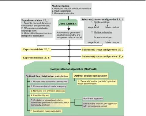
The workflow of OpenFLUX software consists of two components: (i) the automated set-up of stoichiometric and isotopomer balance models from user-supplied data, performed by Java PARSER, and (ii) the application of the generated models to the 13C-MFA of SLEs for flux parameter estimation and sensitivity analysis, performed by a set of specially developed MATLAB functions. The modifications introduced in OpenFLUX2 can be divided into two types (Figure 1). First, a set of new options related to statistical analysis of the flux evaluated from SLE data and experimental design facilities were added. Second, the new software was extended to perform
metabolic flux analysis of PLE-based data. Here, the PLE concept is considered as determined in [66]; PLE-based design means that several tracer experiments that are started from the same seed culture to minimize biological variability, and must be performed independently under identical conditions on the same substrate(s), using differ-ent tracer(s).
Because an13C-MFA PLE-based approach requires the simultaneous fitting of several datasets obtained from independent LEs to a single model, there is no major difference in the spread-sheet model set up and the consequent automated generation of stoichiometric and isotopomer balance models by the Java PARSER for PLEs and SLEs in OpenFLUX2. The set of substrates is fixed during the model generation step, and individual substrate tracer configurations are then defined by the user for each LE constituting the PLE together with the corresponding measured data (Figure 1). The option to use either a single label or a labeling mixture for each sub-strate in the PLE is provided by OpenFLUX2, as was pre-viously provided in OpenFLUX for SLEs. Thus, all of the introduced modifications were finally concentrated in the MATLAB-based portion of the computational algorithm.
Comprehensive flux analysis of aCorynebacterium glutamicummodel, as an example, using OpenFLUX2 software
The C. glutamicum model
The specific features of the developed OpenFLUX2 software were illustrated via thein silicosimulation of a set of SLEs and PLEs followed by their comprehensive
13
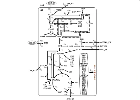
C-MFA. The Corynebacterium glutamicum metabolic model initially proposed for anL-lysine-overproducingC. glutamicumstrain by Becker et al. [68] and later used to demonstrate the possible applications of OpenFLUX software [33] was chosen (with minor changes; see Methods) as the object of the computational simulation and 13C-MFA. This model, schematically presented in Figure 2, accounted for the main central metabolic pathway, the biosynthetic pathways for several excreted products, including lysine as the main product, and anabolic demand. CO2-mediated carbon transfer was
accounted for using expression reactions, accompanied by CO2production/consumption, in an explicit manner.
The bi-directional reactions were represented as non-negative forward and reverse fluxes. Finally, the metabolic model was composed of 51 unknown fluxes balancing 36 metabolites, resulting in the stoichiometric matrix S, dim(S) = (36 × 51), with a residual 15 degrees of freedom. The degrees of freedom were associated with the follow-ing free fluxes: experimentally determined effluxes, in-cluding biomass biosynthesis (1 flux), effluxes of secreted products (5 fluxes), and the glucose uptake rate (1 flux); reverse branches of five bi-directional reactions; and
free irreversible reactions associated with branch points. An isotopomer model was generated automatically under the assumption that the mass isotopomer distribu-tions of the following metabolites were measured: alanine, valine, threonine, aspartate, glutamate, serine, phenylalan-ine, glycphenylalan-ine, tyrosphenylalan-ine, and trehalose. Application of the EMU approach offered by OpenFLUX(2) led to a major simplification of the isotopomer model (see Methods).
Circumstantiation of flux parameters for the computer simulations
The full set of fluxes necessary for the simulation of in silicoSLEs and PLEs for the defined model was unfortu-nately not directly available from previously published materials [33,68]. Thus, the evaluation of fluxes from published experimental data was repeated in the present study. To this end, a new constrained NLLSP was designed based on a modified metabolic model, with assigned free fluxes, previously measured [68] effluxes with their variances, and MIDs with variances assumed to be 0.15 mol% (see Methods). Solutions of the designed NLLSP were obtained by OpenFLUX2 using a gradient-based local optimization method with the assistance of MATLAB’s FMINCON function (see Additional file 1:
SF-1.3., for details). To determine the global mini-mum, 100 independent iterative trials were performed with an arbitrary set of initial free fluxes, θk∈ℜp,k=
1, 2,…, 100, where ℜp indicates a feasible constrained domain in the free flux variation space (see Additional file 1: SF-1.2.). These trials resulted in a set of flux esti-mates, uð⌢θkÞ;k¼1;2;…;100 , corresponding to the minimum values of the objective functionSSRSLEf k in Eq. (S−1.3.7), which were reached in each k-th trial. According to the optimization report, all of the provided trials were terminated successfully due to the achievement of the given termination tolerance (ΤΤ= 1 × 10⁻⁴) within the constraint violation tolerance. Theχ2-based goodness-of-fit confirmed the model adequacy (see Additional file 1:
SF-1.4., for details) for 82 (at a significance level of α= 0.05) and 34 (atα= 0.32) of the 100 obtained values ofΞk¼2⋅ SSRSLE
f
kas follows:
χ2
α=2ðW−pÞ<Ξk<χ21−α=2ðW−pÞ ð1Þ
where W is the number of independent measurements, andpis the number of estimated free fluxes ((W−p= 21) in this case). All essential information concerning the obtained solutions is presented in Table 1 (Exp_1.1), Additional file 2: Figure SF-2.1, and Additional file 3: Table SF-3.3. A minimal value of the Ξ function was registered for the group of 26 trials, and all fluxes from these solutions corresponded practically to the same
Shupletsovet al. Microbial Cell Factories2014,13:152 Page 5 of 25
point, uð⌢θÞ∈ℜn, in the feasiblen-dimensional space for the flux variation.
The flux identifiability analysis, which was based on
model linearization and on the computation of
Null Jfð⌢θÞ
in Eq. (S−1.5.9) (see Additional file 1:SF-1.5.),
was provided for the obtained statistically available solu-tion as described by Yang et al. [69]. This analysis resulted in the conclusion that only a unique set of flux parameters for the global minimum of the constrained NLLSP could be computed numerically; because the calcu-lated null space matrix was empty. The
goodness-of-fit analysis was finalized by confirming theΝ(0, 1) dis-tribution of the individual variance-weighted residuals inΞð⌢θÞ(see Additional file 1:SF-1.4.for details).
The obtained statistically acceptable solution of the con-strained NLLSP, uðθ⌢Þ, primarily coincided with the previ-ously published [33,68] values of fluxes in the range of the earlier evaluated flux confidence intervals (Additional file 2: Figure SF-2.2). Thus, all flux parameters, including pre-viously unavailable, were evaluated and assigned as the true values for the assumed metabolic model,u(θtrue).
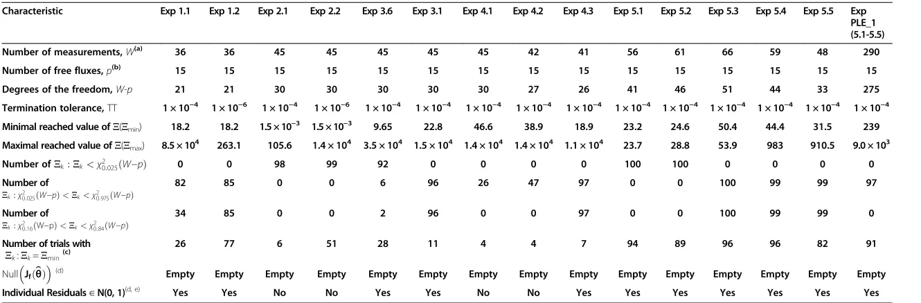
Table 1 General characteristics of the obtained NLLSP solutions
Characteristic Exp 1.1 Exp 1.2 Exp 2.1 Exp 2.2 Exp 3.6 Exp 3.1 Exp 4.1 Exp 4.2 Exp 4.3 Exp 5.1 Exp 5.2 Exp 5.3 Exp 5.4 Exp 5.5 Exp PLE_1 (5.1-5.5)
Number of measurements,W(a) 36 36 45 45 45 45 45 42 41 56 61 66 59 48 290
Number of free fluxes,p(b) 15 15 15 15 15 15 15 15 15 15 15 15 15 15 15
Degrees of the freedom,W-p 21 21 30 30 30 30 30 27 26 41 46 51 44 33 275
Termination tolerance,TT 1 × 10⁻⁴ 1 × 10⁻⁶ 1 × 10⁻⁴ 1 × 10⁻⁶ 1 × 10⁻⁴ 1 × 10⁻⁴ 1 × 10⁻⁴ 1 × 10⁻⁴ 1 × 10⁻⁴ 1 × 10⁻⁴ 1 × 10⁻⁴ 1 × 10⁻⁴ 1 × 10⁻⁴ 1 × 10⁻⁴ 1 × 10⁻⁴
Minimal reached value ofΞ(Ξmin) 18.2 18.2 1.5 × 10⁻³ 1.5 × 10⁻³ 9.65 22.8 46.6 38.9 18.9 23.2 24.6 50.4 44.4 31.5 239
Maximal reached value ofΞ(Ξmax) 8.5 × 10⁴ 263.1 105.6 1.4 × 10⁴ 3.5 × 10⁴ 1.5 × 10⁴ 1.4 × 10⁴ 1.4 × 10⁴ 1.1 × 10⁴ 23.7 28.8 53.9 983 910.5 9.0 × 10³
Number ofΞk:Ξk<χ20:025ðW−pÞ 0 0 98 99 92 0 0 0 0 100 100 0 0 0 0
Number of Ξk:χ2
0:025ðW−pÞ<Ξk<χ20:975ðW−pÞ
82 85 0 0 6 96 26 47 97 0 0 100 99 99 97
Number of Ξk:χ2
0:16ðW−pÞ<Ξk<χ20:84ðW−pÞ
34 85 0 0 2 96 0 0 97 0 0 100 99 99 0
Number of trials with Ξk:Ξk=Ξmin(c)
26 77 6 51 28 11 4 4 7 94 89 96 96 82 91
Null Jfð⌢θÞ
(d) Empty Empty Empty Empty Empty Empty Empty Empty Empty Empty Empty Empty Empty Empty Empty
Individual Residuals∈N(0, 1)(d, e) Yes Yes No No Yes Yes No No Yes Yes Yes Yes Yes Yes Yes
To determine the global minimum of the NLLSP, 100 independent iterative trials were provided with an arbitrary set of initial free fluxes for all representedin silicoLEs. All iterative trials were terminated successfully for each independent NLLSP. More detailed characteristics for all performedin silicoexperiments are listed in Additional file3.
(a)
In the case of the SLE, the vector of the measured data consists of both measured MID values and measured effluxes. In the case of the PLE, the vector of the measured data consists of the measured MIDs and effluxes that were available for each SLE.
(b)
The measured effluxes are included in the set of free fluxes, constrained according to Eq. (S−1.2.2) with experimentally determined parametersqmea eff ;σmeaeff . (c)
The values ofΞkthat were obtained during different iterative trials were assumed to be equal to theΞminif the values were different from theΞminby a value less than or equal to the TT level, i.e.,Ξk−Ξmin≤TT. (d)
The analysis was performed for the NLLSP solution, which provided the minimal achieved value ofΞ, i.e.,Ξmin. (e)
The individual variance-weighted residuals were recognized to be not distributed as N(0, 1) if both the Kolmogorov-Smirnov test, provided by MATLAB, rejected this hypothesis and the individual residual plot revealed unpredictable high values for the individual residual/group of the individual residuals or, in contrast, unpredictable small values for the primary part of the individual residuals.
Shupletsov
et
al.
Microbial
Cell
Factories
2014,
13
:152
Page
7
o
f
2
5
http://ww
w.microbialce
llfactories.c
om/content
u(θ)∈ℜnand primarily differed fromu(θtrue) in the values
of two fluxes: θ22: PYR + CO2→F OAA and (vdep)23:
OAA→FPYR + CO2 (Figure 3(A)). The value of the re-sidual net flux for these reactions, vnet= |θ22−(vdep)23|,
remained practically constant for all χ2-statistically ac-ceptable trials. The possible existence of local minima of theΞ(θ) function with a parameter ofθ22, as an alternative
to its true values, was tested. As shown in Additional file 2: Figure SF-2.3, the minimized sum of the squared residuals as a function ofθ22represents one distinct
glo-bal minimum in the neighborhood of (θ22)true followed
by a gentle decreasing slope, which ends nearly as a plateau.
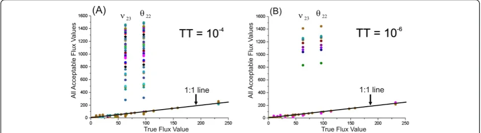
Thus, additional solutions of the constrained NLLSP may be obtained in independent trials starting from the random initial values of the free fluxes, resulting in the premature termination of the computer search for the global minimum due to the discovery of a termination tolerance (TT). Indeed, repeated numerical solutions of the same constrained NLLSP under conditions with a decreasing TT of the objective function value sloped from the default value of 1 × 10⁻⁴up to the more precise value ofΤΤ= 1 × 10⁻⁶(see Additional file 1:SF-1.3., for details), resulting in an increased number of trials that reached the global minimum (77 of 100, in contrast to 26 in the previous calculations; see Table 1 (Exp_1.1;
Exp_1.2) and Additional file 2: Figure SF-2.1), with a decreasing number of alternative statistically accept-able solutions (Figure 3(B)).
Thus, a unique optimal set of fluxes for the statistically adequate metabolic model was obtained: uðθ⌢Þ≡uðθtrueÞ. Then, new GC-MS-based “experimental data,” i.e., new MIDs, could be generated through directin silico simu-lation describing the propagation of13C atoms from dif-ferent tracers through a metabolic network with known flux parameters (see Methods).
13
C-MFA for in silico SLEs with [1-13C]-glucose as a tracer Initially, the simulation was provided for 99% of [1-13 C]-glucose as a tracer. The new set of MIDs was generated as described in Methods, excluding the last step of data corruption. To confirm that flux estimations could be un-ambiguously inferred from the obtained non-noised data, these simulations were used as the experimental data, with assumed MID variances equal to 0.4 mol%, and the as-signment of all effluxes as variable free fluxes constrained in the range of the 95% confidence intervals with the standard deviations determined in [68] (see Additional file 3:Table SF-3.3). The solution to the corresponding constrained NLLSP was obtained using OpenFLUX2 software according to the standard procedure described above with details presented in Table 1 (Exp_2.1). In total, 98 values of Ξi, which corresponded to solutions
from the total obtained set of uð⌢θiÞ;i¼1;2;…;100 , were smaller than the upper, and even the lower, critical threshold values,χ2
0:975ðW−pÞandχ20:025ðW−pÞ, respect-ively, at the 95% confidence level and with (W−p) = (38 + 7)−(8 + 7) = 30 degrees of freedom. Moreover, the group of trials (6 solutions atΤΤ= 1 × 10⁻⁴and 51 solu-tions in the case of TT decreased to 1 × 10⁻⁶; see Table 1
(Exp_2.1; Exp_2.2)) had a minimal value of 1.5⋅10−3, which was significantly less than the minimal threshold. Such a questionably small value for the objective function generally indicates possible overfitting of the applied model. However, in our case, the cause stems from the so-lution of the inverse task without corrupting the “experi-mental” data generated at the stage of direct simulation. The same cause resulted in the negative evaluation of the individual weighted residuals inΞi according to the
nor-mality test, and the null hypothesis (concerning Ν(0, 1) distribution of residuals) was rejected. The flux estimates that corresponded to the solutions of the group with the minimal Ξi that was reached were assigned as reference
fluxes, i.e.,u(θref). Confirmation of flux identifiability was obtained based on the empty null space for the Jacobian matrix calculated at pointθ=θref. As shown in Additional file 3: Table SF-3.5, the obtained reference flux values are extremely close to the true values used for data generation.
The next stage of the simulation was the generation of “experimental data” that were closed to results that could be obtained in real experiments. The values of the previ-ously simulated MIDs and the measured effluxes were corrupted with the Ν(0,σmea) normally distributed ran-dom errors using the Statistics Toolbox of MATLAB. Five (L= 5) obtained sets of data,xmea
i ¼ xi1;xi2;…;xiw
Τ;
i¼1; 2;…;Lwere used for calculation of mean, and unbiased es-timator of the variance, respectively:
μmea j ¼ 1 L⋅ XL i¼1
xij; σmeaj ¼
ffiffiffiffiffiffiffiffiffiffiffiffiffiffiffiffiffiffiffiffiffiffiffiffiffiffiffiffiffiffiffiffiffiffiffiffiffiffiffiffiffiffiffiffiffi
1
L−1
ð Þ⋅
XL
i¼1
xij−μmeaj
2
v u u t
ð2Þ
for each fromwMIDMIDs andweffeffluxes, (w=wMID+
weff), and to assign theSSRSLEf objective function that
fi-nally determines the constrained NLLSP (S−1.3.8).
Sta-tistically acceptable solution (corresponding to the value 9.65 ofΞ(θ) function (for the group of 27 from 100 per-formed trials) that was smaller even the lower threshold,
χ2
0:025ð Þ ¼30 16:79
) at the 95% confidence level, with
Ν(0, 1) distributed weighted residuals, was found using
OpenFLUX2 (Table1(Exp_3.6)).
Monte Carlo-based and non-linear approaches for determination of flux confidence intervals
At the final stage of the13C-MFA performed for the con-sidered above constrained NLLSP, accurate 68% and 95% confidence intervals (CIMC
0:68 andCIMC0:95, respectively) were computed for the optimized fluxes initially by fine-tunable and convergence-controlled Monte Carlo-based approach implemented in OpenFLUX2 for this purpose (see Additional file 1: SF-1.7. for details). According to [39], Monte Carlo-mediated analysis of flux statistics was carried out on the basis of a discrete approximation of optimized flux estimation distributions obtained in L multi-trials when the experimental data for each trial, comprising mea-sured MIDs and effluxes, were artificially generated by corrupting of real initial data with normally distributed random errors. So, consecutive providing ofLoptimization trials finally resulted inL-set of optimized flux estimations:
U ⌢QL ¼ uð ⌢ θ1Þ; uð
⌢
θ2Þ;…; uð ⌢
θjÞ;…; uð ⌢ θLÞ
;
ð3Þ
where⌢QL¼
ð
⌢θ1;θ⌢2;…;⌢θLÞ
anduð
θ⌢jÞ
¼ð
u1ðθ⌢jÞ;u2ð⌢θjÞ;…;unð⌢θjÞ
Þ
Τ;j¼1;2;…;L. Finally, the upper and lower
bounds of the CIMCγ confidence interval at a determined
confidence level ofγ were evaluated for each flux on the
basis of these distributions according to “discarding” or
“mean-varianced” strategies (see Additional file1:SF-1.7.,
for details, and Figure 4 for clarity). In OpenFLUX2, the
first group of the tunable parameters was implemented in the Monte Carlo-based procedure which modifications could increase/decrease the precision of global minimum search during optimization process in each trial. It was ne-cessary to tune these control parameters up to the levels when their further modification does not significantly de-crease the width of CIMCγ ð Þui . Testing the several control parameters of the first group resulted in a set of their de-fault values provided the convergence of the CIMCγ ð Þui bounds. Evaluations of these parameters, partially, were presented in the Additional file 2: Figure SF-2.4 as direct visualization of the computed interval bounds in depend-ence on provided trials at the different values of control parameters.
Usually, the Monte Carlo search of CIMC
γ ð Þui bounds is based on an assumption that their estimated values have to converge in case of significant increasing of the total number of trials. So, the number of trials, L, is one of the most important parameters of Monte Carlo-based procedure, and it has to be optimally chosen (L=LMAX) forCIMCγ ð Þui precise determination in a reasonable com-putation time. The special procedure was implemented in OpenFLUX2 for a control of an essential number of optimization trials that was performed during target flux
CIMCγ ð Þui bound estimation. This control finalizing in determination of all CIMC
γ ð Þui , could be realized ON-LINE, with a help of specially preset control parameters (the second group of parameters implemented for fine tuning of the Monte Carlo-based search procedure), or according to direct user’s decision based on visualization of estimated bound plots in dependence on the currentL, and flux estimation histograms that could be presented after the predeterminedLMAXtrials were performed.
The developed Monte Carlo-based approach was used for determination of CIMCγ ð Þui for the solution of the constrained NLLSP described above (Table 1 (Exp_3.6)). The optimized flux parameter distributions were ob-tained forLMAX= 500 trials using the default set of tun-able control parameters that facilitate search of global minimum in each trial of the applied “multi runs per trial”fitting strategy (NAS=3, KNR=50, ΤΤ¼110−4; ε¼110−4, see Additional file 1: SF-1.7.,for details). Then, for all 51 fluxes of assumed metabolic network the sliding control was performed for upper and lower bounds of CIMCγ ð Þui evaluated initially according to “discarding” strategy (i.e., bounds of
CI
MCγ −1ð Þ
u
i , seedefinition in Additional file 1: SF-1.7.) with the “ win-dow” size equaled to 40 trials. As could be seen from
Shupletsovet al. Microbial Cell Factories2014,13:152 Page 9 of 25
Additional file 3: Table SF-3.6, and Figure 5 (the later presented the convergence process of confidence bounds of the CIMC0:95−1ðθ22Þ interval, as example), the δMCðL=U−1ÞB (defined by Eq. (S−1.7.7)) relative spreadings for the both upper and lower bounds of CIMC−1
0:95 ð Þui for 42 from 51 fluxes were dispersed between 0.1 and 1.0% in
the last “window”, that could be considered as rather rigorous conditions of convergence. Moreover, if a
value of δðMCL=U−Þ1B γ;i;Q⌢L;M
had been equaled to 1.0%
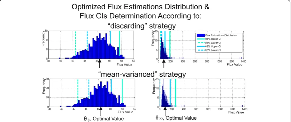
as the predetermined threshold, this level of conver-gence was achieved for more than 70% fluxes after already 20 – 50 optimization trials performed. The Figure 4Determination of flux confidence intervals at a confidence level ofγusing the Monte Carlo approach based on multiple parameter estimations.For each ofLMAX= 500 trials (simulations), all MIDs and measured efflux values were corrupted by random noise with a given standard deviations, and fluxes were estimated via least-squares optimization. Then, the estimations of each flux obtained inLMAXtrials were sorted in ascending order followed by performing of“discarding”or“mean-varianced”strategies for determination of flux confidence intervals at the confidence level ofγ,CIMC−1
γ orCIMCγ −2, respectively, (see Additional file 1:SF-1.7.). The computation of the 68% and 95% confidence interval
bounds for the⌢θ8and⌢θ22fluxes provided by both Monte Carlo-based strategies are presented as examples of estimates that are distributed rather
symmetrically or non-symmetrically, respectively, around the optimized values of fluxes (indicated by the cursor).
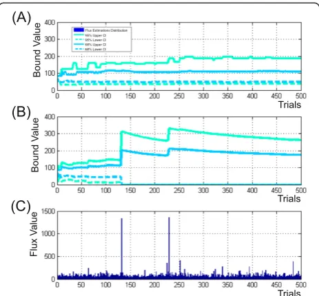
Figure 5Visualization of theθ22flux confidence interval bounds convergence.Achieved as could be seen in the“window”due to an
residual 30% of determined bounds converged after 400–420 trials according to these rigorous conditions. Eight residual fluxes (θ10;θ12;v13;θ14;θ22;v23;v29andv36) demonstrated the convergence at the relax conditions for upper and/or lower bounds, when δMCðL=U−1ÞB≤10% at the level of confidenceγ= 0.95, and this criterion was satisfied when 200 – 440 trials were performed. Five fluxes (θ10;θ14;θ31;v29andv36) had the specific feature: the values of lower bounds of their CIMC0:95−1ð Þui were closed to zero. So, these bounds, manifesting the obvi-ous convergence, had to be restricted at the level of ab-solute (not relative) value of spreading (defined in Eq. (S−1.7.6)), e.g.,ΔMCLB−1ð Þγ ≤2. In any case, all bounds of
CIMC−1
γ ð Þui could be obviously determined after the Monte Carlo-based optimized flux estimation had been obtained after LMAX =500 performed trials in case of “discarding”strategy was used. In case of“mean-varianced” strategy was applied, the main part ofCIMC0:95−2ð Þui (see def-inition in Additional file 1: SF-1.7.) bounds (for 41 of 51 fluxes) converged earlier than LMAX trials were per-formed under the rigorous convergence conditions, bounds for six additional fluxes demonstrated the convergence under relaxed conditions, and the corresponding bounds ofCIMC0:95−2ð Þui were rather closed to the earlier determined boundsCIMC0:95−1ð Þui . At the same time, the upper bounds for four residual fluxes (v9;θ10;θ22; and v23) did not finalize the convergence process after 500 performed trials (Figure 6B): their minimal upper bound values of
CIMC0:95−2ð Þui were gradually decreased in dependence on increasedLat the late stage of computation, nevertheless, they remained significantly higher than the corresponding upper bounds of CIMC0:95−1ð Þui (Figure 6A). As could be seen from the (Figure 6C), the reason of this rather slow-speed convergence of several flux bounds was appearance of a small quantity of flux estimations significantly exceeded the ordinary values: “mean-varianced” strategy could not discard these outstanding values and had to accumulate a lot of usual estimations for significant decreasing the to-tally calculated“mean”.
Summing up, it could be concluded that obtaining a proper approximation of the optimized flux parameters was the most important part of the Monte Carlo based search of CIMCγ ð Þui : even rather small quantity of signifi-cantly differed“outstanding”values in the flux estimations distribution that were obtained when the global minimum was not achieved in the fitting procedure, could signifi-cantly increase the width of the evaluatedCIMC
γ ð Þui . In the tested cases, the convergence of CIMC
γ ð Þui bounds was achieved faster (at the smaller number of the performed trials) if the“discarding”, but not“mean-varianced”strategy of the bound determination was used. So, the“discarding” strategy manifested significantly higher resistance for these
occasional“outstanding”estimations. Moreover, this strat-egy was preferable to demonstrate the asymmetric charac-ter of optimized flux estimation distribution resulting in the asymmetric locations of the upper and lower bounds presented simultaneously forCIMC−1
0:95 ð Þui, andCIMC0:68−1ð Þui , in comparison with symmetric locations of their bounds obtained in case of“mean-varianced”strategy was used (Figure 4).
The later feature of theCIMC−1
γ ð Þui bounds corresponded well with the parameters of CIn−lin
γ ð Þui independently ob-tained by non-linear search developed by Antoniewicz et al. in [28] and implemented in OpenFLUX (see Additional file 1:SF-1.6.for details). All obtained data were presented in the Additional file 3: Table SF-3.6. As could be seen, the most part of CInγ−linð Þui parameters coincided rather well with Monte Carlo-based results, especially withCIMC−1
γ ð Þui bounds (this was true from 39 of 51 fluxes). Nevertheless, in several cases evaluations of theCIγ(ui) bounds given by Monte Carlo and non-linear approaches differed, and some times significantly (e.g., UBMC0:95−1≤UBn0−:95lin and, on the contrary,UBMC−1
0:68 ≥UB0n:−68linfor theθ14, andθ22fluxes;
both determined upper bound values for theθ31-flux
confi-dence interval, UBn0−:95lin andUBn0−:68lin, was lower in case on non-linear computing). Absolutely statistically incorrect re-sult was obtained for 9 fluxes (e.g., θ32,θ33,v2,v5andetc.):
estimated upper bound ofCIn−lin
0:68 ð Þui had higher values than their upper bound of CIn0:−95linð Þui . It seems that these“mistakes” appeared as a result of low accuracy of Figure 6Illustration of theθ22flux confidence bound convergence process in dependence on the number of performed trials computed according to“discarding”(A) and“mean-varianced”(B) strategies of Monte Carlo-based approach. (C)–distribution of the
⌢θ
22flux estimations presented in accord to their appearance ini-th trial.
Shupletsovet al. Microbial Cell Factories2014,13:152 Page 11 of 25
numerous calculations performed according to non-linear search-based algorithm in the used software. It finally resulted in termination of computation even when necessary optimality conditions were not satisfied and the real global minimum was not reached in the optimization procedure. The proposed modifications targeted to improvement of the calculation efficiency are at the final stages of testing and implementation in new release of OpenFLUX2 software (see, Additional file 1:
SF-1.6., for details). Up today, the current version of OpenFLUX2 contains the initial variant of non-linear algo-rithm of flux confidence intervals search. Keeping in mind incorrect results that could be computed now forCInγ−linof some fluxes, that are very difficult to recognize without in-formation for comparison, but, on the other hand, very high speed of all flux CIn−lin
γ ð Þui computation (about one hour for estimation flux statistics for SLE using computers described in Methods), it could be highly recommended to use the current algorithm of CIn−lin
γ ð Þui non-linear search mainly for quick preliminary evaluation. The accurate deter-mination ofCIγ(ui) could be performed, e.g. asCIMCγ −1ð Þui , according to the fine-tunable Monte Carlo based ap-proach with automatic and/or visual control of all bounds convergence.
Normalized flux precision function as a measure of flux resolution efficiency
To compare the achieved efficiency of theuiflux resolution, it is convenient to use the normalized flux precision function (see, Additional file 1: SF-1.6.) with βas the scaling parameter:
ηMC−1
γ ui θ⌢ ;β
¼
1− CI
MC−1
γ ð Þui
ui ⌢θ þβ⋅maxVmeaeff
⋅;
whenCIMCγ −1ð Þui ≤ui ⌢θ þβ⋅maxVmeaeff
0; whenCIMCγ −1ð Þui >ui ⌢θ þβ⋅maxVmeaeff
8 > > > > > > > < > > > > > > > :
ð4Þ
Generally, in this function, ui ⌢θ is the best available estimation of the unknown true value that can be com-puted from the SLE- or PLE-based13C-MFA. In the case of computer simulations, the “true” flux parameters are
known: namelyui ⌢θ ¼ð Þui truewere used for the calcu-lation ofηγ(ui;β) values in the present study. In turn, the superscript employed for the ηγ(ui;β) and CIγ(ui) func-tions, e.g., n-lin and MC−1, respectively, indicates the method of estimation of the flux confidence interval. So
long as the Monte Carlo-based approach with applica-tion of“discarding” strategy was used in all examples of the present study as the main method for flux confi-dence interval determination, we would not specially in-dicate below the way of determination of flux confidence intervals using the superscript “MC-1”. The variable scal-ing parameter βwas set to 0.1 in the present study, and the dependence of theηγ(ui) function onβas the param-eter is not directly indicated in the corresponding equa-tions below for brevity. According to its definition, the ηγ(ui) function at each fixed β parameter is close to “1” for precisely estimateduifluxes (with narrow confidence intervals) and is close to“0”for a poorly determinedui.
The computed values ofηγ(ui) for the obtained solution of the NLLSP were flux specific and varied from zero to almost
unity, with a sum of
Σ
ηð0:95Þ¼
X
ni¼1
η
0:95ð Þ ¼
u
i38
:
3
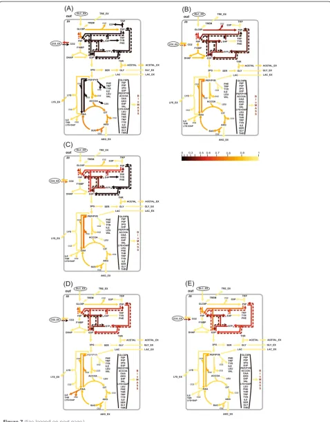
(seeAdditional file 3: Table SF-3.6 for details). The flux spe-cificity of the ηγ(ui) function for the determined me-tabolic model was subsequently shown to be primarily dependent on the applied labeled tracer (see Figures 7 and 8). Indeed, the high resolution of one set of fluxes (e.g., v3: GLC6P →FR F6P; θ4: F6P →R GLC6P; v25:
3PG→F SER; θ26: SER→F GLY + MTHF, with values of η0:95ð Þui ∈½0:65;0:96) and the low resolution of another set of fluxes (e.g.,θ22: PYR + CO2→FOAA;v23: OAA→F
PYR + CO2;θ31: CO2_EX→RCO2, withη0.95(ui) = 0) are
rather typical for experiments using [1-13C]-glucose as the labeled tracer (Figure 7 (A), Figure 8: Column 1). The fol-lowing indication of the η-function emphasizes the type of tracer used and the SLE- or PLE-based character of the provided13C-MFA:
η
0:95u
i;
½
1
−
13C
SLE
.
Concerning the tracer-specific values ofηγ(ui), it was in-teresting to estimate the sensitivity of this function, which is dependent on flux variances, in the case of five simu-lated SLEs with the same tracer. The corresponding calcu-lations were provided for 5 independent SLE with earlier simulated MIDs and the measured effluxes with the Νð0;σmeaÞ normally distributed random errors (Additional file 3: Table SF-3.6 (Exp.3.1-Exp.3.5)). These data are sum-marized in Additional file 2: Figure SF-2.5. The calculated mean-doubled measured specific variances did not exceed 0.02 for nearly all fluxes, and they therefore practically did not change the tracer-specific profile of the η -function. The summarized values of the η-function for all fluxes, (Ση(0.95)([1−13C]SLE))k, which were calculated for each flux
from k= 1, 2,…, 5 SLEs, varied in a rather narrow range (between 37.9 and 38.5). Considering the total number of fluxes (equal to 51) for the assumed metabolic model and the detected measurement-dependent sensitivity of the η -function, if the difference between the Ση(0.95)
Figure 7(See legend on next page.)
Shupletsovet al. Microbial Cell Factories2014,13:152 Page 13 of 25
precision. Certainly, the value of Ση(0.95) could be
con-sidered only as a general, conditional measure of flux resolutions in the investigated network: some metabolic branches could be resolved better, and other branches– worse in different experiments with, perhaps, equal values of summing normalized flux precision functions. So, only the value of theηγ(ui) -function could be con-sidered as the absolute measure of theui-flux resolution efficiency that could be compared with other LEs per-formed with the same metabolic model.
The necessity of a comprehensive statistical analysis of the NLLSP solution
In the present study, the results of the13C-MFA included the set of estimated fluxes, the goodness-of-fit of the model’s adequacy, and the confidence intervals of fluxes, in accord with the recently recommended publishing guidelines [70]. As shown in Additional file 1:SF-1.4., the comprehensive goodness-of-fit analysis had to consist of theχ2-mediated testing of theΞ(θ) objective function at the point of convergence,θ⌢, and confirmation that the indi-vidual weighted residuals used as the summands of this function wereΝð0;1Þdistributed. The solution of the con-strained NLLSP was considered statistically acceptable only if all of the tests were successfully passed.
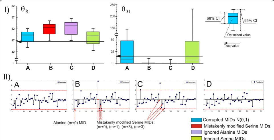
In this report, an example is presented in which the mistaken flux parameters could be assumed when the statistical analysis of the obtained solution was partially provided but to an insufficient extent. Let us analyze the first from five earlier describedin silicoexperiments with 99% [1-13C]-glucose as a tracer (see Table 1 (Exp_3.1)). The“contribution matrix”(see Additional file 1:SF-1.5),
CM;dimðCMÞ ¼ðnwÞ, was computed at the true point, u(θtrue), as an important component of the flux statistics (Additional file 3: Table SF-3.12). It is known [28] that the (CM)ijelements of this matrix indicate the relative importance of the variance of the j-th measure-ment to the local variance of thei-th flux. As can be ob-served in Additional file 3: Table SF-3.12, the variances of the“serine”MIDs demonstrated the high importance of the flux resolution among MS measurements; all matrix columns corresponding to the SER mass isotopo-mers showed rather high sums of their elements. The
variances of these“serine”(“SER”) MIDs significantly in-fluenced the resolution of several fluxes (θ8;θ22;v23;θ31) for the following reactions: GLC6P→FP5P + CO2; PYR + CO2→FOAA; OAA →F PYR + CO2; and CO2_EX →R CO2, respectively. The new set of“experimental data”was generated in the following fashion: the measured effluxes and all MIDs, except for“SER”MIDs, were considered as in the previously analyzed example. The“SER”MIDs were modified as in the case of “poor” resolution of the SER-390 (m + 0) MID, which exhibited an unknown by-product that increased the value of the corresponding SER peak to +4.5%. Due to the necessity of normalizing all SER-isotopomers, the applied modification resulted in a proportional decrease in the other SER MID portions; therefore, the SER-390 MIDs were modified from (m + 0)/ (m + 1)/(m + 2)/(m + 3) = 0.443/0.357/0.140/0.042 (in the previously described example) to a ratio of 0.463/0.344/ 0.135/0.040.
This “mistakenly” modified set of “experimental data” was used to generate the newly constrained NLLSP. A unique solution, corresponding to the minimal values of theΞ=Ξ(θ) objective function with the empty null space of theJf(θ) matrix evaluated at the new point of convergence,
θ¼θ⌢new, was found. Moreover, the value of Ξð⌢θnewÞ was in the χ2 -statistically acceptable interval (see Table 1
(Exp_4.1)). Simultaneously, the parameters obtained for several fluxes did not coincide with the true flux values even in the range of their confidence intervals. Among them there were fluxesθ8andθ31(Figure 9 (I - B)) which
exhibited variances that were essentially determined by SER MID measurements. The fact that the obtained flux param-eters were incorrect could be established only at the stage of normality distribution testing of the weighted residuals; three variance-weighted residuals corresponding to “ SER-390”MIDs and one corresponding to“alanine (ALA)-260” were shown to be located outside of the 95% confidence interval (Figure 9 (II-B)). According to the general recom-mendation presented inSF-1.4, improvement of the solu-tion statistics could be achieved due to the excision of the “prominent”residuals from the expression for the objective function followed by the repeated solution of the con-strained NLLSP with the partially truncated Ξ function. Two alternative NLLSPs were generated where ALA or SER (See figure on previous page.)
Figure 7The values of the normalized flux precision function in the different parts of the assumed metabolic network depend significantly on the applied tracer(s).The results of flux estimation:(A)SLE using 100% [1-13C]-glucose as the tracer; and from PLEs consisting of:(B)5 LEs using different mixtures of [U-13C]/[U-12C]-glucose in each LE, with 20%, 35%, 50%, 65%, or 80% [U-13C]-glucose;(C)5 LEs using partially optimized mixtures of [1-13C]/[U-12C]/[U-13C] glucose for the separate minimization of the approximated variances of the
θ10,θ12,θ14,θ22,θ31free fluxes in each LE;(D)3 LEs using 100% [1-13
MIDs were excluded from the“experimental data”set. Pa-rameters obtained after solution of the NLLSP with ignored “ALA-260”MIDs did not coincide with the true flux values
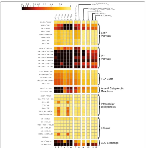
in the range of their confidence intervals (Figure 9 (I-C)). Moreover several variance-weighted residuals still located outside of the 95% confidence interval including that of Figure 8Normalized flux precision functions for all fluxes are presented in the form of color-scored squared diagrams for the different tracers used for simulations.The columns correspond to the following labeling experiments:1,2,….,6−SLEs with 100% [i-13C]-glucose as a tracer, wherei= 1, 2,…, 6, respectively;7−an SLE with a generally optimized (minimumD-value) mixture of [U-13C]65%/[U-12C]35%-glucose;8−a PLE consisting of 5 LEs with different mixtures of [U-13C]/[U-12C]-glucose in each LE, where the fraction of [U-13C]-glucose was 20%, 35%, 50%, 65%, or 80%;9−a PLE consisting of 5 LEs with partially optimized mixtures of [1-13C]/[U-13C]/[U-12C] glucose for separate minimization of the approximated variances of theθ10,θ12,θ14,θ22,θ31free fluxes in each LE;10−a PLE composed of 3 LEs using 100% [1-13C]-, [3-13C]-, or [4-13C]-glucose as the tracer;11−a PLE consisting of 6 LEs, where all singly labeled isotopomers of glucose, as in1–6, were used as tracers;12−a PLE composed of 6 LEs, including 3 of the LEs used in10, corresponding to partial optimization forθ4andθ12,θ14,θ22andθ31, and 3 other LEs using the partially optimized mixture of [1-13C]/[3-13C]/[4-13C]-glucose to minimize the approximated variances of theθ8,θ10,θ
26free fluxes.
Shupletsovet al. Microbial Cell Factories2014,13:152 Page 15 of 25
“SER-390”(Figure 7 (II-C)). In contrast, the proper statisti-cally acceptable solution was obtained for NLLSP with ignored“SER-390”MIDs, which coincided with true fluxes in the range of the determined flux confidence intervals (Figure 9 (I-D) and (II-D)). Thus,“incorrect flux parameters” could be assumed if test for normality of variance-weighted individual residual distribution is ignored. Certainly, higher negative influence on the proper flux estimation could be assumed ifχ2-statistically unacceptable solution is obtained. Analysis of variance-weighted residuals plot followed by step by step exclusion substances with prominent residuals, as described in the example, could help to identify“incorrect measurements” and, perhaps, to obtain statistically accept-able solution with correctly estimated parameters.
It is obvious that measured MIDs and effluxes’ param-eters are completely separate categories of experimental data that could not be trivially compared. It is well established [3] that labeling experiments are performed to resolve internal fluxes, even parallel and cycle path-ways, and reversible reactions, which cannot be resolved on the basis of measured effluxes. Nevertheless, the vari-ances of the measured effluxes could provide the most significant influence on the resolution of some fluxes, as could be seen from the values of the corresponding (CM)ij elements in the Additional file 3: Table SF-3.12.
Thus, generally, it is desirable to execute the efflux mea-surements with the highest possible accuracy to decrease the variances and totally improve the flux resolution. One of the interesting step in this direction has been done recently when the authors tried to increase the measurement accuracy for an efflux corresponding to quantifying biomass composition due to exploiting of the high-precision GC-MS technique [71]. Unfortunately, in many cases, the efflux measurements as the stage of label-ing experiment have received much less attention than the more glamorous stages of the subsequent highly-precised MS-based measurements.
Simulations of LEs with [U-13C]-glucose as a tracer
A uniformly13C-labeled isotopomer of glucose, [U-13 C]-glucose, is often used as a tracer in 13C-MFA. In the present study, new sets of “experimental data” were generated for the same metabolic model when different relative amounts of [U-13C]-glucose (20%, 35%, 50%, 65%, and 80%) mixed with non-labeled ([U-12C]) glucose were used as the sole carbon source (Additional file 3: Table SF-3.8).
fitting to the single metabolic model (see Table 1
(Exp_5.1-Exp_5.5; PLE_1) and Additional file 3: Table SF-3.8). As shown by the presented data, the SLE-based13C-MFA resulted in values between 35.4 and 40.4 for the Ση(0.95)([U−13/12C]SLE) function (Additional file 3: Table
SF-3.8). Again, a set of tracer-specific fluxes that possessed rather high values of the η-function could be detected (at least more than in the case of exploiting [1-13C]-glucose as a tracer), e.g., θ22: PYR + CO2 →F
OAA;v23: OAA→FPYR + CO2;θ31: CO2_EX→RCO2.
The PLE-based 13C-MFA of experiments using [U-13/12 C]-glucose as the carbon source actually improved the resolution of all fluxes estimated in the corresponding SLEs,Ση(0.95)([U−13/12C]PLE) = 42.4. Moreover, the
tracer-specific behavior described in relation to SLEs was reproduced in the PLE. The colored scheme presented in Figure 7 and the diagram in Figure 8 correspond to the cal-culated values of theη-function for all fluxes obtained in different experiments, illustrating this fact and demonstrating that optimization of the experimental design is necessary to increase the precision of the targeted fluxes [19,49,54,62].
Optimal design for LEs using mixtures of [U-13C]-, [1-13C]-, and [U-12C]-glucose isotopomers
To achieve the best flux resolution in an LE employing a mixture [U-13C]-, [1-13C]-, and [U-12C]-glucose isotopo-mers as the carbon source, optimization of the experimen-tal design could be performed according to the method proposed by Möllney et al. [19]. In their study, the com-parison of different designs was based on an evaluation of
D-factor values [72], i.e., the squared volumes of the flux confidence ellipsoids for a given confidence level. Accord-ing to [19] and usAccord-ing the notations introduced in the present study, the squared volume of the p-dimensional confidence ellipsoid for free fluxes, which was evaluated at the point of convergence,θ¼⌢θ, could be obtained (up to a constant that does not depend on designed parameters) using the following expression:
Dðminput;mmea;σmea;⌢θÞ ¼ detΣ⌢θðminput;mmea;σmea;⌢θÞ
¼ det½HSSRð⌢θÞ−1
ð5Þ
whereΣ⌢θis a covariance matrix of the free fluxes estimated according to linearized statistics (see Additional file 1:
SF-1.5.) and to the approximation of this matrix by the
in-verse Hessian matrix presented in Eq. (A2−10) Additional
file1:SF-1 Appendix 2. Specifically, the last equality from
Eq. (5) was used for computation of theD-factor. Accord-ing to a previous suggestion [19], the use of the value of the 2ppffiffiffiffiD
parameter, which can be interpreted as an aver-age length of the confidence interval of estimated fluxes, is more suitable. As noted previously, the confidence
ellipsoid volume estimation provided by Eq. (5) holds
true within some vicinity of the predefined pointθ¼⌢θ
and can change due to a shift in that point [19].
Be-cause the true values of the free fluxes were known for our artificial metabolic model, the optimization of the experimental design, which was dependent on the tested 13
C-labeled tracers, was significantly simplified and was based on the computation of the determinant of the in-verse Hessian matrix evaluated at the point θ=θtrue. In practice, when the true flux values are not knowna priori, they are assumed, for example, from data in the literature,
FBA or even from 13C-MFA performed on the basis of a
rather inexpensive label [37,63]. In some cases, a second round of experimental design optimization is necessary if the proposed flux distribution is far from the feasible point of convergence obtained in a planned labeling experiment [73,74]. In the present study, all of the new experimental designs were compared with the reference design (SLE
with 99% [1-13C]-glucose as the tracer) using the value
of the p2pffiffiffiffiD
parameter. In addition to the “general
optimization” achieved due to the minimization of the
relative value of the average confidence interval length:
Dopt minput;mmea;σmea;θtrue
¼ min
minput−feasible
ffiffiffiffiffiffiffiffiffiffiffiffiffiffiffiffiffiffiffiffiffiffiffiffiffiffiffiffiffiffiffiffiffiffiffiffiffiffiffiffiffiffiffiffiffiffiffiffiffiffiffiffiffiffiffiffiffiffiffi
Dnew minput;mmea;σmea;θ true
ð Þ
Dref mref;mmea;σmea;θ true
ð Þ
2p s
ð6Þ
“partial optimization” could be obtained as a result of minimization of the standard deviation of the targetedθi free flux, which, in turn, was approximated as the square root of the corresponding diagonal element of the Σθ⌢ matrix:
min
minput−feasible σ θtrue lin
i¼minputmin−feasible
ffiffiffiffiffiffiffiffiffiffiffiffiffiffiffiffiffiffiffiffiffiffiffiffiffiffiffiffiffiffiffiffiffiffiffi
HSSRðθtrueÞ
½ −1
ii
q
ð7Þ
The results of the corresponding computations per-formed using the special subprograms implemented in OpenFLUX2 software are presented in Additional file 2: Figure SF-2.6. According to the provided calculations, “general optimization” required the use of a mixture of [1−13C]78 %/[U−13C]22 %glucose isotopomers in the SLE (Additional file 2: Figure SF-2.6 (A)). Interestingly, these
D-factor-mediated optimized tracer compositions were extremely close to the [1−13C]80 %/[U−13C]20 % -labeled mixture of glucose that has been used without any cal-culations to achieve a rather high flux resolution in other experimental systems (e.g., Escherichia coli-based systems [48], in particular). In contrast, the sameD- criterion-based approach resulted in another optimal mixture of the same glucose isotopomers ([1−13C]48 %/[U−13C]40 %/ [U−12C]12 %) when some modifications differed in the
Shupletsovet al. Microbial Cell Factories2014,13:152 Page 17 of 25
metabolic model of the L-lysine-producing C. glutami-cumstrain applied in the present study, and plans were made to obtain another set of measurements [19].
According to the provided computations, “partial optimization,” i.e., the optimal resolution of different tar-geted free fluxes, had to be achieved in the SLEs with the distinguished mixtures of the same glucose isotopomers (e.g., see Additional file 2: Figure SF-2.6 (B - F)). Several of the proposed optimal designs (e.g., see Figure 10 (I)) were realized using computer simulations, and the set of experimental data was generated, followed by a search of the solution for the corresponding con-strained NLLSP. One of the simulated SLEs was per-formed using the “generally optimized” mixed tracers, five others employed the “partially optimized” mixtures,
and five experiments were performed with the randomly chosen mixture of [1−13C], [U−13C] and [U−12C] glucose isotopomers (“randomly mixed”) as the tracers. As shown in the presented results (Additional file 3: Table SF-3.9), the SLE with “generally optimized” conditions resulted in Ση(0.95)([1−13C]78 %[U−13C]22 %SLE) = 38.4, with “partially optimized” conditions– Σηð0:95ÞðParOptSLEÞ∈½36:0;38:7, and with“randomly mixed”tracers–Σηð0:95ÞðRanMixSLEÞ∈
35:2;39:1
½ . It has to be especially noted, that SLEs with the higher calculated values than Ση(0.95)= 38.4 was
detected here, and among described earlier (see, final Additional file 3: Table SF-3.11), and so“general”and/or “partial” optimizations does not result in maximization of the sum of normalized precision functions for all fluxes, Ση(0.95). Simultaneously, the free fluxes, θi, that
Figure 10Experimental design studies for the identification of mixtures of [1-13C]/[U-12C]/[U-13C]-glucose isotopomers for“general” optimization or for the best resolution (“partial”optimization) ofθ31,θ14,θ22fluxes (I), results of these flux estimations (II) obtained through13C-MFA of the simulated SLEs (A–F) or PLEs (G) with the mentioned mixed tracers: A−SLE, 0/50/50, %% (partially optimized forθ12); B−SLE, 10/44/46, %% (partially optimized forθ22); C−SLE, 13/0/87, %% (partially optimized forθ31); D−SLE, 66/0/34, %% (partially optimized forθ14); E−SLE, 89/0/11, %% (partially optimized forθ10); F−78/0/22, %% (generally optimized); G−PLE consisting of five LEs using the same tracers as in A–E for each experiment (red 68%CIboxes); (III) the normalized flux precision function values for the confidence level ofγ= 0.95 computed for these (A–G) experiments.Green 68%CIboxes in