M E T H O D O L O G Y A R T I C L E
Open Access
Deriving movement properties and the
effect of the environment from the Brownian
bridge movement model in monkeys and birds
Kevin Buchin
1*, Stef Sijben
2, E Emiel van Loon
3, Nir Sapir
4, Stéphanie Mercier
5, T Jean Marie Arseneau
6and Erik P Willems
6Abstract
Background: The Brownian bridge movement model (BBMM) provides a biologically sound approximation of the movement path of an animal based on discrete location data, and is a powerful method to quantify utilization distributions. Computing the utilization distribution based on the BBMM while calculating movement parameters directly from the location data, may result in inconsistent and misleading results. We show how the BBMM can be extended to also calculate derived movement parameters. Furthermore we demonstrate how to integrate environmental context into a BBMM-based analysis.
Results: We develop a computational framework to analyze animal movement based on the BBMM. In particular, we demonstrate how a derived movement parameter (relative speed) and its spatial distribution can be calculated in the BBMM. We show how to integrate our framework with the conceptual framework of the movement ecology
paradigm in two related but acutely different ways, focusing on the influence that the environment has on animal movement. First, we demonstrate ana posterioriapproach, in which the spatial distribution of average relative movement speed as obtained from a “contextually naïve” model is related to the local vegetation structure within the monthly ranging area of a group of wild vervet monkeys. Without a model like the BBMM it would not be possible to estimate such a spatial distribution of a parameter in a sound way. Second, we introduce ana prioriapproach in which atmospheric information is used to calculate a crucial parameter of the BBMM to investigate flight properties of migrating bee-eaters. This analysis shows significant differences in the characteristics of flight modes, which would have not been detected without using the BBMM.
Conclusions: Our algorithm is the first of its kind to allow BBMM-based computation of movement parameters beyond the utilization distribution, and we present two case studies that demonstrate two fundamentally different ways in which our algorithm can be applied to estimate the spatial distribution of average relative movement speed, while interpreting it in a biologically meaningful manner, across a wide range of environmental scenarios and ecological contexts. Therefore movement parameters derived from the BBMM can provide a powerful method for movement ecology research.
Keywords: Brownian bridge movement model, Movement speed, Spatial distribution, Home range utilization, Migratory flight behaviour
*Correspondence: [email protected]
1Department of Mathematics and Computer Science, Technical University Eindhoven, Eindhoven, The Netherlands
Full list of author information is available at the end of the article
© 2015 Buchin et al. This is an Open Access article distributed under the terms of the Creative Commons Attribution License (http://creativecommons.org/licenses/by/4.0), which permits unrestricted use, distribution, and reproduction in any medium, provided the original work is properly credited. The Creative Commons Public Domain Dedication waiver
Background
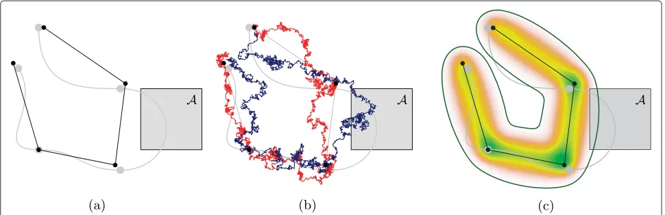
Modelling movement as a stochastic process provides means to estimate paths or location distributions when observations were not recorded continuously. This per-spective is, however, often overlooked when analyzing movement based on discrete observations. For instance kernel-density estimation, which is frequently applied to movement data, does not take temporal autocorrelation into account. It is used for home-range estimation [1, 2] when the sampling rate is sufficiently low so that indepen-dence between observations can reasonably be assumed. Similarly, home range estimation based on minimum convex polygons [3] also ignores the actual movement between different locations. In other uses of movement data, locations are interpolated under the assumption of a linear movement path between observations [4]. This assumption is unrealistic except for densely sampled data, and can lead to wrong conclusions on sparser data as illustrated in Fig. 1(a).
Stochastic models like state-space models [5–7] and the
Brownian bridge movement model (BBMM)[8–12] have been successfully applied for estimating the movement path and intensity of space use based on discrete loca-tion data. In this paper we explicitly focus on the BBMM (but see online Additional file 1 for a more elaborate dis-cussion of the similarities and differences between the BBMM and state-space models). The BBMM takes the movement of animals into account to calculate space use patterns. It does so making relatively few assumptions, yet still making biological sense in that its parameters reflect real properties of the relocation data: measure-ment accuracy and –in a way– speed and directionality of movement. The assumption underlying the BBMM is that the entity exhibits purely random (i.e., Brownian) motion. In a typical scenario in which the BBMM is applied, we have multiple location measurements and are interested to infer the location at times in the interval between two consecutive measurements. Therefore, we condition Brownian motion on the measured locations at the observation times. Such a conditioned Brownian motion is called a Brownian bridge, which is illustrated in Fig. 1(b–c). The BBMM has the desirable property of being able to take measurement uncertainty into account, usually by assuming that this uncertainty follows a Gaussian distribution around a given relocation point (which is an appropriate assumption for e.g. relocations obtained from GPS-telemetry [13]). In contrast to pure Brownian motion, however, additional Gaussian noise results in a process that is not Markov [14].
The use of the BBMM in the context of movement ecol-ogy was proposed by Bullard [8] and Horne et al. [9] and is defined by the measurement error and the diffusion coefficient, which relates to an organism’s mobility. Horne et al. propose to compute the diffusion coefficient using
maximum likelihood estimation, thereby explicitly assum-ing homogeneous movement throughout an entire tra-jectory. However, as movement parameters change over time, it is biologically more realistic to allow the diffu-sion coefficient to vary. Kranstauber et al. [10] use the Bayesian information criterion to detect changes in the movement state of an organism, and use this to vary the diffusion coefficient over time. Bivariate Gaussian bridges factorise diffusion into a parallel and an orthogonal com-ponent [11]. A related algorithm is the Biased random walkproposed by Benhamou [15]. In his study the sam-pling density is increased using linear interpolation and then kernel density estimation is used at the resulting set of locations. Overall, these methods provide a more advanced estimate for the location distribution in rela-tion to using a fixed diffusion coefficient, because they are more dynamic or segment-specific.
The BBMM has so far been exclusively used to com-pute utilization distributions. The analysis of movement, however, often does not ask for location as such, but rather focuses on derived movement parameters like rel-ative speed, or more complex analysis tasks like similarity estimation between trajectories. In recent work Buchin et al. [16] show how to derive such parameters and how to perform fundamental analysis tasks under the assumption of a BBMM. Since their paper focused on the techni-cal side of mathematitechni-cally deriving the corresponding parameters, they assumed that movement takes place in a featureless space, not taking into account the external and internal factors that govern organismal movement.
Clearly though, these factors are essential for a proper biological understanding of animal movement. Nathan et al. [17] proposed a paradigm, which incorporates four basic components that affect a movement path: exter-nal factors, the interexter-nal state of the moving organism, its navigational capacity and its motion capacity. Getz and Saltz [18] present a framework for generating and ana-lyzing movement paths using this paradigm, which can be used to generate movement paths by simulation and to segment movement paths by state-space methods. It does not, however, deal with the interpolation of location observations.
Fig. 1Linear interpolation compared to Brownian bridges. Linear interpolation compared to Brownian bridges. In this example the movement path is shown in gray and the location data as black dots connected by straight line segments.aLinear interpolation would incorrectly report that the movement path does not traverse the areaA.bTwo realizations in the BBMM, one of which traversesA.cUtilization distribution (density indicated by shading) and 99 % volume isopleth, which intersectsA
an absolute measure. Further, we note that in our frame-work calculations are performed per bridge, and for any given bridge only the two adjacent observations are used. While this is in line with the work of Horne et al [9], this does not account for sequence of observations being not Markov [14] in the presence of measurement errors.
In the Results section we first discuss how various fac-tors influencing a movement path can be incorporated in such an analysis. We differentiate between two related but acutely different approaches to do so. The first approach takes factors into accounta posteriori, that is, they do not influence the movement model but are used to biologi-cally interpret its outcome. The second takes factors into account a priori, that is, factors influence a key model parameter (the diffusion coefficient), and thereby the esti-mation of the movement path and derived properties.
We demonstrate our framework on data of two species with distinctly different movement.
We apply thea posterioriapproach in a case study on how the movement speed of vervet monkeys (Chlorocebus pygerythrus) within a monthly ranging area is related to local vegetation density, whereas for thea prioriapproach we look at the flight mode of European bee-eaters (Merops apiaster) during migration.
Results and discussion
Computational aspects of the movement ecology framework
Organismal movement can be perceived as the outcome of the interaction between four key biological compo-nents: factors external to the organism, the organism’s internal state, its navigational capacity, and its motion capacity [17]. In this paper we focus on external fac-tors and consider two ways in which their relation to
the movement can be investigated. First we consider the case in which the components do not affect the compu-tation of the BBMM, but instead are used a posteriori
to biologically interpret its outcome. Second, we use the componentsa priorito dynamically modify a key parame-ter of the BBMM, the diffusion coefficient. This approach is in general more difficult to handle computationally. The aspect which dictates this difficulty is the degree of spatial dependence of the components. If they are independent of space, possibly conditional on time or some measure-ment (e.g. behaviour, which may be identified in the basis of a short acceleration signal) [19]), it can be handled in an analytical movement model. In contrast, if a factor is especially spatially dependent (e.g. a highly heterogeneous habitat), an explicit simulation of the spatial trajectory is required. This would effectively imply a multitude of simulations because we are interested in conditional dis-tributions. If a factor is only varying relatively little over the length of a trajectory segment (e.g. atmospheric vari-ables like wind or thermal convection), it is possible to make a quasi-steady state assumption and consider it as constant within a local spatial domain. This makes it much easier to handle spatial dependency in a BBMM.
In the following, we elaborate on the various settings at the hand of two case studies. In the first study the external factor (vegetation density) is given as raster data and has a strong spatial dependency. In this setting the
a posteriori approach is applicable. The challenge here is to compute a spatial distribution of average speed. In the second study the external factor (atmospheric condi-tions) is given along the movement path and therefore the
Movement speed of vervet monkeys – thea posteriori approach
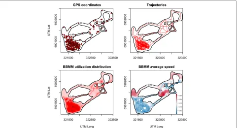
In the first case study, we apply our framework to inves-tigate local differences in the movement speed of a wild group of free-ranging vervet monkeys within their rang-ing area over a 1 month period. Movement data were obtained from a GPS logger, deployed on a single adult female within the group and programmed to collect coor-dinates at hourly intervals during the animals’ daily activ-ity period. In total, 465 relocations were collected this way (Fig. 2a), representing 31 daily trajectories (Fig. 2b). The GPS data is provided as Additional file 2.
We first employ our implementation of the dynamic BBMM to calculate the monthly utilization distribution of the monkeys and delineate their ranging area by a 99 % volume isopleth (Fig. 2c). This revealed the monkeys used an area of 1.3 km2 over the observation period. Then we investigate how speed estimates from this dynamic BBMM relate to the external environment in which the animals are moving. We hypothesize that the monkeys travel faster in the more open, less densely vegetated areas of their range (due to greater exposure to predators and lower food availability), and slower in those areas in which the vegetation is more lush (more safety and food). We investigate this hypothesis by relating our average speed estimate (calculated over 5 minute time intervals; Fig. 2d) to local vegetation density, proxied by a high resolution
(0.50×0.50 m2) Normalized Difference Vegetation Index (NDVI) image (see Methods section). High NDVI values correspond to high vegetation density, whereas low val-ues reflect sparse vegetation. We thus predict a negative association between the average movement speed of the monkeys and local NDVI values.
To statistically test this prediction, we generated 1000 random sample locations throughout the monthly range of the animals and extracted both local NDVI and speed estimate values. Since data exhibited significant levels of spatial autocorrelation (as indicated by inspections of Moran’s I values and correlograms), statistical sig-nificance of the association between local vegetation density and speed of movement was assessed using geo-graphically effective degrees of freedom [20]. This anal-ysis revealed a significant, negative correlation between local NDVI-values and BBMM-estimated average rela-tive speed (rPearson = −0.213,F(1, 975.68) = 46.15,p <
0.0001), in line with our biological expectations. We also performed the same analysis using only one diffu-sion coefficient (i.e., non-dynamic BBMM), which also showed a significant, negative correlation (rPearson =
−0.175,F(1, 150.27)=4.78,p=0.03).
Migration of European bee-eaters – thea prioriapproach
The European bee-eater is a species that uses both flapping and soaring-gliding flight during its migratory
movement. In this case study we use the relationship between atmospheric conditions and flight mode in this species [21, 22] to construct a biologically informed BBMM that generates estimates of flight speed and trajec-tory uncertainty over different segments of the movement path, depending on likely flight-mode. Even though the influence of atmospheric conditions on the movement path (mediated by flight mode) has previously been inves-tigated [22–25], this information has not yet been inte-grated into a movement model for the European bee-eater. We hypothesize that soaring-gliding flight is character-ized by an overall less straight, more tortuos path because in this flight mode birds may rely on the spatial variabil-ity of convective thermal intensvariabil-ity. Since soaring-gliding birds may actively select to circle in strong thermals that are not necessarily found in the exact direction of their flight destination, their path may be less direct or straight. Additionally, since migration speed scales differently with bird size for flapping and soaring-gliding flight modes, for relatively small birds like the European Bee-eater (mean body mass of 56 g [22]), it has been suggested that soaring-gliding will be slower than flapping flight [26]. To inves-tigate these hypotheses we calculate and compare the diffusion coefficients and average flight speeds for the two flight modes using the BBMM.
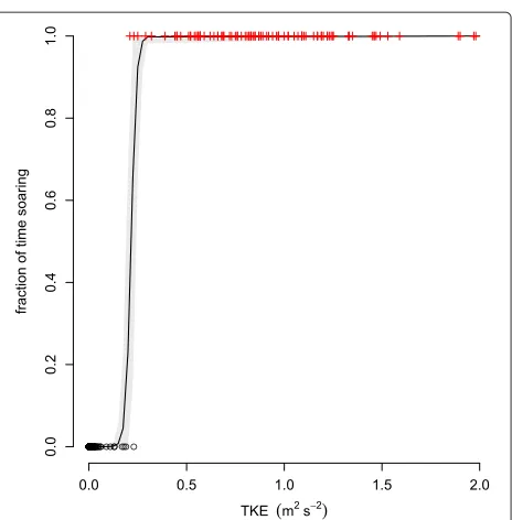
The data set consisted of 91, 141 and 94 segments char-acterized by flapping, mixed and soaring-gliding flight modes respectively (see [22] for additional details). The data was collected by radio telemetry, resulting in an irreg-ular measurement frequency of approximately 6 minutes (343 seconds with standard deviation of 547 seconds). The data set is provided as Additional file 3. We use a model to predict the fraction of time spent on soaring-gliding flight as a function of atmospheric conditions (most notably, the magnitude of the Turbulence Kinetic Energy, or TKE). After calibration, our model classified the animals’ flight mode with an overall error rate of 1.1 %. This model has the following form:
ea·TKE−b
1+ea·TKE−b,
where the value (with 95 % confidence bounds) for param-eter a is 74 (25 - 227), and for parameter b is 16 (5 -50). Figure 3 shows the shape of this model as well as its predictive uncertainty.
We selected the movement segments with the pure flapping and soaring-gliding flight modes and applied the maximum likelihood estimation by Horne et al. [9] separately to these. This resulted in estimated diffusion coefficients for flapping as 2965 m2/s and 4505 m2/s for soaring-gliding. This confirms our hypothesis that soaring-gliding is associated with a more tortuous flight path. The fact that this hypothesis could be investigated empirically on the basis of such sparse and irregularly
Fig. 3Logistic function. The logistic function describing the fraction of time the birds flew using soaring-gliding as a function of turbulence kinetic energy (TKE). The grey-shaded range is a 0.95 confidence interval
sampled data is a distinct advantage of our approach over previous BBMM-based methods that, moreover are restricted to calculations of space use only. The difference in diffusion coefficients between the two flight modes is illustrated in Fig. 4. In this figure, the spatial distributions of two individuals are shown along with their flight mode. The movement path is clearly wider for segments with soaring-gliding flight than for those with flapping flight, and, to our knowledge, this aspect of flight mode on the migratory track has not yet been described elsewhere.
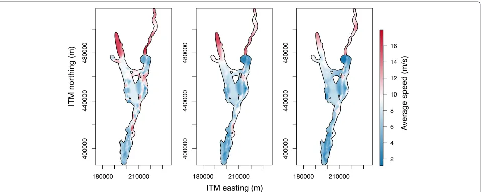
We calculated the movement speeds using our BBMM over 5 minute instances. Reasons for this resolution were the resolution of the original observations (approximately 6 minutes on average) and the fact that autocorrelation is very limited at this 5 minute resolution. At this resolution we found that the average relative cross-country speed for flapping flight was 9.7 m/s, while in soaring-gliding flight it was 8.5 m/s, a significant difference of 1.2 m/s (Welch two-sample T-test; 95 % confidence-interval: 0.91 - 1.56). The variance of relative cross-country speed for flapping flight was 16.2 m2/s2and 7.1m2/s2for soaring-gliding flight, a ratio of 2.30 (significant according to a 2-sided F-test; 95 % confidence-interval: 2.05 - 2.60).
190000 200000 210000 220000
430000
440000
45000
0
46000
0
470000
ITM easting (m)
ITM nor
thing (m)
5:30 4:21
11:25 2:47
1:51 1:47
5:26 4:57
6:20 1:12:02
2:44 2:12 11:55 2:06
4:55
0:17 4:45
2:07 2:28
170000 200000 230000
380000
420000
460000
500000
ITM easting (m)
ITM nor
thing (m)
Fig. 4Changing diffusion coefficients. Two examples of the effect of a changing diffusion coefficient on the predicted trajectory. The coloured line is interpolated linearly between measured locations, where blue means a low diffusion coefficient mainly flapping flight), and red means a high diffusion coefficient (mainly soaring/gliding flight). The contours indicate the 90 % and 99 % volume isopleths based on the trajectory. In the example to the right the time passed between two measurements is indicated. A larger diffusion coefficient results in a wider contour. For instance, of two bridges of similar duration (4:55 and 4:57 minutes and length the red bridge has a wider contour than the blue
intense and this may have influenced our calculations that dealt only with the cross-country flight speed. Figure 5 shows the spatial distribution of average cross-country speed relative to three different time scales. We further note, that the speed variability within the soaring-gliding flight mode could be resolved if fine-resolution obser-vations (e.g. < 30 seconds) would be available. In that scenario, the variability in speed differences which is now implicit in the higher diffusion coefficient for that mode would become explicit through a higher variance in speed (at fine resolutions) for the soaring-gliding flight mode.
We further note that the calculated speeds depend on the diffusion coefficient, the displacement between two observations and the chosen time scale; therefore –as is the case here– a higher diffusion coefficient does not necessarily imply higher speed.
Conclusions
We demonstrated how the Brownian bridge movement model can be extended to compute the spatial distribu-tion of derived movement parameters, such as relative speed, and used two case studies to illustrate different
180000 210000
400000
44000
0
480000
180000 210000
40000
0
440000
480000
180000 210000
400000
44000
0
480000
2 4 6 8 10 12 14 16
A
vera
g
e speed (m/s)
ITM nor
thing (m)
ITM easting (m)
ways (thea posteriorianda prioriapproach) in which our computational framework can integrate environmental factors with the BBMM. In both case studies our frame-work provided meaningful biological insights that could not have been obtained previously from the BBMM.
In the first case study, we used our framework to first calculate the utilization distribution and monthly rang-ing area of a group of vervet monkeys. Subsequently, we could analytically confirm the hypothesized relationship between the local average speed with which the animals traverse their ranging area to local vegetation density. Cor-relating local average speed to vegetation density required BBMM-based calculations novel to our paper, specifically an estimation of the spatial distribution of speeds. It would be interesting to see how a correlating variable could be used to estimate diffusion coefficients of a BBMM directly, which however seems like a computationally challenging task; this could mean that ana posterioriapproach would be used as inspiration to apply ana prioriapproach.
In the second case study, we used existing knowledge about the relationship between atmospheric conditions and flight mode of migrating European bee-eaters, to evaluate whether different flight modes result in differ-ent average cross-country flight speed and tortuosity of the movement path. This was not possible in previous studies [21, 22] due to varying sampling intervals. Here, however, we first fit a biologically informed BBMM, which then enabled us to demonstrate that soaring-gliding flight involves higher variability in route straightness and lower flight speeds than flapping flight. Our work therefore adds a novel perspective to bee-eater biology, and the novel findings –not discovered by the traditional approaches– demonstrate the usefulness of the new approach.
Both case studies heavily rely on the ability to not only estimate the spatial distribution of an animal but to also estimate derived movement parameters and their spatial distribution based on the BBMM – an application of the BBMM unique to our work. We note that many of the conceptual questions we address for the BBMM –like the use of spatial distributions of movement parameters to integrate environmental factors into the analysis– are also relevant to other movement models.
In general, our framework may apply to settings where environmental factors are expected to influence veloc-ity. For terrestrial, aquatic and airborne organisms that could respectively be terrain ruggedness, currents and wind. However, also an organism’s internal state or inter-action with other organisms may (when observations on these variables are available) be incorporated in the anal-ysis. Even though our case studies do not represent all these possibilities, they do demonstrate that the deriva-tion of movement parameters and their spatial distri-bution via BBMM is a powerful method for movement research.
Methods
Methods for computing movement parameters in the Brownian bridge movement model
We first discuss how various movement parameters are calculated in the BBMM and similar models. We then pro-vide details on the specific methods used in the two case studies. The BBMM assumes that an entity exhibits Brow-nian motion between measured locations. A BrowBrow-nian bridge is the distribution of this process conditioned on the locations of both endpoints. To model uncertainty in the measured locations and to avoid a degenerate proba-bility distribution at the time of a measurement, the loca-tions are often assumed to be normally distributed around the measured location. All of the following calculations are performed for individual Brownian bridges and only use the directly adjacent measurements. Note that in the presence of measurement errors the sequence of observa-tions does not satisfy the Markov property [14], and any Brownian bridge actually depends on more than just the adjacent measurements. Thus, we need to assume that the measurement error is small relative to the diffusion coefficient.
If we assume that we have two locationsxi,xi+1
mea-sured at timesti,ti+1with variancesδ2i andδi2+1
respec-tively, the position Xt at a time t ∈[ti,ti+1] follows a
circular bivariate normal distribution with parameters
μ(t) = (1−α)xi+αxi+1,
σ2(t) = (t
i+1−ti)α(1−α)D+(1−α)2δ2i +α2δi2+1.
Here,α = t−ti
ti+1−ti is a variable that linearly moves from 0
to 1 astmoves fromtitoti+1andDis the diffusion
coef-ficient of the Brownian motion, which is often estimated by a maximum likelihood method [9]. When the trajec-tory contains different movement states over time, it may be appropriate to vary the diffusion over time rather than to keep it constant [10].
Given these probability distributions, derived parame-ters such as distance or speed (relative to a time scale) can be determined [16]. These parameters are important building blocks for the detection of many movement pat-terns. We summarize the results on the distributions of these parameters here, for full derivations we refer to [16] and online Additional file 4. Note that the derivation of velocity in [16] does not handle all possible dependencies and is superseded by the derivation in Appendix 1.
If the positions of two animalsAandBat timethave independent circular normal distributions with means
μA(t) andμB(t) and variances σA2(t) and σB2(t) respec-tively, the distance betweenAandBhas a Rice distribution with parameters|μA(t)−μB(t)|and
σ2
A(t)+σB2(t). The average velocity over a time interval [t1,t2] is given by
velocity has a circular normal distribution with mean μ(t2)−μ(t1)
t2−t1 , while the expression for the variance depends on the number of location measurements that were obtained betweent1andt2.
Letts,tiandtf be the time stamps of three consecutive observations with location variancesδ2
s,δ2i andδ2f respec-tively, chosen such thatts ≤ t1 < ti. The observation at
tf is only needed in the calculations ifti < t2 ≤ tf. The variance of the velocity is:
σ2
V(t1,t2)=
⎧ ⎪ ⎪ ⎪ ⎪ ⎪ ⎪ ⎪ ⎨ ⎪ ⎪ ⎪ ⎪ ⎪ ⎪ ⎪ ⎩ δ2 s+δ2i (ti−ts)2 +
1
ti−ts + 1
t2−t1
ift1<t2≤ti, σ2(t
1)+σ2(t2)−2
t
1−ts ti−ts tf
−t2 tf−ti
δ2 i
(t2−t1)2 ifti<t2≤tf,
σ2(t 1)+σ2(t2)
(t2−t1)2 otherwise.
Let μV andσV2 be the parameters of the velocity dis-tribution over a time interval [t1,t2]. Speed (the absolute
value of velocity) over this interval then has a Rice distri-bution with parameters|μV|andσV. The direction of this velocity has a distribution with density
f(γ )=e
−ν2 2
2π + νcosη 2√2π exp
ν2cos2η−1
2
× 1+erf νcos√ η
2
,
whereν = |μV|
σV is the noncentrality of the velocity
distri-bution andη = atan2μV−γ is the angle between the direction of the mean and the direction under considera-tion.
To obtain spatial distributions of speed, we consider the speed over a time interval [t + ts,t+ tf], after fix-ing the position at one timet to a fixed location. If the time interval contains the time at which the position is fixed, i.e. ts ≤ 0 and tf ≥ 0, the position distribu-tions at both endpoints of the interval are independent. The conditioned velocity and speed distributions are then determined from these two distributions. The spatial dis-tribution of speed and the effect of the choice of the time scale ( tf − ts) is illustrated in Fig. 5 by the example of the data used in the second case study.
We do not give the details about these position distribu-tions here, but refer to Appendix 1. Letμs,μf,σs2andσfs represent the respective means and variances of the con-ditioned positions at both endpoints of the interval. Then by independence of the positions the velocity distribution
conditioned onXt=xis given by
Vx;t(t+ ts,t+ tf)=
Xt+ tf −Xt+ ts
tf− ts
∼N μf −μs
tf − ts
σ2 s +σf2
tf− ts 2
.
As discussed before, the speed has a Rice distribution. We determine the average speed at a particular location by computing a weighted average over time of the mean speed. The weight is given by the probability density of the animal’s position at the given time and location. That is,
S(x)= 1
fXt(x)dt
fXt(x)E
|Vx;t(t+ ts,t+ tf)|
dt. (1)
Methods for the analysis of the movement speed of vervet monkeys in relation to their environment
Vervet monkeys are group-living primates that are abun-dant throughout most of sub-Saharan Africa [28]. They occur in stable, mixed-sex groups of typically 25-30 ani-mals that consist of multiple adult males and females along with their offspring. Patterns of home range selec-tion and general space use are strongly affected by external environmental factors such as primary productivity and vegetation structure [29] as well as the distribution of food, surface water and perceived predation risk [30].
In our dynamic BBMM calculations, we did not con-sider bridges at the beginning of the day that stayed very close (≤50m) to the starting location, as this indicated the monkeys had not commenced moving yet, and similarly at the end of the day near the final location. On the remain-ing bridges the method by Kranstauber et al. [10] was used to estimate the diffusion coefficient (using a margin of 3 and a window size of 7). The average speed distribu-tion presented in the Results secdistribu-tion, was computed at a time scale tof 5 minutes. Mean speed was computed as defined in Equation 1, over two time intervals relative to the focal point: one directly preceding it (i.e. ts = − t,
tf = 0), and one directly following it (i.e. ts = 0,
tf = t). If we had used only one of these intervals, we would not have been able to compute a speed near the beginning or end of the daily activity period, which could have resulted in missing values in the distribution. For the analysis with only one diffusion coefficient we used the method by Horne et al. [9]. The R scripts that were used in this analysis are provided as Additional file 5.
Methods for migration of European bee-eaters
This case study deals with the northward migration of the European bee-eater through the Arava Valley in south-ern Israel. The species is a very common passage migrant during both autumn and spring throughout the entire country [32]. In the 2005 and 2006 spring migration sea-sons, a total of 11 bee-eaters were trapped, marked and tagged with radio transmitters. Using portable systems, birds were followed over a total of 810 km during which their flight mode was established throug h both wing flap signals and the unique signature of circling flight in the recorded transmission (for details see [21, 22]; Bee-eater trapping permits were obtained from the Israeli Nature and Parks Authority (permits 2005/22055, 2006/25555) and the experimental procedure was approved by the Animal Care and Use Committee of the Hebrew Uni-versity of Jerusalem (permit NS-06-07-2)). Trajectories were annotated with simulated atmospheric conditions at appropriately short and small scales using the Regional Atmospheric Modeling System(RAMS; [33, 34]). The rela-tionship between bird flight mode (flapping, soaring-gliding and mixed flight) and atmospheric conditions are described in [22]. That study confirmed that turbulence kinetic energy (TKE, in m2/s2), as an indicator of con-vective updraught intensity in the atmosphere, facilitates soaring and gliding. In the current study, the relationship between bird flight mode and the movement path was estimated by calculating the effects of bird flight mode on the animal diffusion coefficient in the BBMM [16].
The relation between TKE and flight mode as well as between flight mode and the diffusion coefficient was determined by considering only movement stretches with flapping and pure soaring-gliding modes (hence omitting
the mixed flight modes). The mixed flight mode is highly variable and biomechanically not as well defined as flap-ping or soaring-gliding flight.
A univariate logistic model was fitted to estimate the fraction of soaring flight (s) as a function of TKE. Model and parameter significance was tested for this model (using a 0.05 significance level), as well as the overall classification error. Subsequently, the BBMM was fit-ted to segments with flapping flight and soaring-gliding flight separately, resulting in estimates for the diffusion coefficients for each of these flight modes. Next, the diffusion coefficient for the mixed flight mode was esti-mated by weighting the two diffusion coefficients with the fraction of time spent in each flight mode:
Dm=(1−s)Df +s·Ds,
where Dm, Df andDs refer to the diffusion coefficients of respectively mixed, flapping and soaring-gliding flight. The fractionsis obtained from the aforementioned logis-tic model. Using this parameterisation, the complete flight trajectories are estimated per bird by the BBMM.
In addition to the estimated model coefficients, the results of this analysis are presented in the form of probability maps of movement for selected individuals, showing not only the most likely movement path but also the uncertainty in this as a function of distance between observation points and flight mode (as illustrated in Fig. 4). The R scripts that were used in this analysis are provided as Additional file 6.
Availability of supporting data
The vervet monkey GPS data set, the bee-eater data set, and the R scripts used in the analysis are included as additional files with the article.
Endnote
1For ease of readability we refer to relative speed simply
as speed throughout the article.
Additional files
Additional file 1: The Brownian bridge movement model in relation
to state-space models.Document containing a discussion of the
Brownian bridge movement model in relation to state-space models. Additional file 2: Vervet monkey data set.GPS data set used in the first case study.
Additional file 3: Bea-eater data set.Data set used in the second case study.
Additional file 4: Relative velocity in the Brownian bridge movement model.Document containing the derivation of the distribution of relative velocity over time in the Brownian bridge movement model. From this we derive the distribution of speed and of direction and the spatial distribution of average speed.
Additional file 5: R scripts (first study).R scripts used in the first case study.
Abbreviations
BBMM: Brownian bridge movement model; GPS: Global Positioning System; RAMS: Regional Atmospheric Modeling System; TKE: Turbulence kinetic energy.
Competing interests
The authors declare that they have no competing interests.
Authors’ contributions
KB, SS and EPW developed the computational framework, and SS implemented it. KB, EEvL and EPW designed the study. EEvL conducted the statistical analysis for the bee-eater data. KB, EEvL, NS, SS and EPW wrote the manuscript. NS collected the bee-eater tracking data and supervised atmospheric simulations. TJMA, SM and EPW collected data for the vervet monkey study. All authors read and approved the final manuscript.
Acknowledgements
Research was supported by COST (European Cooperation in Science and Technology) ICT Action IC0903 MOVE, the Swiss National Science Foundation (Sinergia Grant CRSI33_133040 to Redouan Bshary, Carel van Schaik and Andy Whiten), the Forschungskredit of the University of Zurich (EPW), the Claraz Foundation (EPW) and the Netherlands Organisation for Scientific Research (NWO) under grant no. 612.001.207 (KB). NS was funded by the US – Israel Binational Science Foundation, the Ring Foundation for Environmental Research and the Robert Szold Fund.
This work was initiated at Schloss Dagstuhl Seminars on Representation, Analysis and Visualization of Moving Objects (10491, 12512), held in Wadern, Germany.
We would like to thank Orr Spiegel, Kamran Safi and Ran Nathan for helpful discussions. Further, we would like to thank Ran Nathan for helping to set up the collaboration and for encouraging us to submit this work.
Author details
1Department of Mathematics and Computer Science, Technical University
Eindhoven, Eindhoven, The Netherlands.2Faculty of Mathematics, Ruhr-Universität Bochum, Bochum, Germany.3Computational Geo-Ecology, Institute for Biodiversity and Ecosystem Dynamics, University of Amsterdam, Amsterdam, The Netherlands.4Department of Evolutionary and
Environmental Biology, The University of Haifa, Haifa, Israel.5Institut de Biologie, Université de Neuchâtel, Neuchâtel, Switzerland.6Anthropological Institute & Museum, University of Zurich, Zurich, Switzerland.
Received: 14 October 2014 Accepted: 18 May 2015
References
1. Anderson DJ. The home range: a new nonparametric-estimation technique. Ecology. 1982;63:103–12. http://dx.doi.org/10.2307/1937036. 2. Worton BJ. Kernel methods for estimating the utilization distribution in
home-range studies. Ecology. 1989;70:164–8.
3. Burgman MA, Fox JC. Bias in species range estimates from minimum convex polygons: implications for conservation and options for improved planning. Anim Conserv. 2003;6:19–28. http://dx.doi.org/10.1017/ S1367943003003044.
4. Gudmundsson J, Laube P, Wolle T. Computational Movement Analysis In: Kresse W, Danko DM, editors. Springer Handbook of Geographic Information. Berlin Heidelberg: Springer; 2012. p. 423–38. http://dx.doi. org/10.1007/978-3-540-72680-7_22.
5. Jonsen I, Mills Flemming J, Myers R. Robust state-space modeling of animal movement data. Ecology. 2005;86:2874–80.
6. Jonsen I, Basson M, Bestley S, Bravington M, Patterson T, Pederson M, et al. State-space models for biologgers: a methodological road map. Deep Sea Res II. 201334–46.
7. Patterson T, Thomas L, Wilcox C, Ovaskainen O, Matthiopoulos J. State-space models of individual animal movement. Trends Ecol Evol. 2008;23:87–94.
8. Bullard F. Estimating the Home Range of an Animal: A Brownian Bridge Approach. Master’s thesis: The University of North Carolina; 1999. 9. Horne J, Garton E, Krone S, Lewis J. Analyzing animal movements using
Brownian bridges. Ecology. 2007;88(9):2354–63.
10. Kranstauber B, Kays R, LaPoint S, Wikelski M, Safi K. A dynamic Brownian bridge movement model to estimate utilization distributions for heterogeneous animal movement. J Anim Ecol. 2012;81(4):738–746. doi:10.1111/j.1365-2656.2012.01955.x.
11. Kranstauber B, Safi K, Bartumeus F. Bivariate Gaussian bridges directional factorization of diffusion in Brownian bridge models. Movement Ecol. 2014;2:5. http://www.movementecologyjournal.com/content/2/1/5. 12. Palm E, Newman S, Prosser D, Xiao X, Ze L, Batbayar N, Balachandran S,
Takekawa J. Mapping migratory flyways in Asia using dynamic Brownian bridge movement models. Movement Ecol. 2015;3:3. http://www. movementecologyjournal.com/content/3/1/3.
13. Van Diggelen F. GNSS Accuracy: Lies, Damn Lies and Statistics. GPS World. 2007;18(1):26–32.
14. Pozdnyakov V, Meyer T, Wang YB, Yan J. On modeling animal movements using Brownian motion with measurement error. Ecology. 2014;95:247–53. doi:10.1890/13-0532.1.
15. Benhamou S. Dynamic approach to space and habitat use based on biased random bridges. PloS one. 2011;6:e14592.
16. Buchin K, Sijben S, Arseneau TJM, Willems EP. Detecting Movement Patterns using Brownian Bridges. In: Proceedings of the 20th International Conference on Advances in Geographic Information Systems. New York, NY, USA: ACM; 2012. p. 119–28. doi:10.1145/2424321.2424338. 17. Nathan R, Getz WM, Revilla E, Holyoak M, Kadmon R, Saltz D, Smouse
PE. A movement ecology paradigm for unifying organismal movement research. Proc Natl Acad Sci. 1905;105(49):2–9. http://www.pnas.org/ content/105/49/19052.abstract.
18. Getz WM, Saltz D. A framework for generating and analyzing movement paths on ecological landscapes. Proc Natl Acad Sci U S A. 1906;105(49): 6–71. http://www.pnas.org/content/105/49/19066.abstract.
19. Halsey LG, Portugal SJ, Smith JA, Murn CP, Wilson RP. Recording raptor behavior on the wing via accelerometry. J Field Ornithol. 2009;80(2): 171–7. http://dx.doi.org/10.1111/j.1557-9263.2009.00219.x.
20. Dutilleul P. Modifying the T-Test for assessing the correlation between 2 spatial processes. Biometrics. 1993;49:305–14.
21. Sapir N, Wikelski M, McCue MD, Pinshow B, Nathan R. Flight modes in migrating european bee-eaters: heart rate may indicate low metabolic rate during soaring and gliding. PLoS ONE. 2010;5(11):e13956. http://dx. doi.org/10.1371/journal.pone.0013956.
22. Sapir N, Horvitz N, Wikelski M, Avissar R, Mahrer Y, Nathan R. Migration by soaring or flapping: numerical atmospheric simulations reveal that turbulence kinetic energy dictates bee-eater flight mode. Proc R Soc B: Biological Sci. 1723;278:3380–6.
23. Bohrer G, Brandes D, Mandel JT, Bildstein KL, Miller TA, Lanzone M, et al. Estimating updraft velocity components over large spatial scales: contrasting migration strategies of golden eagles and turkey vultures. Ecol Lett. 2012;15(2):96–103. http://dx.doi.org/10.1111/j.1461-0248.2011. 01713.x.
24. Duerr AE, Miller TA, Lanzone M, Brandes D, Cooper J, O’Malley K, et al. Testing an emerging paradigm in migration ecology shows surprising differences in efficiency between flight modes. PLoS ONE. 2012;7(4): e35548. http://dx.doi.org/10.1371/journal.pone.0035548.
25. Shepard ELC, Lambertucci SA, Vallmitjana D, Wilson RP. Energy beyond food: foraging theory informs time spent in thermals by a large soaring bird. PLoS ONE. 2011;6(11):e27375. http://dx.doi.org/10.1371/journal. pone.0027375.
26. Hedenstrom A. Migration by soaring or flapping flight in birds: the relative importance of energy cost and speed. 342. 1302353–61. http://rstb. royalsocietypublishing.org/content/342/1302/353.abstract. 27. Sapir N, Horvitz N, Wikelski M, Avissar R, Nathan R. Compensation for
lateral drift due to crosswind in migrating European bee-eaters. J Ornithol. 2014;155:745–53.
28. Willems EP, Hill RA. A critical assessment of two species distribution models: a case study of the vervet monkey (Cercopithecus aethiops). J Biogeogr. 2009;36(12):2300–2312.
29. Willems EP, Barton RA, Hill RA. Remotely sensed productivity, regional home range selection, and local range use by an omnivorous primate. Behav Ecol. 2009;20(5):985–92.
30. Willems EP, Hill RA. Predator-specific landscapes of fear and resource distribution: effects on spatial range use. Ecology. 2009;90(2):546–55. 31. Tucker CJ. Red and photographic infrared linear combinations for
32. Shirihai H, Dovrat E, Christie D, Harris A, Cottridge D. The birds of Israel, Volume 692. London: Academic Press London; 1996.
33. Pielke R, Cotton W, Walko R, Tremback C, Lyons W, Grasso L, et al. A comprehensive meteorological modeling system-RAMS. Meteorol Atmos Phys. 1992;49:69–91. http://dx.doi.org/10.1007/BF01025401.
34. Cotton WR, Pielke SRA, Walko R L, Liston GE, Tremback C J, Jiang H, et al. RAMS 2001: current status and future directions. Meteorol Atmos Phys. 2003;82:5–29. http://dx.doi.org/10.1007/s00703-001-0584-9.
Submit your next manuscript to BioMed Central and take full advantage of:
• Convenient online submission
• Thorough peer review
• No space constraints or color figure charges
• Immediate publication on acceptance
• Inclusion in PubMed, CAS, Scopus and Google Scholar
• Research which is freely available for redistribution