M E T H O D O L O G Y
Open Access
A proposed case-control framework to
probabilistically classify individual deaths
as expected or excess during extreme hot
weather events
Sarah B. Henderson
1,2*, Jillian S. Gauld
1, Stephen A. Rauch
1, Kathleen E. McLean
1, Nikolas Krstic
1,
David M. Hondula
3and Tom Kosatsky
1Abstract
Background:Most excess deaths that occur during extreme hot weather events do not have natural heat recorded
as an underlying or contributing cause. This study aims to identify the specific individuals who died because of hot weather using only secondary data. A novel approach was developed in which the expected number of deaths was repeatedly sampled from all deaths that occurred during a hot weather event, and compared with deaths during a control period. The deaths were compared with respect to five factors known to be associated with hot weather mortality. Individuals were ranked by their presence in significant models over 100 trials of 10,000 repetitions. Those with the highest rankings were identified as probable excess deaths. Sensitivity analyses were performed on a range of model combinations. These methods were applied to a 2009 hot weather event in greater Vancouver, Canada.
Results:The excess deaths identified were sensitive to differences in model combinations, particularly between univariate and multivariate approaches. One multivariate and one univariate combination were chosen as the best models for further analyses. The individuals identified by multiple combinations suggest that marginalized populations in greater Vancouver are at higher risk of death during hot weather.
Conclusions: This study proposes novel methods for classifying specific deaths as expected or excess during
a hot weather event. Further work is needed to evaluate performance of the methods in simulation studies and against clinically identified cases. If confirmed, these methods could be applied to a wide range of populations and events of interest.
Keywords:Extreme hot weather, Population mortality, Vulnerability, Case-control, Administrative data, Public health
Background
Extreme hot weather events have been associated with sharp increases in population mortality. The most dramatic examples include Chicago in 1995 [1, 2],
Western Europe in 2003 [3–7], and Moscow in 2010
[8], but there are many examples of lesser impacts worldwide [9–14]. One hallmark of these events is
that very few of the deaths meet the criteria [15] for being certified with ambient heat as the underlying cause [16–19], making it challenging to separate the excess heat-related deaths from the expected deaths that would have occurred regardless of temperature. A simple method for probabilistically identifying these excess deaths would be valuable for supporting epide-miologic analyses and improving public health out-reach during future hot weather.
In the summer of 2009 the metropolitan area of greater Vancouver, Canada experienced an extreme hot weather event that resulted in a 40% increase in * Correspondence:[email protected]
1
Environmental Health Services, British Columbia Centre for Disease Control, 655 West 12th Avenue, Vancouver, BC V5Z 4R4, Canada
2School of Population and Public Health, The University of British Columbia, 2206 East Mall, 3rd Floor, Vancouver, BC V6T 1Z3, Canada
Full list of author information is available at the end of the article
mortality over a 7-day period. However, only one of the deaths during this period included an Inter-national Classification of Diseases (ICD) code for am-bient heat as the underlying cause. Rapid, case-only analyses conducted with the administrative vital statis-tics data indicated that mortality during the hot weather event was shifted towards deaths in the com-munity, younger seniors (aged 65–74 years), densely populated areas, and more deprived areas [17]. Recent studies conducted in other urban areas have also indi-cated that a lack of residential greenness contributes to an increased risk of mortality during extreme hot weather [19, 20].
Here we leverage these known associations to prob-abilistically separate the excess deaths from the expected deaths using a novel resampling approach applied within a case-control framework. The reasoning is as follows: (1) some of the deaths that occur during an extreme hot weather event are expected, regardless of temperature; (2) those expected deaths are similar to deaths that occur during typical summer weather with respect to characteristics that describe the decedents, their resi-dential neighborhoods, and the circumstances of their deaths; (3) if the expected deaths alone were to be in-cluded in a case-control analysis with typical weather deaths, the effects of variables known to be associated with heat-related mortality should be null; (4) if the expected number of deaths is repeatedly sampled from all deaths observed during the extreme hot wea-ther event, deaths that are consistently present in non-null subsets are more likely to have occurred be-cause of the heat.
Methods Context
The 2009 extreme hot weather event in greater Vancouver has been described in detail elsewhere [17, 20]. In brief, Vancouver is a coastal city with a population of 2.8 million residents and a mild climate. The average (standard deviation) high temperature on summer days (June through August) is 21 °C (3 °C) at Vancouver International Airport (YVR). The hottest 7-day period of 2009 occurred between July 27 and August 2, with high temperatures ranging from 26 °C to 34 °C and low temperatures ranging from 16 °C to 22 °C at YVR. Al-though these conditions may not seem extreme when compared with those experienced elsewhere, they were unprecedented in the history of the study area [20]. There were 411 adult deaths from all causes during this period, compared with an average (standard deviation) of 297 (22) during all other summer weeks of 2009– 2012. Deaths started to increase above baseline on July 26, and the increase was sustained until August 2 with no clear evidence of mortality displacement (Fig. 1). Here we define the extreme event as July 27 through August 2 to be consistent with our previous case-only analyses, and we do not consider the impacts of air pollution because we have already reported that the ambient concentrations remained relatively low [17].
Data sources
All summer deaths from 2009 to 2012 were extracted from the administrative vital statistics data received daily by the British Columbia Centre for Disease Control (BCCDC) to support its public health surveillance and
protection mandates. The database contains fields for date of death, age, sex, location of death (including home, hospital, residential institution, or other), under-lying cause of death (ICD, 10threvision), and residential 6-digit postal code. The latter was used to geolocate every record and to assign variables for neighborhood population density, deprivation, and vegetative green-ness. Population density estimates for the year 2010 were taken from the Gridded Population of the World (GWPv4) project, which models the global distribution of the human population at a spatial resolution of 30 arc seconds (~1km at the equator) using all available census data [21]. Deprivation quintiles were assigned from 2006 values of the Vancouver Deprivation Index (VANDIX), which was developed with local public health practi-tioners to reflect the variables most relevant to health in the city [22]. Neighborhood greenness was measured by the normalized difference vegetation index (NDVI), which was taken from the summer of 2009 Landsat 7 ETM+ composite for the region. The NDVI can take values from −1.0 to 1.0, with surfaces such as rock hav-ing values <0.1 and healthy forests havhav-ing values >0.6 [23]. Previous work has shown that lower NDVI values are associated with increased land surface temperature and the urban heat island effect [24].
Statistical approach
All 411 adult deaths that occurred from 27 July through 2 August 2009 were included in the pool of cases (Fig. 1). All 11,632 adult deaths that occurred during the summers (June, July and August) of 2010–2012 were in-cluded in the pool of controls. This control period was chosen (1) to ensure that all controls survived the 2009 event and (2) because there were no heat health emer-gencies in the greater Vancouver during those summers. The regional heat health emergency warning system was developed in response to the excess mortality observed during the 2009 event [20]. The case-control analyses were conducted using five variables that have previously been associated with mortality during extreme hot wea-ther events: age; location of death; population density;
neighborhood deprivation quintile (VANDIX); and
neighborhood greenness (NDVI). The continuous age variable was categorized to <75 and≥75 years because our previous work indicated that the lower age category was at higher risk during this event [17]. The NDVI values were normally distributed and used as a continu-ous variable in the analyses. The location of death was a factor variable with four categories, and death in hospital was used as the reference. Both VANDIX and population density were ordered quintiles that we used as con-tinuous variables in the analyses. The population density was converted to quintiles because it followed no clear distribution and its peak was at the very end
of its right tail, reflecting the dense urban population in some parts of the city.
The basic methodological framework was a logistic regression model into which 297 deaths from the pool of 411 cases and 1188 deaths from the pool of 11,632 controls were randomly selected, creating a 4:1 ratio of controls to cases. The expected number of 297 deaths was taken from the average mortality during typical summer weeks from 2009 to 2012. If the model was null, all of the cases were flagged as being selected into a null model; if the model was significant, all of the cases were flagged as being selected into a significant model. A model was defined as significant when any independent variable had a p-value less than the specified alpha value, as described in the following section on the univariate and multivariate modelling combinations. This process was repeated 10,000 times over 100 trials. We conducted 100 trials to evaluate the consistency of the results between trials.
Within each trial tallies were recorded reflecting (A) the number of times each case was randomly selected into a repetition, and (B) the number of times each case appeared in a significant model. After all repetitions were complete, the value for (B) was divided by the value for (A), resulting in a probability ratio of selection into significant models over all selections for each case. The cases were then ranked according to this value. The top 114 (411 total deaths – 297 expected deaths) were classified as the more probable excess deaths while the bottom 297 cases were classified as the more probable expected deaths. Once the 100 trials were complete, the percentage of trials in which a case was identified as a more probable excess death was calculated. The 114 cases that had the highest values were identified as the most probable excess deaths. The standard deviation of the ranking for each case across trials was recorded to evaluate the consistency of the results. We chose 10,000 repetitions to optimize the balance between the mean of these values and the computation time per trial.
Modeling combinations
single model over 10,000 repetitions. Within the multi-variate models, the probability ratio was calculated using either (1) the tally of repetitions with at least one signifi-cant variable, or (2) the tally of the count of the number of significant variables in each model repetition. The im-portance of coefficient direction was also tested for both the univariate and multivariate combinations. The first variation counted any significant variable, regardless of its direction. The second variation only tallied signifi-cance if the coefficient was in the expected direction based on previous work, as follows: positive for the younger age category compared with the older age category; negative for increasing NDVI; positive for any location of death compared with death in hospital; positive for increasing deprivation; and positive for increasing population density. Finally, alpha values of 0.10 and 0.05 were tested for the significance threshold.
Assessment of the results
Outcomes of the analyses were compared between the 12 combinations. The standard deviation of rank was calculated for each case across the 100 trials, and vari-ability in the standard deviations for the 411 cases was used as an indicator of consistency across trials. The most consistent univariate and multivariate combina-tions were selected for more detailed description of the analytic results. We expected the probable excess deaths to be significantly different from the controls with re-spect to each of the five variables used in the analyses. Conversely, we expected the probable expected deaths not to be significantly different from the controls with
respect to each variable. As such, statistical assessment of these assumptions was tested for each combination. A two sample t-test was used for the NDVI variable, chi-square tests were used for the categorical age and location of death variables, and the Wilcoxon Mann-Whitney test was used for the ordinal deprivation and population density variables. 7We also expected that the probable excess deaths would occur more frequently on the hot-ter days of the study period (Fig. 1), which we assessed for the most consistent combinations. Finally, the over-lap in probable excess deaths was compared between all combinations to evaluate consistency associated with the modeling decisions.
Results
Comparison of combinations
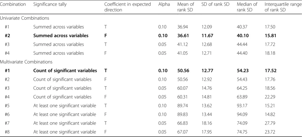
There were differences between the average standard devi-ation of ranks across trials for all 12 combindevi-ations (Table 1), and most pair-wise comparisons between combinations were significantly different (not shown). Univariate com-bination #2 had the lowest variability in the univariate group (mean standard deviation = 36.6 positions), while multivariate combination #1 had the lowest variability in the multivariate group (mean standard deviation = 50.6 po-sitions). These were chosen as the most promising combi-nations for further analyses, as described in the following section. Univariate combination #2 counted a repetition as significant at the 0.10 level without considering the direc-tion of the effect. Multivariate combinadirec-tion #1 counted the number of variables that were significant at the 0.10 level when the effect was in the expected direction (Table 1). Table 1Summary of variants for each combination and standard deviations (SD) for case ranks between trials
Combination Significance tally Coefficient in expected direction
Alpha Mean of rank SD
SD of rank SD Median of rank SD
Interquartile range of rank SD Univariate Combinations
#1 Summed across variables T 0.10 36.94 12.09 40.37 17.50
#2 Summed across variables F 0.10 36.61 11.67 40.10 15.81
#3 Summed across variables T 0.05 41.12 12.68 44.44 17.72
#4 Summed across variables F 0.05 41.05 12.71 44.40 18.18
Multivariate Combinations
#1 Count of significant variables T 0.10 50.56 12.77 54.23 17.52
#2 Count of significant variables F 0.10 50.56 12.92 54.43 17.76
#3 Count of significant variables T 0.05 60.07 14.76 64.25 18.56
#4 Count of significant variables F 0.05 60.31 14.81 63.89 22.29
#5 At least one significant variable T 0.10 89.74 13.62 93.17 15.21
#6 At least one significant variable F 0.10 89.83 13.44 94.09 14.82
#7 At least one significant variable T 0.05 66.83 18.16 74.09 27.79
#8 At least one significant variable F 0.05 67.07 17.95 74.75 23.72
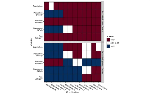
The statistical differences between the probable excess deaths and the pool of controls were assessed for each of the five variables (Fig. 2). The probable excess deaths identified by the univariate combinations were signifi-cantly different from the pool of controls with respect to all variables. Those identified by the multivariate combi-nations #1–4 (in which the number of significant vari-ables was tallied) were also significantly different from the controls for all variables, with the exception of greenness for combinations #3–4. Those identified by multivariate combinations #5–8 (in which the presence of at least one significant variable was tallied) did not differ from controls with respect to greenness or popula-tion density. Further, those identified by combinapopula-tion #7 (in which significance was tallied at the 0.05 level) did not differ from controls with respect to deprivation.
Statistical differences between the probable expected deaths and the pool of controls were also assessed for each of the five variables (Fig. 2), under the assumption that the differences would be small. The probable ex-pected deaths identified by the univariate combinations were significantly different from the pool of controls with respect to all variables except location of death,
though many of the p-values were in the 0.01 to 0.05 range. Those identified by the multivariate combinations #1–4 (in which the number of significant variables was tallied) were not different from the controls for the greenness and age category variables, and combinations #3–4 were not different for the location of death vari-able. Finally, those identified by multivariate combina-tions #5–8 (in which the presence of at least one significant variable was tallied) were only different from the controls for the location of death variable. Overall, it appears that differences were driven by one or two vari-ables for each group of combinations.
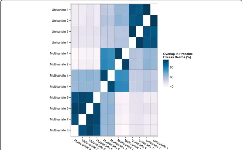
The percentage of overlap in the probable excess deaths identified between each pair of combinations was evaluated (Fig. 3). Univariate combinations #1–4 showed strong internal consistency with overlap of >90% be-tween all pairs. Multivariate combinations #1–4 showed similar internal consistency (mean overlap 81.9%), and so did multivariate combinations #5–8 (mean overlap 93.3%). The univariate combinations were more consist-ent with multivariate combinations #1–4 (mean overlap 58.0%), than with multivariate combinations #5–8 (mean overlap 45.6%). Multivariate combinations #3–4 were
also consistent with multivariate combinations #5–8 (mean overlap 62.9%). Overall, there were 30 decedents (26.3% of the total 114) who were identified as probable excess deaths by all 12 of the modelling combinations.
Further analyses on most promising combinations
Univariate combination #2 and multivariate combination #1 were selected for further analyses because they had the lowest variability in the standard deviations of rank (Table 1). Deaths from the pool of 411 cases were ran-domly selected into approximately 72% of the total five million repetitions (10,000 repetitions × 5 univariate models × 100 trials) for univariate combination #2, and one million repetitions (10,000 repetitions × 1 multivari-ate model × 100 trials) for multivarimultivari-ate combination #1. Deaths from the pool of 11,632 controls were selected an average of 10.2% of the time. In the univariate com-bination the mean ranks across 100 trials ranged from 3.9 to 410.3 (out of a possible 1.0 to 411.0) for the pool of cases, compared with 20.39 to 396.70 for the multi-variate combination. The standard deviations of the ranks ranged from 1.1 to 54.3 positions for the univari-ate combination, and from 13.5 to 75.3 positions for the multivariate combination. The greatest consistency in rank was found in the highest and lowest ranked cases.
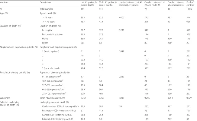
Distributions of the five variables were compared between the 114 probable excess deaths from the two selected approaches (Table 2). The deaths identified in the univariate approach were significantly younger, had a significantly lower residential greenness, and were sig-nificantly more deprived than those identified in the multivariate approach. No significant difference was found between approaches in the location of death or the population density. We also summarized the under-lying causes of death for the probable excess deaths, according to categories of the ICD-10 (Table 2). The deaths identified by the univariate combination were shifted away from cardiovascular and respiratory causes compared with the multivariate combination, but shifted toward deaths from cancer and external causes starting with X in the ICD-10. The 17 probable excess deaths at-tributed to external causes in the univariate group in-cluded one highly-publicized death due to excessive natural heat and 16 deaths due to accidental poisonings by pharmaceutical or illicit agents and intentional self-harm. All but one of these deaths occurred at home or in the community.
Variable Description Uni. #2 probable excess deaths
Multi. #1 probable excess deaths p
-value between uni. #2 and multi. #1 results
Overlap between uni. #2 and multi. #1
Overlap between all combinations
Pool of controls
N Total number 114 114 72 30 11632
Age (%) Age at death (%)
< 75 years 83.3 52.6 <0.001 79.2 96.7 37.4
> = 75 years 16.7 47.4 20.8 3.3 62.6
Location of death (%) Location of death (%)
In hospital 37.7 37.7 0.288 34.7 0 51.9
Residential institution 17.5 27.2 19.4 0 30.9
Home 36.0 28.9 37.5 80.0 14.5
Other 8.8 6.1 8.3 20.0 2.7
Neighborhood deprivation quintile (%) Neighborhood deprivation quintile (%)
1 (least deprived) 6.1 0 0.049 0 0 20.7
2 4.4 0 0 0 20.7
3 20.2 14.0 15.3 20.0 19.2
4 21.9 33.3 26.4 13.3 19.1
5 (most deprived) 47.4 52.6 58.3 66.7 20.2
Population density quintile (%) Population density quintile (%)
0–181 persons/km2 1.7 0 0.829 0 0 20.1
182–526 persons/km2 8.8 1.8 2.8 3.3 19.5
527–681 persons/km2 10.5 18.4 8.3 16.7 19.9
682–2356 persons/km2 28.9 30.7 33.3 20.0 19.8
2357–2573 persons/km2 50.0 49.1 55.6 60.0 20.7
Greenness Mean NDVI measurement 0.252 0.290 0.008 0.256 0.254 0.329
Selected underlying causes of death (%)
Underlying cause of death (%)
Cardiovascular (ICD-10 starting with I) 17.5 28.1 NA 22.2 36.7 27.1
Respiratory (ICD-10 starting with J) 6.1 11.4 8.3 6.7 10.0
Cancer (ICD-10 starting with C) 36.0 25.4 30.6 10.0 30.7
External (ICD-10 starting with X) 14.9 8.8 13.9 26.7 3.1
Identified cases from the univariate and multivariate combinations were compared with respect to the five variables used in the analyses, as well as with respect to selected underlying causes of death. The overlap cases identified in both combinations (N= 72) and by all combinations (N= 30) were compared with the pool of controls
al.
Environme
ntal
Health
(2016) 15:109
Page
7
of
(compared with 37% among controls), 46% died in the community (17% among controls), 58% lived in the most deprived neighborhoods (20% among controls), 56% lived in the most densely populated neighborhoods (20% among controls), and there was lower vegetative green-ness surrounding their residences. These differences were more pronounced when the probable excess deaths were restricted to the 30 identified by all 12 combinations (Table 2).
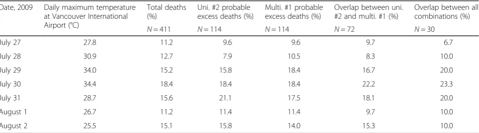
Finally, daily deaths during the extreme hot weather event ranged from 46 to 76, and all days were elevated above the summer 2009 mean of 42 (Fig. 1). Given that heat was assumed to be the underlying driver of in-creased mortality, we expected the probable excess deaths to be shifted towards the hotter days in the period. We assessed this by comparing the proportion of deaths on each day for: (1) all 411 deaths; (2) the 114 probable excess deaths identified by univariate combin-ation #2 and by multivariate combincombin-ation #1; (3) the 72 deaths identified by both combinations; and (4) the 30 deaths identified by all 12 combinations. The probable excess deaths were shifted towards the July 29–31 dates, and the shift was more pronounced among the 72 and 30 deaths that were identified by multiple model-ling combinations (Table 3). Even so, all approaches had some probable excess deaths occurring on every day of the event.
Discussion
Rapid epidemiologic assessment of mortality during extreme hot weather events is challenging because the excess deaths are almost always indistinguishable from the expected deaths in administrative vital statistics databases. Most excess deaths do not meet the criteria for certification due to excess heat [15], and are there-fore attributed to the same ICD codes as the expected deaths. However, statistical tools that facilitate rapid
epidemiologic assessment with these readily-available data could help generate timely evidence to protect vulnerable populations and to improve public health outreach during future events. The BCCDC has devel-oped the proposed methods to identify the most prob-able excess deaths during a 2009 hot weather event in greater Vancouver, Canada. The approach is predicated on the assumption that the expected deaths during a hot weather event are similar to deaths that occur during normal summer temperatures when compared with respect to variables known to be associated with hot weather mortality. The framework for the approach is a case-control analysis into which hot weather cases and typical weather controls were randomly sampled from larger pools. Over thousands of repetitions and 100 trials, probable excess deaths were identified as cases that were most consistently found in non-null models.
Several sensitivity analyses were conducted to explore the behavior of the framework across variations in the in-put parameters including model type, significance weight-ing, coefficient directionality, and significance level. The excess deaths identified and the standard deviations of their ranking across 100 trials were most sensitive to the model type, where univariate and multivariable combina-tions were tested. In comparison, the direction of the sig-nificant coefficients had little impact on the stability of the results, suggesting that the effects were in the expected direction in the majority of repetitions. Similarly, there was little difference between the 0.10 and 0.05 significance levels, but the combinations with the 0.10 level showed more internal consistency.
All of the univariate combinations were considerably more stable than the multivariate combinations when assessed by the variability of the rankings. However, neither approach was completely consistent with our a
priori assumption that the probable expected deaths would be similar to the pool of controls while the
Table 3Summary of deaths by day of the 2009 hot weather event
Date, 2009 Daily maximum temperature at Vancouver International Airport (°C)
Total deaths (%)
Uni. #2 probable excess deaths (%)
Multi. #1 probable excess deaths (%)
Overlap between uni. #2 and multi. #1 (%)
Overlap between all combinations (%)
N= 411 N= 114 N= 114 N= 72 N= 30
July 27 27.8 11.2 9.6 9.6 9.7 6.7
July 28 30.9 12.7 7.9 10.5 8.3 10.0
July 29 34.0 15.2 15.8 18.4 16.7 20.0
July 30 34.4 18.4 18.4 18.4 22.2 23.3
July 31 28.7 15.6 21.1 17.5 18.1 20.0
August 1 26.7 11.2 11.4 11.4 9.7 10.0
August 2 25.5 15.1 15.8 14.0 15.3 10.0
probable excess deaths would not (Fig. 2). There was also a marked lack of stability in the results from the multivariate combinations that counted a repetition as significant if any one of the five variables had a signifi-cant coefficient. This suggests that weighting the ranks for the number of significant variables in each repetition of the multivariable models produces more internal sta-bility. Given that the model type was the most important choice, it is possible that other modelling or machine learning approaches would produce more robust results.
Overall, the suite of analyses demonstrated that the specification of the modeling framework affects the set of cases that will be identified as probable excess deaths and any subsequent conclusions drawn from the methods. Furthermore, we have used the ecologic time-varying deprivation, greenness, and population density variables as if their respective 2006, 2009, and 2010 values were static across the region during the 2009– 2012 period. As such, both cases and controls may have been misclassified, which could bias the results if the actual exposures were systematically different from the estimates. For example, the City of Vancouver has planted many new street trees in recent years, meaning that the 2009 greenness estimates for the control popu-lation may be low when compared with the actual expo-sures. This could result in some cases with more moderate greenness values not being included in the group of probable excess deaths.
Another potential source of bias is the selection of the case and control periods. We defined the extreme event as July 27 through August 2 to be consistent with previ-ous work [17], but this period includes 2–3 days when mortality was within the normal range of variability (Fig. 1). The results would have been considerably differ-ent if we had limited the pool of cases to the dates with significantly elevated mortality. Likewise, the results might be different if we had restricted the pool of con-trols such that we were randomly sampling the same proportion from the case group (297/411) and the con-trol group (1,188/1,644) for each repetition. Ultimately, however, it would be ideal if we could test and refine this approach in a context where other, more conventional epidemiologic methods have been used to identify excess deaths. For example, Price et al. identified 106 of the 304 deaths as being heat-related via chart review after the 2010 event in Montreal [25]. Alternatively, the methods could be optimized using simulated data, in which the excess and expected deaths have been clearly defined. Ei-ther way, a dataset that included known excess deaths would allow refinement of the methods proposed here.
We have used deaths in the summers following the 2009 event as the pool of controls to simulate a conven-tional case-control study. However, the proposed methods could be most useful in the days and weeks following an
extreme event associated with an obvious increase in mor-tality. In such cases the pool of controls would be drawn from a period before the event, as was done for our prior case-only analyses with these data [17]. Indeed, the ideal public health response could comprise the following steps: (1) rapid case-only analysis to ascertain variables most strongly associated with death during the extreme event; (2) application of the proposed methods to identify the most probable excess deaths; (3) review of charts/death certificates to confirm the role of extreme hot weather; and (4) targeted case-control study using administrative data or other methods, depending on the resources. How-ever, the proposed approach is unlikely to be informative for short events with more subtle impacts, though it may be even more informative as the magnitude and/or duration of the exposure increases and its public health impacts are even further elevated above baseline.
The 30 cases identified by all 12 combinations were classified as the most probable excess deaths. These in-dividuals were significantly younger, more likely to die in the community, and they lived in more densely popu-lated, more deprived, and less green neighborhoods. Combined with the increase in external causes of death, which included deaths such as poisoning and self-harm, these results suggest that a marginalized population may be at highest risk in greater Vancouver. This is consistent with recent findings from the 2010 event in Montreal, where mental health illness was an important risk factor for death during the hot weather [25]. We cannot reliably evaluate the role of specific comorbidities or pharmaceuti-cals without access to death certificates or linkage between the vital statistics and other sources of administrative health data, but these results provide sufficient evidence to help target public health interventions during future episodes of extreme hot weather in the region.
Conclusion
Abbreviations
BC:British Columbia; BCCDC: British Columbia Centre for Disease Control; GWPv4: Gridded population of the world version 4; ICD: International classification of diseases; NDVI: Normalized difference vegetation index; VANDIX: Vancouver deprivation index; YVR: Vancouver International Airport
Acknowledgements
The authors would like to thank Ben Armstrong for reviewing the first draft of the manuscript and for providing suggestions about how to make the work stronger. This work was internally funded, though some salary support for JSG, SAR, KEM, and NK was provided by Health Canada. Finally, thanks to our reviewers whose insightful comments and suggestions helped us to refine the methods and the manuscript.
Funding
This study was funded as part of core activities at the BC Centre for Disease Control (BCCDC).
Availability of data and materials
The authors cannot make the raw data available to other researchers. However, we can make the analytic code available, along with a mock dataset to demonstrate the nature and structure of the data used.
Authors’contribution
SBH conceived of the study, designed and oversaw the coding and analyses, and led the draft manuscript. JSG led final development of the code, generated all data visualizations, and helped to draft the manuscript. SAR led initial development of the code and contributed to the study design. KEM led secondary development of the code, code testing, and helped to draft the manuscript. NK assisted with final development of the code, conducted all final analyses, and helped with preparation of the manuscript. DMH helped to conceive of the study design and helped to draft the manuscript. TK oversaw the entire project and helped to draft that manuscript. All authors read and approved the final manuscript.
Competing interests
The authors declare that they have no competing interests.
Consent for publication Not applicable.
Ethics approval and consent to participate
The British Columbia Centre for Disease Control (BCCDC) receives daily administrative vital statistics data for the purposes of public health surveillance and protection. Routine use of these data for such purposes is authorized under the provincial Public Health Act.
Author details
1Environmental Health Services, British Columbia Centre for Disease Control, 655 West 12th Avenue, Vancouver, BC V5Z 4R4, Canada.2School of Population and Public Health, The University of British Columbia, 2206 East Mall, 3rd Floor, Vancouver, BC V6T 1Z3, Canada.3Center for Policy Informatics, School of Public Affairs, Arizona State University, Phoenix, AZ 85004, USA.
Received: 18 September 2015 Accepted: 10 November 2016
References
1. Whitman S, Good G, Donoghue E, Benbow N, Shou W, Mou S. Mortality in Chicago attributed to the July 1995 heat wave. Am J Public Health. 1997; 87(9):1515–8.
2. Semenza JC, Rubin CH, Falter KH, Selanikio JD, Flanders WD, Howe HL, Wilhelm JL. Heat-Related Deaths during the July 1995 Heat Wave in Chicago. New England J Med. 1996;335(2):84–90.
3. Fouillet A, Rey G, Laurent F, Pavillon G, Bellec S, Guihenneuc-Jouyaux C, Clavel J, Jougla E, Hémon D. Excess mortality related to the August 2003 heat wave in France. Int Arch Occup Environ Health. 2006;80(1):16–24. 4. Vandentorren S, Suzan F, Medina S, Pascal M, Maulpoix A, Cohen J, Ledrans
M. Mortality in 13 French cities during the August 2003 heat wave. Am J Public Health. 2004;94(9):1518–20.
5. Conti S, Meli P, Minelli G, Solimini R, Toccaceli V, Vichi M, Beltrano C, Perini L. Epidemiologic study of mortality during the Summer 2003 heat wave in Italy. Environ Res. 2005;98(3):390–9.
6. Grize L, Huss A, Thommen O, Schindler C, Braun-Fahrlander C. Heat wave 2003 and mortality in Switzerland. Swiss Med Wkly. 2005;135(13-14):200–5. 7. Johnson H, Kovats S, McGregor G, Stedman J, Gibbs M, Walton H. The
impact of the 2003 heat wave on daily mortality in England and Wales and the use of rapid weekly mortality estimates. Euro Surveill. 2003;10(7):558. 8. Revich BA. Heat wave, air quality and mortality in European Russia in summer
2010: preliminary assessment. Yekologiya Cheloveka/Human Ecology. 2011;7:3–9. 9. Bustinza R, Lebel G, Gosselin P, Bélanger D, Chebana F. Health impacts of
the July 2010 heat wave in Québec, Canada. BMC Public Health. 2013; 13(56):1–7.
10. Lan L, Cui G, Yang C, Wang J, Sui C, Xu G, Zhou D, Cheng Y, Guo Y, Li T. Increased Mortality During the 2010 Heat Wave in Harbin, China. Ecohealth. 2012;9(3):310–4.
11. Sartor F, Snacken R, Demuth C, Walckiers D. Temperature, ambient ozone levels, and mortality during summer 1994, in Belgium. Environ Res. 1995; 70(2):105–13.
12. Tan J, Zheng Y, Song G, Kalkstein L, Kalkstein A, Tang X. Heat wave impacts on mortality in Shanghai, 1998 and 2003. Int J Biometeorol. 2007;51(3):193–200. 13. Ostro BD, Roth LA, Green RS, Basu R. Estimating the mortality effect of the
July 2006 California heat wave. Environ Res. 2009;109(5):614–9.
14. Tong S, Ren C, Becker N. Excess deaths during the 2004 heatwave in Brisbane, Australia. Int J Biometeorol. 2010;54(4):393–400.
15. Donoghue ER, Graham MA, Jentzen JM, Lifschultz BD, Luke JL, Mirchandani HG. Criteria for the diagnosis of heat-related deaths: National Association of Medical Examiners: position paper. Am J Forensic Med Pathol. 1997;18(1):11–4. 16. Kovats S. Heatwave of August 2003 in Europe: provisional estimates of the
impact on mortality. Euro Surveill. 2004;8(11):2409.
17. Kosatsky T, Henderson SB, Pollock SL. Shifts in Mortality During a Hot Weather Event in Vancouver, British Columbia: Rapid Assessment With Case-Only Analysis. Am J Public Health. 2012;102(12):2367–71.
18. Mirchandani HG, McDonald G, Hood IC, Fonseca C. Heat-related deaths in Philadelphia-1993. Am J Forensic Med Pathol. 1996;17(2):106–8. 19. Shen T, Howe HL, Alo C, Moolenaar RL. Toward a Broader definition of
heat-related death: comparison of mortality estimates from medical examiners’ classification with those from total death differentials during the July 1995 heat wave in Chicago, Illinois. Am J Forensic Med Pathol. 1998;19(2):113–118. 20. Henderson SB, Kosatsky T. A Data-driven Approach to Setting Trigger
Temperatures for Heat Health Emergencies. Can J Public Health. 2012; 103(3):227–30.
21. Doxsey-Whitfield E, MacManus K, Adamo SB, Pistolesi L, Squires J, Borkovska O, Baptista SR. Taking Advantage of the Improved Availability of Census Data: A First Look at the Gridded Population of the World, Version 4. Papers in Applied Geography. 2015;1(3):1–9.
22. Bell N, Schuurman N, Oliver L, Hayes MV. Towards the construction of place-specific measures of deprivation: a case study from the Vancouver metropolitan area. Canadian Geographer/Le Géographe canadien. 2007;51(4):444–61. 23. Pettorelli N, Vik JO, Mysterud A, Gaillard JM, Tucker CJ, Stenseth NC.
Using the satellite-derived NDVI to assess ecological responses to environmental change. Trends Ecol Evol. 2005;20(9):503–510. 24. Yuan F, Bauer ME. Comparison of impervious surface area and normalized
difference vegetation index as indicators of surface urban heat island effects in Landsat imagery. Remote Sens Environ. 2007;106(3):375–86.