Cost Function Modelling for Semi-automated SC, RTG and Automated and Semi-automated RMG Container Yard Operating Systems
Mansoor Kiani Moghadam∗ Roya Noori∗∗
Abstract
This study analyses the concept of cost functions for semi-automated Straddle Carrier (SC), Rubber Tyred Gantry (RTG) and automated Rail Mounted Gantry (RMG) container yard operating cranes. It develops a generic cost based model for a pair-wise comparison, analysis and evaluation of economic efficiency and effectiveness of container yard equipment to be used for decision-making by terminal planners and designers. The cost function analysis of this study incorporates major cost attributes used in modern container terminal operations and discussed in the literature. They play a determining role over the total cost of advanced operating systems in a container terminal. The cost model in this study enables the planner and designer of container terminals to make a pair-wise comparison of handling systems to help determine the most appropriate container yard operating system for a port, based on the required technological capabilities and functions. The sensitivity analysis proposed in this study compares and demonstrates the magnitude and intensity of the selected attributes which determine preference of one system over another. The analysis assists a terminal planner in decision-making and selecting a container yard operating system with a minimum operating cost and a maximum annual throughput.
Keywords: Container terminal, Cost Function Modelling, Sensitivity Analysis.
1. Introduction
The operation of advanced technologies including automated and semi-automated equipment in container terminals has reduced the time
∗
of transferring, stacking and retrieving of containers in marshalling yards. The adoption of automated devices has increased the efficiency of the shipside, quayside, marshalling yard, gate and transfer operations. This in turn has reduced the loading and discharging time, dwell-time, cycle-time of container and transfer vehicle movements and consequently the total turnaround-time of containerships in ports. A variety of advanced systems such as semi-automated Straddle Carriers (SCs) capable of transferring and stacking containers to a height of 1 over 3 or more, Automated Guided Vehicles (AGVs) and shuttles capable of automatically transferring containers without human intervention have been involved in the operation of container terminals during the last two decades. At the stack-yard, semi-automated Rubber Tyred Gantry cranes (RTGs) and fully automated Rail Mounted Gantry cranes (RMGs) have been deployed for operation in today’s modern container terminals.
Medecentre Tauro in Italy and Hutchinson Freeport in Bahamas with a high capacity which are considered as the container terminals with a high transhipment ratio have successfully employed SC as their main transfer and stacking system (Avery, 1999). The SC system is preferred over other systems in many container terminals due to its versatility and relatively low purchasing cost per unit of equipment, smaller marshalling yard development and operation costs. However, there are some drawbacks with SC operating systems. The SC systems utilise less space in terms of m2 / TEU, lower stacking ability, require more area
for receipt and delivery operations, require higher maintenance and greater down-times and are less suitable for automation. On the other hand, yard gantry cranes such as RTG and RMG cranes are more space efficient, more accurate and faster in operation and are more suitable for development and instalment of automated technologies (Watanabe, 2001). The yard gantry cranes however require a higher development and land preparation costs than SC systems due to their high wheel load and body weight. RTGs are more flexible and more economic to purchase and install, but more expensive to operate than RMGs (Containerisation International, 1996).
2. Literature review
2002) have developed a cost model for different space layouts and transfer systems and included different cost variables in their analysis. They have suggested a cost model which incorporates the fixed investment and variable operations costs to be used to help decision-making. Two objectives have been suggested to be met in their analysis. These objectives are the minimisation of the total cost of terminal operations and the costs associated with customers using a terminal. Zhow et al. (2001) have proposed a cost comparison model for various container stacking and handling systems. Their model provides comprehensive methods to calculate the maximum throughput and the optimum total cost of the operating system and revenues derived from the operations in container terminals.
different studies carried out by Yang et al. (2004) and Vis and Harika (2004), the optimum productivity of automated container terminals with minimum possible costs has been discussed. It has been argued that ALVs including automated SCs provide higher productivity and cost effectiveness principally because they can eliminate the waiting-times of the transfer vehicles at the stack-yard. In different studies conducted by Kiani et al (2006-a, 2006-b, 2009) the economic feasibility of automated quayside cranes has been evaluated and in the later research a break-even model has been formulated to evaluate the cost of containerships’ waiting-times and berth unproductive-times in automated quayside operations. Kiani et al (2009) have also developed a concrete decision tool to show the viability and applicability of multiple attribute decision-making (MADM) and analytical hierarchy process (AHP) methods in the selection decisions for a container yard operating system.
3. Analysis of cost parameters and variables
beyond the scope of this study. The parameters and variables may be categorised and defined into three groups as follows:
3.1 Container yard development and maintenance costs
For different ports situated in different geographical and political locations, there are different factors that may affect the volume of investment and consequently the development and maintenance of the purchased or leased land. These factors may range from subsidies, loans and borrowings to the physical features of a container terminal site such as costs involved in civil engineering, hydrography, topography, meteorological and oceanography influences, coastal hydraulics and environmental issues (UNCTAD, 1985). However, factors and issues such as those mentioned above are considered beyond the scope of this study. In this study, four major factors related to the land investment, development, maintenance and depreciations are considered. For almost all of the Iranian ports such as the BACT, BICT and CCT, the land within the port area has been retained as the property of government. Therefore, the initial cost of investment in land in the examples of the Iranian ports may differ significantly from European countries and many Asian countries such as Japan, Singapore and Hong Kong. This study includes the following factors in the proposed cost model:
Cost of investment in land
The Port and Shipping Organisation of Iran (PSO) have leased out some part of the land in its port environment to private sectors operating the terminals. The values are approximate and are contracted for about 40 to 50 years. These values are stated in Table (1).
Table (1) Average annual cost of investment in land
Cost of Investment in Land £ / m2 / Year
Port
1990-1994 1995-1999 2000-2004
BACT 23.60 25.00 27.20
BICT 19.50 28.40 31.30
Container yard development cost
The cost of container yard development may vary from terminal to terminal due to the variations in the site construction and conditions. One may devote a considerable budget for preparation of the container yard surface, turning areas, road and passageway accesses, ducting and cable laying preparations, drainage, light stands, etc. It should be noted that the surface of the container yard and its receipt and delivery areas, turning areas and the junctions of the road and passageways must be prepared to withstand loads of about 80-120 tonnes (Nahavandi, 1996). The terminal operator in BACT has considered a cost of £20 to £23 / m2
in land preparation in 2004 for SCs operating system. In mid-2003 in BICT, an average of £52 / m2 was spent on the preparation of stacking
areas for the new modern 12+2 RMG system (Zahiri, 2005). This study considers a cost of £23 to £52 / m2 which is used for the preparation of
the container yard for CCT.
Container yard development depreciation cost
The facilities used in the development of a container yard stated in the previous section will wear out over time. This may require the operator of container terminals to consider an annual depreciation cost for development of facilities in their calculations. This study uses the depreciation method recommended by UNCTAD and proposed by Constantinides (1990). Generally the annual depreciation of a system is obtained by subtracting the salvage value of the equipment from the initial cost of investment and dividing the results by the expected project life of the system. In this study a salvage value proportional to about 20% of the initial cost of investment in the container yard development is considered.
Container yard maintenance cost
2004). In this study, a fraction of 0.15% of the initial cost of investment is considered for the analysis.
It should be noted that in calculating the maintenance costs of a system, one should consider the wear and tear of the assets (particularly equipment) which would increase over time. As the economic life of the container yard and equipment increases the annual maintenance cost increases at an exponential rate (Guthrie and Lemon, 2004). This implies that the annual maintenance cost of a system is minimum in year one and would be maximum at the end of its project life. For the purpose of this study, the Future Worth Factor (FWF) method recommended by UNCTAD (Constantinides, 1990), Nahavandi (1996), UNCTAD (2002) and Guthrie and Lemon (2004) will be used for calculation of the annual maintenance costs for container yard development and yard cranes.
3.2. Crane investment, manning and maintenance costs
The costs and attributed factors related to the investment, operation and maintenance of a container yard operating system might be categorised as follows:
Crane procurement cost
The purchasing price of container yard operating systems depends on factors such as:
i) Order time. ii)Order size.
iii)Place and location of manufacturer from the purchaser.
iv)Equipment specification (type, capacity, size, degree of automation, crane lateral speed, number, type and speed of trolley and hoist, etc.). v)Variations in market prices.
Table (2) Average procurement cost of container yard operating systems, £/equipment
RTG RMG SC
5 +1 6+1 11+2 12+2
Year
1 over 2 1 over 3 1 over 4 1 over 4 1 over 5 1 over 4 1 over 5 1 over 4 1 over 5 1 over 4 1 over 5 1990-1994 175,300 190,550 - 217,250 228,570 230,350 247,500 522,320 566,320 587,140 604,450 1995-1999 191,750 212,310 - 321,200 330,240 385,870 407,760 612,550 633,540 609,240 614,250 2000-2004 232,450 260,870 290,780 394,200 419,150 440,400 471,550 640,100 667,140 610,320 623,200
(Source: Compiled by author)
Annual cost of capital investment in cranes
The cost of capital investment in any container yard operating system may depend on the number, procurement cost, average economic life of cranes and the average interest rate expected during such a period.
Economic life of cranes (t)
The theoretical economic life of container yard equipment is usually given by the manufacturer as the number of full cycles, movements and/or travels performed by the equipment. In practice, these values may differ from terminal to terminal under different operational and climatic conditions. The actual economic life of the equipment may, however, depend on the extent of utilisation, maintenance efficiency, skill of operators and the magnitude of hazards affecting the equipment. UNCTAD, (1990), Containerisation International, (1996) and some terminal operators have proposed different values of economic life. The average economic life of container yard operating systems has been compiled from different sources and tabulated in Table (3). The practical economic life of equipment for BACT may be considered shorter than the theoretical values recommended by UNCTAD. This is due to the fact that most Iranian ports are located in a tropical climate and are more vulnerable to corrosion, wear and tear in a temperate climate.
Table (3) Average economic life of QSCs, SC, RTG and RMG cranes, years
Recommending Body QSCs SC RTG RMG
UNCTAD 10-12 6-10 15-18 -
Containerisation International 10-14 15-20 15-20 20-22
Manufacturers 12-15 10-16 12-16 18-22
Port Operators 12-15 10-15 12-15 15-20
Crane depreciation cost
The depreciation of yard cranes may be considered as a process by which a container terminal gradually loses the fixed value of its investment in the equipment. The purpose of including crane depreciation cost is to spread the initial purchase price of the equipment over its useful life. It may be defined as the difference between the initial cost of investment and the salvage value of the equipment expressed as present values divided by its economic life. UNCTAD (1985) and Constantinides (1990) have proposed a fraction of about 20% of the initial cost of investment as a salvage value for SC, RTG and RMG systems after their economic lives are over. In this study the fraction recommended by UNCTAD will be considered for yard cranes.
Crane maintenance costs
The maintenance cost of SC, RTG and RMG systems is considered in this study. The maintenance cost varies from equipment to equipment depending on the mobility, speed, type of fuel, number of moves etc. The annual maintenance cost of yard cranes is normally taken as a percentage of the initial cost of investment over the economic life of the cranes. UNCTAD (1985) and Constantinides (1990) have proposed 1.0% to 1.2% and 1.8% of capital cost of investment for a SC system respectively. Their proposed percentage includes the cost of fuel, consumables such as lubricating oil, tyres, spare parts, etc. Watanabe (1995) has proposed 1.5% of initial investment and has included cost of fuel and spare parts too.
(1985) and Constantinides (1990) have suggested that about 1.0% of the initial cost of investment to be considered for RTG and RMG systems. In BACT, the maintenance cost of a SC system is about 0.8% whereas, in BICT the value for electrical power driven RMGs is between 0.3% to 0.4% and diesel RMGs is between 0.5% to 0.6% of the initial cost of investment (Bahrani, 2004). Wear and tear of the road and passageways for RTGs particularly at the junctions and turning areas may be more than that of a SC system therefore, it may be reasonable to consider a higher percentage for the cost of maintenance for an RTG system. It should be noted that some terminals having four wheel RTGs have concrete beams to reduce wear and tear (Watanabe, 2001). This study uses the method proposed by UNCTAD (Constantinides, 1990) and Nahavandi (1996) for calculation of the equipment annual maintenance cost.
Inter-yard operation cost of cranes
An attribute that may be used as a performance indicator between different systems is the average Cost Per Container (CPC) movement in a terminal. This value would be dependent on the annual throughput of a terminal. The annual capacity for container terminals with different sizes operating under SC, RTG and RMG systems with different container dwell-times, transhipment ratio and stacking height has been calculated in different studies during this research and will be used in this study. The average value for the direct SC system in BACT is about £0.4/move. The value for the electrically driven RMGs in BICT is about £0.2/move and £0.3 / move for the diesel driven equipment (Bahrani, 2004). Conservatively, one may consider about £0.6 /move for an RTG system.
of a competent crane driver and a container yard foreman including insurance, training, bonuses, incentives, etc. is about £13,440 / year (£1,120 / month) to £16,500 / year (£1,375 / month) (Bahrani, 2004).
3.3 Container transfer cost
The average annual cost of container transfer to and from the quayside to the stack-yard may be expressed as an average cost of handling operation fulfilled by AGVs in RMG or RTG systems, SCs in a SC direct system, internal trucks or T-Ts in the SC relay system or other means of transferring and marshalling containers between the quayside and the stacking area. The calculated average cost may include the cost of fuel, maintenance, insurance, etc. In both BACT and BICT, the transfer operation has been contracted out to the private sector. A fixed cost has been agreed to be paid to the private operator according to the number of containers handled. A total amount of about £0.10, £0.20 and £0.25/container/move may be considered for SC, RTG and RMG systems respectively (Bahrani, 2004).
4. Cost function modelling
One of the most difficult decisions at the planning stage of the container terminals is to make a decision on the most suitable container yard operating system for a terminal. Decisions should be made strategically for a long-term run of terminals. It is also difficult to indicate as to where and to what point in the time the terminal is going to stand in the future. Is the terminal going to develop the present Origin-Destination (O-D) stage into a Hub-Port (HP) status at some time in the future? Is it likely that land becomes less expensive and more available for future expansion of the terminal? What would be the cost of the development of a specific operating system in the terminal? There would be many questions that should be clearly answered before the final decision is made.
There are other cost related attributes, some of which are qualitatively expressed, that play a determining role and affect the layout, design and final selection decision of container yard equipment in a terminal. They can be categorised as follows:
Calculated annual throughput.
Under portal span and vertical lifting capacity of the container yard equipment.
Type, number and level of technology of container yard equipment. Ease of maintenance and repair.
Strength of the container yard construction. Economic life of the equipment.
Environmental and social considerations.
This study only considers SC, RTG and RMG systems. The cost model developed in this study comprises the following elements:
1)Land cost and container yard development and maintenance cost. 2)Cost of equipment, maintenance and manning for a specific container
yard operating system. 3)Transfer cost.
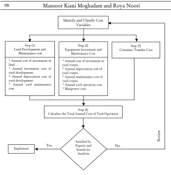
There will be more cost elements such as administration costs, cost of inflation, possible rise in the price of land, fuel consumption, and spare parts etc., which are out of the scope of this study. It should be noted that different container yard operation systems require different facility, preparation and installation and training costs etc. These may affect the total annual cost of the system. A trade-off can be made between the cost of the land and equipment and operation costs for the container yard system to be employed. This study develops a cost based method with the steps indicated in Figure (1) and the process as follows:
Figure (1) Cost function process
(Source: Author)
Step (1) Land development and maintenance costs
Steiner (1992), Thuesen and Fabrycky (1993), UNCTAD (2002) and Guthrie and Lemon (2004) have proposed applying a Capital Recovery Factor (CRF) to calculate the annual cost of investment for `t` years of a project life [see Appendix (1)]. The cost of land for a container yard operating under a specific operating system can be defined in the following process:
Identify and Classify Cost Variables
Implement Step (1) Land Development and
Maintenance cost
* Annual cost of investment in land.
* Annual investment cost of yard development.
* Annual depreciation cost of yard development
* Annual yard maintenance cost.
Step (2) Equipment Investment and
Maintenance Cost
* Annual cost of investment in yard cranes.
* Annual depreciation cost of yard cranes.
* Annual maintenance cost of yard cranes.
* Annual yard operation cost. * Manpower cost.
Step (3) Container Transfer Cost
Step (4)
Calculate the Total Annual Cost of Yard Operation
Satisfied by Experts and Sensitivity
Analysis
Yes No
Re
vi
Annual cost of capital investment in land
LC = CL x AT x CRF (1)
where:
LC = Annual cost of investment in land in £ / year. CL = Average cost of one square metre of land in £ / m2.
AT = Total area of container terminal for a specific container yard operating system (including stack-yard + gate, CFS, workshop area, rail and transhipment buffers + Interchange area, if appropriate, roadways, etc.) in m2.
CRF = Capital recovery factor which converts the initial investment into an equivalent average annual cost of equal series calculated as follows:
1 -i) + (1
i) + (1 × i =
CRF t
t
(2)
t = Economic life of the terminal in years. i = Average annual interest rate.
Annual container yard development cost
YDC = CD x AT x CRF (3)
where:
YDC = Annual container yard development cost in £ / year.
CD = Development cost of one square metre of land for a specific container yard operating system in £ / m2.
Annual depreciation cost of container yard development
t S -AT) × (CD = C
Ydep yard (4)
where:
YdepC = Annual depreciation cost of container yard development in £ /
year.
Syard = Salvage value of facilities in £.
Annual container yard maintenance cost
This study uses the FWF method recommended by UNCTAD (Constantinides, 1990) and UNCTAD (2002) [see Appendix (1)] as follows:
YMC = CYM x FWF (5)
YMC = Annual cost of container yard maintenance in £ / year.
CYM = Average annual maintenance cost of a specific container yard operating system in £.
FWF = (1+i)t-1
where:
t = Economic life of the terminal in years. i = Average annual interest rate.
Step (2) Crane investment, manning and maintenance costs
This study assumes that only one type of operating system such as SC, RTG or RMG would be operating in the terminal. Although a combination of the above systems with other modes of operation is possible, the analysis of their effect is not considered in this study. The costs involved in any specific operating system may be defined in the following process:
Annual cost of investment in yard cranes
IC = PC x NC x CRF (6)
where:
IC = Annual cost of capital investment in container yard operating system in £ / year.
PC= Procurement cost of a yard crane in £.
NC = Average number of RMGs, RTGs or SCs (adopted from previous studies conducted by authors).
Annual depreciation cost of yard cranes
t S -PC =
DC crane (7)
where:
DC = Annual depreciation cost of yard cranes in £ / year.
Scrane = Salvage value of a specific container yard operating system.
t = Average economic life of the cranes in years. Annual maintenance cost of yard cranes
(Constantinides, 1990), Nahavandi (1996) and UNCTAD (2002). This can be formulated as:
MCC = PC x FWF (8)
where:
MCC = Annual maintenance cost of a container yard operating system in £ / year.
PC = Average annual maintenance cost of equipment in £. FWF = (1+i)t-1
where:
t = Average economic life of the cranes in years. i = Average annual interest rate.
In-yard operation cost
OC = HCTEU x CY x CRF (9)
where:
OC = Annual cost of in-yard-handling operation of containers in £ / year.
HCTEU = Cost of handling of one container in £ / container (An average
cost for one TEU and / or 2 x TEU may be taken).
CY = Annual throughput of a terminal in TEUs (adopted from previous
studies conducted by the authors). Manning cost
Two types of workers are normally involved in the daily operation of a container yard. They are the yard gantry drivers and foremen who coordinate the operation of container transfer from the quayside to container stack-yard and vice versa. Where the container yard operation is fully automated, then there would not be such a work force. Instead, a few automation technicians would be available at all times to support yard cranes. The average salary of technicians is expected to be high in today’s container terminals. In this contest, the cost of crane operator and container yard foremen therefore can be defined as:
i) Crane operators cost
CD shift driver
shift
driver=NL ×N ×AS
LC (10)
LCdriver = Annual cost of work force for all cranes (including
stack-yards, gate, rail and transhipment buffers, empty and refer stacks, etc.) in £ / year.
driver shift
L
N = Number of crane divers in each shift. Nshift = Number of shifts in 24 hours.
ASCD = Average annual salary of a crane driver including taxes,
insurance, incentives, etc. in £ / year / person. ii) Coordinating foremen cost
LCYFM = NYFday x Nshift x ASYF (11)
where:
LCYFM = Annual cost of all container yard foremen in £ / year.
NYFday = Number of container yard foremen for the coordination of
the QSCs and yard cranes in each day.
ASYF = Average annual salary of a container yard foreman including
taxes and all other benefits in £ / year / person.
Step (3) Container transfer cost
Depending on the type of container yard system employed in a terminal, the transfer of containers between the quayside and the container yard, and vice versa, may be carried out by a SCs, T-Ts, AGVs, etc. The cost of container transfer by SC relay system and other modes of transfer such as AGV, lift trucks, T-Ts etc., may be higher than a SC direct system. The total cost of container transfer excluding the costs of transfer equipment such as maintenance, depreciation and cost of investment can be defined as:
Ctransfer = CTEU x CY x Nmoves (12)
where:
Ctransfer = Annual cost of container transfer operation in £ / year.
CTEU = Average cost of handling one container in £ / container.
CY = Annual throughput of the corresponding container terminal in
TEUs.
Nmoves = Average number of moves per container performed by a
Step (4) Total container yard operation cost
The Total Cost (TC) of a container yard operating system will be the summation of all costs involved in Steps (1) to (3). The equation can therefore be defined as follows:
TC=LC+YDC+YdepC+YMC+IC+DC+MCC+OC+LCdriver+LCYFM
+Ctransfer (13)
This study introduces the concept of a `cost comparison indicator` that will help a port designer to measure the percentage of cost effectiveness of one container yard operating system over another.
5. Sensitivity analysis
To help the terminal operator in making decisions, this study introduces the concept of a cost comparison process for the sensitivity analysis. The `cost comparison indicator` analyses the cost effectiveness of one-container yard operating system over another in terms of investment, maintenance, operation, depreciation, etc. The `Variable Intensity Factor` (VIF) method analyses the cost effectiveness of the selected parameters by demonstrating the magnitudes of the parameters with each other.
5.1 Cost comparison indicator
The selection of a cost effective operating system may be done by comparison of similar cost parameters, for example, the annual costs obtained for each container yard operating system (TCY) in Step (4). Where the annual cost of a system is considered as a criterion, a semi-automated SC operating system may be preferred over a semi-semi-automated RTG or an automated RMG system from a cost effective standpoint when TCYSC<TCYRTG and TCYSC<TCYRMG. A semi-automated RTG
system may be preferred over a SC or an automated RMG system when TCYRTG<TCYSC and TCYRTG<TCYRMG. This study denotes variables
k j j/k TCY TCY =
R (14)
m j j/m TCY TCY =
R (15)
k m m/k TCY TCY =
R (16)
Other combinations are possible. In this process and under the lowest-cost-preference policy, for example, if Rj/k < 1 the `j` container yard
operating system is preferred over `k` system. There would be of course no preference of a system over another if Rk/j =1. Therefore, a
sensitivity analysis would be required to indicate each case comparison by indicating the value of Rj/k = 1 as a benchmark to help better indicate
such a relation.
5.2 Variable Intensity Factor (VIF)
The variables and parameters identified in the development of the cost model may vary significantly from each other, from port to port and from time to time. Therefore, a further sensitivity analysis is required to represent the magnitude of a preference of a container yard operating system over another by taking the individual cost parameter in the analysis. A terminal designer and or a port operator may vary the value of any of the cost parameters and keep others unchanged to observe the impact of cost changes under the new condition. The operator may consider one or more particular cost parameters as the important and / or governing cost factors to be analysed. For example, a terminal planner may be interested in purchasing a SC rather than a automated RTG system or switching from a SC to a semi-automated RTG system. Therefore, the operator can calculate the magnitude of his / her preference of SC over RTG using specific cost parameters, cost intensity factor (R) and Variable Intensity Factor (VIF).
Hee and Wijbrands (1988) have defined the VIF as:
j k k / j j k / j CP CP R CP VIF − ×
= (17)
where:
VIFj/k = Variable intensity factor of `j` operating system over `k`
CPk = Value of cost parameter `k`.
CPj = Value of cost parameter `j`.
CPk≠ CPj
The value of `VIF` will indicate the relative degree of preference of one system over another. The higher the positive value becomes the higher the desire to employ a system will be. When the value of `VIF` of a system, for example `j` system over `k` system, becomes negative, that is to say VIFj/k < 0, it may indicate that `j` system is no longer
desirable over `k` system. This undesirability of course will be based on the specific cost component considered in the analysis. Depending on the magnitude and the sign of the value (being of a positive or a negative value) calculated for different combinations of cost factors, it may be argued that `j` system may or may not be considered preferable over `k` system. When the value of VIFj/k becomes negative, it is valid to
assume that the `k` system possesses more preferability over `j`. In this case the value of VIFk/j may not be equal to the VIFj/k value even with a
different sign and polarity. This means that the exact value of VIFk/j
requires to be calculated in the same way. It should be noted that when the values of CPk and CPj are close to each other, then the VIF result
produced may be very high and therefore unreliable. To avoid uncertainties in calculating the value of VIF, it would be better to select cost factors with unequal values and preferably with a high difference between the values of the pairs.
6. Test case
The Port and Shipping Organisation of Iran that owns most of the active ports in Iran is transforming the former Kalantry Port in Chabahar into a modern automated container terminal to facilitate the transfer of containers through land modes of transport to Europe via
converted to Pounds Sterling equivalent for the purpose of this study. The following assumptions are made:
a)Size of the container yard is assumed to be 350m x 400m (14 hectares) similar to the BACT.
b)Average interest rate of about 8% to be considered.
c)An estimated cost of £38 / m2 for a long-time rent (usually 50 years
for Iranian ports and renewable) for land investment has been assumed.
d)Cost of development of about £23, £38 and £52 / m2 for SC, RTG and
RMG systems has been considered respectively.
e)Container yard maintenance cost of about £7,980 [0.15% x £38 x 350m x 400m (14 hectares)] for SC, RTG and RMG systems to be considered.
f) The economic life (t) of container terminal is about 50 years.
g)Procurement cost of SC (1 over 3) = £260,870 / equipment, RTG 6+1 (1 over 5) = £471,550 / crane and RMG 12+2 (1 over 5) = £623,200 / crane.
h)Number of yard cranes taken from previous studies by the authors is about 63 for SC, 30 (2 RTG x 15 blocks) for RTG and 24 RMG (2 RMG x 12 blocks) for RMG systems (Kiani, 2007).
i)Average economic life (t) of a SC = 15 years, RTG = 15 years and RMG = 20 years.
j)This study considers about 20% of the initial investment cost of container yard development and 10%, 20% and 30% of the initial investment cost of SC, RTG and RMG cranes as salvage values in Iran after their economic life is over.
k) An average of 1.0%, 0.8% and 0.4% of the initial procurement cost of SC, RTG and RMG would be considered for the annual maintenance cost of the cranes respectively. Therefore, the average annual maintenance cost of yard cranes would be as follows:
SC = £260,870 x 63 x 1.0% ≈ £164,348 RTG = £471,550 x 30 x 0.8% = £113,172 RMG = £623,200 x 24 x 0.4% ≈ £59,827
m)Maximum annual throughput of SC (1 over 3) = 1,379,876 TEUs / year, RTG 6+1 (1 over 5) = 1,972,196 TEUs / year and RMG 12 +2 (1 over 5) = 2,113,168 TEUs / year (obtained from previous studies conducted by the authors).
n)Average salary of a competent driver and a container yard foreman is considered about £15,000 and £17,500 / year respectively. There would be 3 shifts a day where the terminal is considered to be operating 24 hours / day and 365 days a year.
o)Number of crane drivers in each shift is assumed to be 40 persons for SC, 20 persons for RTG and 15 persons for RMG systems.
p)Number of container yard foremen for SC = 4, RTG = 3 and RMG = 2 persons.
q)Transfer costs of about of £0.10, £0.20 and £0.25 / container are considered for SC, RTG and RMG systems respectively. Transfer vehicles are considered to perform at least two continuous moves in each job assignment.
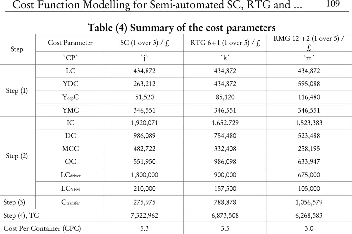
Table (4) Summary of the cost parameters
Cost Parameter SC (1 over 3) / £ RTG 6+1 (1 over 5) / £ RMG 12 +2 (1 over 5) / £ Step
`CP` `j` `k` `m`
LC 434,872 434,872 434,872 YDC 263,212 434,872 595,088
YdepC 51,520 85,120 116,480
Step (1)
YMC 346,551 346,551 346,551 IC 1,920,071 1,652,729 1,523,383 DC 986,089 754,480 523,488 MCC 482,722 332,408 258,195
OC 551,950 986,098 633,947
LCdriver 1,800,000 900,000 675,000
Step (2)
LCYFM 210,000 157,500 105,000
Step (3) Ctransfer 275,975 788,878 1,056,579
Step (4), TC 7,322,962 6,873,508 6,268,583 Cost Per Container (CPC) 5.3 3.5 3.0
6.1 Cost comparison and sensitivity analysis using `R` values
The values of cost comparison indicator (R) for different parameters are calculated and summarised in the second, third and fourth columns in Table 6.6 (second, third and fourth columns). The attributed cost factors indicated in the table show that from a minimum cost policy standpoint, a SC system may be preferred over a semi-automated RTG system where it produces a lower value of `R` (R<1) for cost factors such as `Ctransfer`, `OC`,`YdepC` and `YDC`. In cases where the value
of `R= 1`, then there would be no preference of one system over another. For R>1 values such as `LCdriver`, `CPC`, `MCC`, `TC`,
`DC` and `IC`, a SC system is no longer preferred over an RTG system. A SC may be preferred over an automated RMG system only where the cost parameters such as `Ctransfer`, `YDC`, `OC` and `YdepC`
have produced a lower `R` value than `1`. However, the comparison indicator implies that for the rest of cost parameters such as `LCdriver`,
`CPC`, `LCYFM`, `TC`, `MCC`, `DC`, and `IC` and except `LC`
1. 000 0. 605 0. 605 1.
000 1.162
1.
307 1.452
0. 560 2. 00 0 1. 333 0. 35 0 1. 065 1. 523 0.000 0.250 0.500 0.750 1.000 1.250 1.500 1.750 2.000 2.250 Cost Parameters
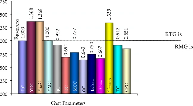
parameters except `Ctransfer`, `YDC` and `YdepC`, the other parameters
promise a lower cost ratio to prefer an automated RMG to a semi-automated RTG system. There is no preference of one system over another in `LC` and `YMC` cost parameters.
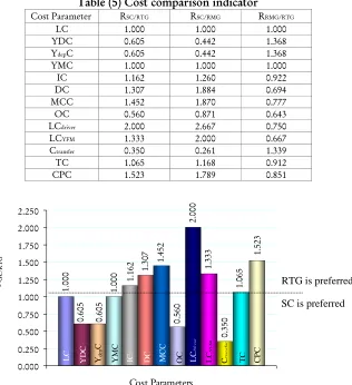
For an easier concept, the results of the three columns are illustrated in Figures (2), (3) and (4). The horizontal line drawn at `R = 1` indicates an indifference level above / below which other systems may be preferred.
Table (5) Cost comparison indicator
Cost Parameter RSC/RTG RSC/RMG RRMG/RTG
LC 1.000 1.000 1.000
YDC 0.605 0.442 1.368
YdepC 0.605 0.442 1.368
YMC 1.000 1.000 1.000
IC 1.162 1.260 0.922
DC 1.307 1.884 0.694
MCC 1.452 1.870 0.777
OC 0.560 0.871 0.643
LCdriver 2.000 2.667 0.750
LCYFM 1.333 2.000 0.667
Ctransfer 0.350 0.261 1.339
TC 1.065 1.168 0.912
CPC 1.523 1.789 0.851
Figure (2) Relationships between RSC/RTG and cost parameters
RTG is preferred
SC is preferred RSC
/R
T
G
LC YDC Yde
p
C
YM
C
IC DC MC
1. 26 0 1. 88 4 2. 66 7 2. 00 0 1. 16 8 1. 78 9 1. 00 0 0. 44 2 0. 44 2 1. 00 0 1. 87 0 0. 87 1 0. 26 1 0.000 0.250 0.500 0.750 1.000 1.250 1.500 1.750 2.000 2.250 2.500 2.750 3.000 Cost Parameters 1. 00 0 1. 36 8 1. 36 8 1. 00 0 0. 92 2 0. 69 4 0. 77 7 0. 64 3 0. 75 0 0. 66 7 1. 33 9 0. 91 2 0. 85 1 0.000 0.250 0.500 0.750 1.000 1.250 1.500 1.750 Cost Parameters
Figure (3) Relationship between RSC/RMG and cost parameters
Figure (4) Relationship between RRMG/RTG and cost parameters
RMG is preferred
SC is preferred RSC /R M G RTG is f d RMG is f d RRM G/ R T G LC YD C Yde p C
YMC IC DC MCC OC LC
dri v er LC YFM Ctr an sf er TC CP C LC YD C Ydep C YM C
IC DC MC
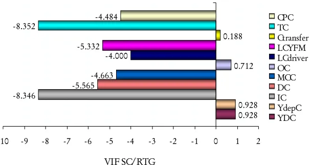
6.2 Cost comparison and sensitivity analysis using `VIF` values The values of cost comparison indicator, `R`, given in Table (6) have been used for calculation of `VIF` in this study. The following example demonstrates how the value of the variable intensity factors that favour a SC system over a semi-automated RTG system for different cost parameters, has been obtained. Consider that the initial cost of container yard equipment, `IC`, is the cost parameter that has been chosen as a preference attribute of comparison by a port operator. Then the `VIF` for a SC system over an RTG system with regard to the annual investment cost of both systems [Table (5)] which has been reflected by the `R` value (RSC/RTG = 1.162) obtained in Table 6.6 would be:
346 . 8 071 , 920 , 1 729 , 652 , 1 162 . 1 071 , 920 , 1
VIFSC/RTG − ≈− ×
=
The `VIF` for an RMG over an RTG system, where `RRMG/RTG =
0.750` with regard to the `LCdriver` would be:
250 . 2 000 , 675 000 , 900 750 . 0 000 , 675
VIFRMG/RTG − = ×
=
The `VIF` values for the SC over the semi automated RTG, the SC over the automated RMG and the automated RMG over the semi automated RTG have been calculated and summarised in Table (7).
Table (6) Variable intensity factor
Cost Parameter VIFSC/RTG VIFSC/RMG VIFRMG/RTG
LC - - - YDC 0.928 0.351 -5.081
YdepC 0.928 0.351 -5.081
YMC - - -
IC -8.346 -6.099 9.859
DC -5.565 -5.401 1.573
MCC -4.663 -4.020 2.703
OC 0.712 5.863 1.158
LCdriver -4.000 -4.267 2.250
LCYFM -5.332 -4.000 1.334
Ctransfer 0.188 0.092 -5.285
TC -8.352 -8.112 9.451
0.928 0.928
-8.346 -5.565
-4.663 0.712
-4.000
0.188
-8.352 -4.484
-5.332
-10 -9 -8 -7 -6 -5 -4 -3 -2 -1 0 1 2
1
VIF SC/RTG
CPC TC Ctransfer LCYFM LCdriver OC MCC DC IC YdepC YDC
Table (7) illustrates the `VIF` values of the systems discussed with the same sequence of preferences as indicated in `R` values. In the second column of the table, the VIFSC/RTG where a SC is considered to be
preferred over a semi-automated RTG system with regards to the `R` value and different cost parameters, it is evident that cost parameters for SC system such as `IC`, `DC`, `TC`, `LCdriver`, `LCYFM`, `MCC`and
`CPC` produce negative and the least values of `VIF`. They imply that a semi-automated RTG may be preferred over a SC system. In contrast `YDC`, `YdepC`, `OC` and `Ctransfer` cost factors have produced
positive values that may indicate the preferability and magnitude of `VIF` of a SC system over an RTG system. Figure (5) demonstrates the above statement where a SC system has not gained sufficient positive `VIF` values to override or even balance the negative values of `VIF` that imply the preference of an RTG over a SC system when the whole scenario is considered.
0.351 0.351 -6.099-5.401
-4.020 5.863
-4.267
0.092
-8.112 -4.122
-4.000
-9 -8 -7 -6 -5 -4 -3 -2 -1 0 1 2 3 4 5 6 7
1
VIF SC/RMG
CPC TC Ctransfer LCYFM LCdriver OC MCC DC IC YdepC YDC
In the third column of Table (7) and the corresponding illustration in Figure (6), it is demonstrated that `OC` has provided the highest positive `VIF` value for a SC system over an automated RMG system. Even though `YDC`, `YdepC` and `Ctransfer` cost attributes have also
provided additional positive values but the total positive value of the above parameters does not balance the total negative `VIF` value of `IC`,`DC`, `MCC`, `LCdriver`, `LCYFM`, `TC` and `CPC` parameters.
This implies the preferability of an automated RMG over SC system in this particular case.
Figure (6) Magnitude of VIFSC/RMG
From the forth column of Table (7) and the produced graph in Figure 6.7, it is evident that an automated RMG system has gained high positive `VIF` values in `TC`, `IC`, `CPC`, `LCdriver`, `MCC`,
`LCYFM`, `DC` and `OC` to favour an automated RMG over a
-5.081 -5.081
1.5732.703 2.250 -5.285
9.859 1.158
1.334
9.451 5.106
-7 -6 -5 -4 -3 -2 -1 0 1 2 3 4 5 6 7 8 9 10 11
1
VIF RMG/RTG
CPC TC Ctransfer LCYFM LCdriver OC MCC DC IC YdepC YDC
Figure (7) Magnitude of VIFRMG/RTG
7. Discussion
This study has developed a conceptual cost function model for the design and capacity of container terminals. The analysis of the test case has revealed that the size of a container yard, total containers to be processed, type, number and size of stacking cranes and transfer fleet and the costs associated with the procurement and maintenance of the cranes play a major role in the total cost and cost per container processed in a container yard.
The sensitivity analysis has indicated that cost parameters such as the transfer, operation, container yard development and container yard depreciation costs may favour selection of a SC system over a semi-automated RTG system. However, the evaluation and analysis have shown that cost parameters such as the initial cost of investment in the container yard equipment, equipment depreciation, maintenance and labour including total cost per container processed in a terminal favour the selection of a semi-automated RTG over a SC system.
crane depreciation, operation and maintenance cost of yard cranes together with crane manning and container yard foremen costs strongly support selection of an automated RMG over a semi-automated RTG system. According to the sensitivity analysis of this study, a semi-automated RTG system may also be preferred over an RMG system where the analysis shows lower transfer, development and depreciation cost parameters.
8. Conclusions and recommendations
This study has developed a generic model that helps to analyse, evaluate and measure the cost efficiency and effectiveness of the container yard operating systems proposed in a pair-wise manner. It has considered different cost functions used in modern container terminals. The size, annual throughput and mode of operation, the size and stacking height of container yard equipment together with cost parameters such as land cost, development, maintenance, operation, depreciation and procurement costs of container yard equipment and transfer vehicles and labour costs which are normally affected by automation technologies have been incorporated in the model. The model developed may enable the designer, planner and operator of a container terminal to set-up a comparison analysis platform for decision-making and to measure the impact of different cost parameters involved on the total cost of container yard operating systems. This study has proposed a sensitivity analysis tool using a cost comparison indicator and cost intensity factors for the analysis of cost efficiency in container terminals. The cost based model of this study provides the basis for pair-wise comparisons of container yard operating systems which is the main contribution of this study. Using a case study, the sensitivity analysis has demonstrated that an automated RMG system promises a lower cost per container, crane procurement and maintenance and container yard total costs than both RTG and SC systems.
operating systems. It should be noted that similar to the managers in the port industries, the managers and operators of other industries may resist revealing costs they have or are experiencing since high costs generally indicate the inefficiency and reduced productivity of systems.
9. Acknowledgments
References
1. Agerschou, H. (2004) Planning and Design of Ports and Marine Terminals, Thomas Telford Publication, London, pp. 274-286.
2. Avery, P. (1999) The Future of Cargo Handling Technology, Cargo Systems, IIR Publication Ltd. UK, pp. 38-44.
3. Bahrani, H. (2004) BACT Statistics, PSO, Bandar Abbas, Iran.
4. Chu, C. and Huang W. (2002-a) A Study on Ground Slot Layout and capacity of Container Yards, Journal of Maritime Quarter, No. 11, (Issue 4), pp. 15-34.
5. Chu, C. and Huang W. (2002-b) Land Planning of the Container Yards with Different Handling Systems, Journal of Maritime Research, No. 13, pp. 47-60.
6. Chu, C. and Huang W. (2003) Container Handling Capacity Study on Container Yards, Journal of Maritime Research, No. 14, pp. 29-44.
7. Constantinides, M. (1990) Economic Approach to Equipment Selection and Replacement, UNCTAD Monographs on Port Management, UNCTAD/Ship/494, (Issue 8), UN, New York, pp. 2-19. 8. Containerisation International (1990-2005) Ports, Journal of Containerisation International, Series from January 1990 to December 2005.
9. Containerisation International (1996) Market Analysis, In-terminal Handling Equipment, Journal of Containerisation International, April. 10. Guthrie, G. and Lemon, L. (2004) Mathematics of Interest Rates and Finance, Upper Saddle River, New Jersy, Prentice Hall.
11. Hatzitheodoroue, G. (1983) Cost Comparison of Container Handling Terminals, Journal of Waterways, Port, Coastal and Ocean Engineering, No. 109, (Issue 1), pp. 54-62.
12. Hee, K. and Wijbrands, R. (1988) Decision-Support Systems for Container Terminal Planning, International Journal of Operation Research, No. 34, pp. 262-272.
13. Kap, H. and Hong, B. (1998) The Optimal Determination of the Space Requirement and the Number of Transfer Cranes for Import Containers, Journal of Computer Industry Engineering, No. 35, (Issues 3 and 4), pp. 427-430.
Quayside Cranes, Journal of Marine Technology Society, Spring Edition, No. 40, (Issue 1), pp. 24-34.
15. Kiani, M., Bonsall, S., Wang, J. and Wall, A. (2006-b) A Break-even Model for Evaluating the Cost of Containerships’ Waiting-times and Berth Unproductive-Times in Automated Quayside Operations, The WMU Journal of Maritime Affairs, Vol. 5, No. 2 (October), pp. 153-179. 16. Kiani, M., Bonsall, S., Wang, J. and Wall, A. (2009) Application of Multiple Attribute Decision-Making (MADM) and Analytical Hierarchy Process (AHP) Methods in the Selection Decisions for a Container Yard Operating System, The Journal of Marine Technology Society, Volume 43, Number 3, August, pp. 34-50 (17).
17. Kiani, M. (2007) The Impact of Automation on the Efficiency and Cost Effectiveness of the Quayside and Container Yard Cranes and the Selection Decision for the Yard Operating Systems, PhD Thesis, School of Engineering, Liverpool John Moores University, UK.
18. Kim, K. and Kim, H. (2002) The optimal sizing of the storage space and handling facilities for import containers, Journal of Transportation Research -B, No. 36, pp. 821-835.
19. Kim, K. and Kim, H. (1998) The Optimal Determination of the Space Requirement and the Number of Transfer Cranes for Import Containers, Journal of Computer and Industrial Engineering, No. 35, pp. 427-430.
20. Liu, C., Jula, H. and Ioannou, P. (2002) Design, Simulation and Evaluation of Automated Container Terminals, Journal of IEEE
Transactions on Intelligent Transportation Systems, No. 3, (Issue 1), pp. 12-26.
21. Nahavandi, N. (1996) Design Model for Loading, Unloading and Storage of Container Ports, M.Sc. Dissertation, Amir Kabir University of Technology, Iran, pp. 55-70.
22. Nam, K. and Ha, W. (2001) Evaluation of Handling Systems for Container Terminals, Journal of Waterways, Port, Coastal and Ocean Engineering, No. 127, (Issue 3), pp. 171-175.
Technical Report, Presented in the Section System Engineering Seminar, 26-29th October, Netherlands, Delft University of Technology, pp. 577-84. 25. Steiner, H. (1992) Engineering Economic Principles, McGraw- Hill, New York, USA, pp. 317-490.
26. Thuesen, G. and Fabrycky, W. (1993) Engineering Economy, Prentice Hall, Englewood Cliffs, Newjercy, USA, pp. 273-486.
27. UNCTAD, (1985) Port Development, A handbook for Planners in Developing Countries, UNCTAD, TD/B/C. 4/175/rev.1, UN, New York, pp. 17-33.
28. UNCTAD, (1990-2005) Review of Maritime Transport, UNCTAD Publications, Series from 1990 to 2005.
29. UNCTAD, (2002) How to Prepare Your Business Plan, UNCTAD/ITE/IIA/5, UN, New York and Geneva, pp. 139-182.
30. UNCTAD, (2005) Review of Maritime Transport, UN, New York and Geneva, pp. 19-55.
31. Vis, I. and Harika, I. (2004) Comparison of Vehicle Types at an Automated Container Terminal, Journal of Operation Research Spectrum, No. 26, (Issue 1), pp.117-143.
32. Watanabe, I. (1995) An Analysis of Size of Container Handling Equipment Fleet Required for Receiving and Delivering Operations in Container Terminals, 9th Terminal Operations Conference, Singapore. 33. Watanabe, I. (2001) Container Terminal Planning, a Theoretical Approach, World Cargo Publishing, Leatherhead, UK.
34. World Port Development International, (1990-2006) Container Handling Equipment, International Journal of World Port Development, Series from January 1990 to September 2006.
35. Yang, C., Choi, Y. and Ha, T. (2004) Simulation Based Performance Evaluation of Transport Vehicles at Automated Container Terminals, Journal of Operation Research Spectrum, No. 26, (Issue 2), pp. 149-170. 36. Zahiri, H. (2005) The Potentials for Transit of Goods in Iran, Economic-Scientific Journal of Payam-e-Darya, Iran, July, No. 4, (Issue 35), pp. 17-25.
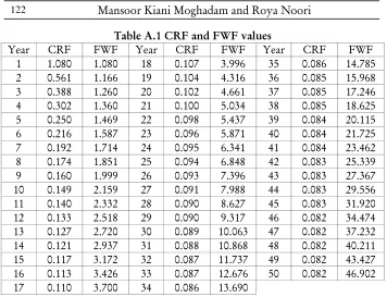
Appendix (1) CRF and FWF values
CRF
A Capital Recovery Factor (CRF) is defined as the ratio of a constant annuity to the present value of receiving that annuity for a given length of time. Using an average interest rate `i` and number of annuities received `t`, the capital recovery factor converts a total amount of investment into an annuity amount of equal series. The CRF can be calculated from the following equation:
( )
( )
1 it 1t i 1 i CRF
− +
+ × =
where:
t = Number of project life and i = Average interest rate.
If `t = 1`, then CRF reduces to `1+i`. As `t` goes to infinity, the CRF goes to `i`. In this context, an annual cost of an investment can be expressed as follows:
P(IC) = IC x CRF where:
P(IC) = Annual cost of investment. IC = Initial cost of investment.
On the basis of the above statements, a total cost of an investment [TP(IC)] may be defined as:
TP(IC) = P(IC) x t.
FWF
A Future Worth Factor (FWF) converts a present value of an investment into a future amount using an average interest rate `i` and number of economic life in years expected from a project `t`. The FWF = (1+i)t-1. In this context `1/ (1+i)t-1` would be a Present Worth Factor
Table A.1 CRF and FWF values