1- Introduction
Large-scale interconnected systems are applied in numerous fields, including electrical power systems, chemical reactors, economic systems and computer communication networks. In recent decades, scientific researchers have focused on the decentralized control of large-scale systems and many results have been obtained [1]. The information exchange among subsystems of large-scale interconnected systems through communication networks unavoidably causes time delays. Thus, investigation of decentralized control problems of nonlinear interconnected systems with time delays is of high importance [2]. It should be noted that evaluating a time delay system is complex because of infinite dimension [3]. It has been reported that MRAC is an effective method for controlling systems with uncertainties and delays (see e.g. [4, 8, 16]).
In many practical control problems, the parameters and the dynamics of the original system are unknown, but the upper bounds may be unknown or partially known. Therefore, adaptive schemes must be adopted to update the partially known bounds of uncertainty for uncertain large-scale systems that are dynamically interconnected and suffer from time delays. In [5], the plant model with linear interconnections was considered where the nonlinear local inputs are bounded with unknown bounds, and then an adaptive controller was designed for the model. In [6], the plant includes uncertain delayed nonlinear interconnections bounded by a known function, and there is, therefore, no adaptation law. Decentralized adaptive controllers have been applied to uncertain large scale time-delay interconnected systems [7, 19]. The nonlinear interconnection terms are generally assumed to be bounded by the linear functions of the norm of the states [8]. It is notable that in some recent works, the nonlinear interconnection terms are assumed to be
Corresponding author; Email: [email protected]
bounded to the related states by a higher-order polynomial [9]. It has been found that so many researchers have focused on adaptive control of large scale systems [4, 7, 8, 18], but the key issue of input delay which is important in practical applications has not been investigated.
For a linear system with pure input delay, Smith predictor is introduced in [10]. However, if the open-loop system is unstable, the Smith predictor may fail to stabilize the overall system. The limitation on the open-loop stability required by the Smith predictor in the input delay compensation can be removed by the use of a new approach called the predictor feedback [11]. The idea behind this approach is to apply the future state which can be estimated from the current state and the past control signals, in order to compensate for the input delay. A good feature of the mentioned method is that the closed-loop system has only a finite number of zeroes. Hence, this method is also known as the finite spectrum assignment [11]. Linear systems with both input and state delays have been investigated, and a sliding mode control scheme to achieve stabilization has been presented in [12]. A finite dimensional feedback control law that is truncated from the traditional predictor feedback proposed in [13], based on the low gain feedback structure [14]. To tackle the problems of implementation of predictor feedback controllers for input delayed systems, truncated predictor feedback method was introduced for systems with delays in their input and states [15]. Also, Smith predictor method is applied to systems with both state and input delays in [16]. For the delay compensation, two auxiliary dynamic adaptive filters with adjustable gains were included in the adaptive controller part. However, due to existence of these filters, the tracking error could not be minimized. The nested predictor is another method which has been presented for state and input delays compensation [17] for system stabilizing problems. The largescale systems with delay in interconnection terms were investigated in [8] with no input delay. Also, the control law proposed in [8] is very AUT J. Model. Simul., 50(1)(2018)3-12
DOI: 10.22060/miscj.2017.12239.5021
Decentralized Model Reference Adaptive Control of Large Scale Interconnected
Systems with Both State and Input Delays
S. H. Hashemipour1, N. Vasegh2, A. Khaki Sedigh3
1 Department of Electrical Engineering, Roudsar and Amlash Branch, Islamic Azad University, Roudsar, Iran. 2 Department of Electrical Engineering, ShahidRajaee Teacher Training University, Tehran, Iran.
3 Department of Electrical Engineering, K. N Toosi University of Technology, Tehran, Iran.
ABSTRACT: In this paper, the problem of decentralized Model Reference Adaptive Control (MRAC) for interconnected large scale systems associated with time varying delays in state and input is investigated. The upper bounds of the interconnection terms are considered to be unknown. Time varying delays in the nonlinear interconnection terms are bounded and non-negative continuous functions and their derivatives are not necessarily less than one. Moreover, a simple and practical method based on periodic characteristics of the reference model is established to predict the future states and input delay compensation. It is shown that the solution of uncertain large-scale time-delay interconnected system converges uniformly exponentially to inside of a desired small ball. Simulation results of a chemical reactor system and a numerical example illustrate effectiveness of the proposed methods.
Review History:
Received: 10 December 2016 Revised: 19 May 2017 Accepted: 22 May 2017 Available Online: 25 July 2017 Keywords:
Interconnected system MRAC
complex and not applicable to practical systems. In [19], the interconnected system without any delay in inputs and states was considered.
In this paper, a decentralized MRAC is designed for a large-scale interconnected system subject to time-varying input and state delays in terms of a nonlinear interconnection. The controller is designed in two steps. In the first step, a simple and practical method is applied to predict the future states for compensation of input delays. For the prediction of the periodic characteristics of the reference model states are used. In the next step, by assuming that the state x(t+R) is predicted, the adaptive controller will be designed. Also, it was assumed that the time varying delays are any non- negative continuous and bounded functions. It is not necessary to have their derivatives being less than one, and, moreover, the nonlinear interconnection terms, which also include time-varying delays, are bounded with unknown non- negative nonlinear functions that not requirement to be known for the design. The paper is organized as follows. In section 2, problem formulation and assumptions are introduced. The controller design and system stability proof are given in section 3. Simulation results of a chemical reactor system and a numerical example are given in section 4. The final section concludes the paper.
2- Problem formulation and assumptions
Consider a class of large scale systems composed of N
interconnected subsystems with delays in states and inputs, described by the following equations:
(
)
1
: ( ) ( ) ( ) ( )
( ( )), ( )
i i i i di i i i i i
N
i ij j ij ij
j
S x t A x t A x t d B u t R B ξ x t h t t h t
=
= + − + −
+
∑
− −
(1)
where ∈ℜni
i
x and ∈ℜmi
i
u represent the state and control vectors of the i-th subsystem, respectively; Ai, i i
i
n n d
A ∈ℜ × and ∈ℜn mi× i
i
B are known as constant matrices, di and Ri
indicate constant delays, and ξij
(
x t h t t h tj( − ij( )), − ij( ))
are uncertain interconnections, which represent the interconnections between the present and delayed states of systems Si and Sj , and hij(t) denote the differentiable and bounded time varying delay that satisfy0≤fij ≤h tij( )≤hij < ∞. (2)
where fij and hij are positive constants. In the control literature [8, 9], it is generally assumed that hij(t) are positive and their derivatives are less than one. In this paper, we eliminate the differentiability condition. Hence, let hij(t) be positive continuous bounded functions which do not require to be known. The initial conditions are
[
0 0]
( ) ( ), , , 1,2,..., .
i i i
x t = Ξ t t∈ t −τ t i = N
where τi =max
{
h dij, i}
and ( )Ξi t are continuous functions. The stable non- delayed reference model is defined by the differential equation as( ) ( ) ( )
mi mi mi mi i
x t =A x t +B D t (3) where ∈ℜni
mi
x is the state vector, Di(t) is periodic and the piecewise continuous reference input to the i-th reference model. Ami and Bmi are known matrices.
To system (1) and model reference system (3), the following assumptions are given.
Assumption 1.There is the positive definite matrix Pi that satisfy the following equations
, 1,2,..., ,
T
mi i i mi i
A P P A+ = − =Q i N (4) where Qi are positive definite matrices.
Assumption 2. There are the constant vectors ni, ni
i i
z ∈ℜ m ∈ℜ
,
i i
n n
i i
z ∈ℜ and a non-zero scalar m ∈ℜ θri that satisfy the following equations,
, 0,
i mi i i di i i mi i ri
A A− =B z A +B m = B =B
θ
.Assumption3.The nonlinear interconnection term
ξ
ij(.)satisfies the following inequality
(
( ( )), ( ))
( ) (
* T ( ( )), ( ))
ij x t h t t h tj ij ij ij ij x t h t t h tj ij ij
ξ − − ≤ θ ρ − − (5)
where
1 2
(.) (.) (.) ... j(.) T
ij ij ij ijl
ρ = ρ ρ ρ
and
* * * *
1(.) 2(.) ... j(.)
T
ij ij ij ijl
θ = θ θ θ
are the upper bound nonlinear function and an unknown constant vector, respectively. It is assumed that
ρ
jik(.) 0>for =k 1,2,..., ,lj and these functions are continuous and uniformly bounded with respect to the state xj and the time
t [19].
Assumption 4.All subsystems are stable.
Remark 1.Assumption 1 will be always satisfied if the pair {Ami, Bi} is stable and controllable. The so-called matching condition widely employed in the strenuous filtering and controlling problems satisfy Assumption 2 (see [9, 16]).
Remark 2. The interconnection terms are generally considered to be linear or the states are bounded by linear norms in the literature. In some works, the nonlinear interconnection terms are assumed to be bounded by a higher-order polynomial of states variables [9]. Here we assume that the interconnection term is bounded by a function that is described in Assumption 3. Moreover, the proposed decentralized control schemes are completely independent of the function ρij(·) that is not required to be known.Let
{
}
2
* 1 *
1
1 , 1,2,...,
2 N
i i ij ij
j
i N
ϕ η ε θ−
=
=
∑
∈ (6) where ηi andε
ij are positive constants, andε
ijis notnecessarily known. It is clear from Assumption 3 that
ϕ
i*isan unknown positive constant. 3- Controller Design
In this section, first, a simple and practical method based on periodic characteristics of the reference model is introduced to predict the future states and to compensate the input delays. Then, by using the state x(t+R), a decentralized adaptive feedback controller is designed. However, this method can be used only when the reference input is periodic and continuous and subsystems are stable.
3- 1- Calculation of the future states x(t+R) By definition, periodic signal is as follows:
( ) ( ) ( )
where β is a positive integer. Let T R b
β = + (8) where b≥0 and β =1 if T≥R, and β >1, otherwise.
Thus, by a time delay, signal x(t+R) can be produced. By using (7) and (8), we will have
( ) ( ) ( )
x t =x t +βT =x t R b+ + (9) and then
( ) ( )
x t b− =x t R+ (10)
This relation shows that using the periodicity property, time delay can be used instead of prediction. This simple and practical feature can be applied to reduce the effect of interconnection term in the design MRAC for the large scale system.
3- 2- Model reference adaptive controller design
A decentralized adaptive feedback controller is designed for system (1) which satisfies the above Assumptions. Our goal is to ensure that all the closed loop signals remain bounded and the tracking error becomes small enough. The tracking error is defined as
( )= ( )− ( )
i i mi
e t x t x t (11) The error’s dynamics is obtained as
(12)
(
)
1
( ) ( ) ( ) ( )
( ( )), ( ) ( ) ( )
i i i di i i i i i
N
i ij j ij ij mi mi mi i
j
e t A x t A x t d B u t R
B ξ x t h t t h t A x t B D t =
= + − + − +
− − − −
∑
The main results are presented in the following theorem. Theorem 1. Consider system (1), let the decentralized adaptive feedback controller be designed as
1 2
( ) ( ) ( )
i i i
u t =u t +u t (13) where
1( ) ( ) ( ) ( ),
i i i i ri i i i i i i
u t = −z x t R+ +θ D t R+ +m x t R d+ − (14)
2( ) 1 ˆ2 ( ) T ( )
i i i i mi i i i
u t = − η ϕ t R B P e t R+ + (15)
and ηi are positive constants.
If ˆϕi are the estimates of the unknown *
i
ϕ
and are obtained by (16), then2
ˆ (i i) ˆ( ) T ( ) . i i i i i mi i i i
d t R t R B P e t R
dt
ϕ + γ σ ϕ η γ
= − + + + (16)
If we define ( ) ˆ( ) *
i t Ri i t Ri i
ϕ + =ϕ + −ϕ , (16) can be written as
2 *
( ) ( )
+ ( )
i i
i i i
T
i i mi i i i i i i
d t R t R
dt
B P e t R
ϕ γ σ ϕ η γ γ σ ϕ + = − + + + − (17)
where γi and σi are any given positive constants, and
0
ˆ ( )i t
ϕ is finite. Moreover, let
( ) ( ) ( ),
i i i i mi i
e t R+ =x t R+ −x t R+ (18)
where xi(t+Ri) can be obtained by applying time delay to periodic state xi(t), and x t Rmi( + i) can be obtained by applying the input D t Ri( + i) to (3). Then, the tracking error converges uniformly exponentially towards a ball, and the large scale system is stable.
Proof.Define the following Lyapunov function as: (19)
{
}
1 2 1 ( ( ), ( )) ( ) ( ) ( ) , 2 1,2,..., . Ti i i ri i i i i i
V e t t e t P e t t
i N
ϕ =θ + γ ϕ−
=
where matrices Pi satisfying (4) are positive definite and i
γ are positive constants. It is proved that the tracking error ei(t) converges uniformly exponentially towards a ball which is as small as desired in the presence of the nonlinear interconnected term.
Equation (12) can be written as
(
)
1
( ) ( ) ( ) ( ) ( ) ( )
( ) ( ( )), ( ) .
i mi i i mi i di i i mi i
N
i i i i ij j ij ij
j
e t A e t A A x t A x t d B D t
B u t R B ξ x t h t t h t =
= + − + − −
+ − +
∑
− −
(20) By Assumption 2 and equation (13), (20) can be rewritten as
(21)
(
)
(
)
1 2 1 ( ) ( ) ( ) ( ) ( ) ( ) ( ) ( ( )), ( ) ,i mi i i i i i i i i
mi i i i i i i
N
i ij j ij ij
j
e t A e t B z x t B m x t d B D t B u t R u t R
B ξ x t h t t h t =
= + − − −
− + − + − +
+
∑
− −
and after inserting (14) in (21), we have
(
)
2
1
( ) ( ) ( )
+ ( ( )), ( ) .
i mi i i i i
N
i ij j ij ij
j
e t A e t B u t R
B ξ x t h t t h t = = + − + − −
∑
(22)By taking the time derivative of V (.) , and using (22) and i
(15), we have
(
)
(
)
1
2 1
( ( ), ( )) ( ) ( )
+ 2 ( ) ( ( )), ( )
( ) ˆ
( ) ( ) ( ) .
T T i i i
ri i mi i i mi i N
T
i i mi ij j ij ij j
T i
i i mi i i i i
dV e t t e t A P P A e t dt
e t PB x t h t t h t
d t t B P e t t
dt ϕ θ ξ ϕ η ϕ γ ϕ = − = + + − − − +
∑
(23)By using (4) and (5), above equation can be written for any
t≥t0,
( ) (
)
2 min * 1 2 1 ( ( ), ( )) ( ) ( )+2 ( ) ( ( )), ( )
( ) ˆ
( ) ( ) ( )
i i i
ri i i
N T
T
mi i i ij ij j ij ij j
T i
i i mi i i i i
dV e t t Q e t
dt
B Pe t x t h t t h t
d t t B P e t t
dt ϕ θ λ θ ρ ϕ η ϕ γ ϕ = − ≤ − + − − − +
∑
(24)According to [19] and the Lyapunov stability theory i.e. for each positive constant ε >0
1
2X YT ≤εX XT +ε−Y YT ,∀X Y, ∈Rn (25)
From (24) and (25) and the definition of the parameter
ϕ
i* in(6), we have for any t≥t0,
(
)
(26)2 min 2 2 1 * 1 2 1 ( ( ), ( )) ( ) ( ) + ( ( )), ( ) ( ) ( ) ˆ ( ) ( ) ( )
i i i
ri i i
N
T
j ij j ij ij i i mi i i
j
T i
i i mi i i i i
dV e t t Q e t
dt
x t h t t h t B P e t
d t
t B P e t t
Since
ϕ
i( )t =ϕ
ˆi( )t −ϕ
i*, it holds that (27)(
)
2 min 21 2 *
1
( ( ), ( )) ( ) ( )
( ( )), ( ) ( ) ( )
i i i
ri i i N
j ij j ij ij i i i i i
j
dV e t t Q e t
dt
x t h t t h t t t
ϕ θ λ ε− ρ σ ϕ σ ϕ ϕ = ≤ − + − − − −
∑
If we use the inequality
( )
22 * 1 2 1 *
( ) ( ) ( )
2 2
i i t i i t i i i t i i
σ ϕ σ ϕ ϕ σ ϕ σ ϕ
− − ≤ − + , (28)
one can say that
(29)
(
)
( )
2 min 2 21 2 *
1
( ( ), ( )) ( ) ( )
1 1
+ ( ( )), ( ) ( )
2 2
i i i
ri i i
N
j ij j ij ij i i i i
j
dV e t t Q e t
dt
x t h t t h t t
ϕ θ λ ε− ρ σ ϕ σ ϕ = ≤ − + − − − +
∑
Regardless of the negative terms, by using (19) and (29) for any t≥t0, it can be written as
(30)
(
)
( )
min 2 2 1 * 1 ( ( ), ( )) ( ( ), ( )) 1 ( ( )), ( ) 2i i i
i i i
N
j ij j ij ij i i
j
dV e t t V e t t
dt
x t h t t h t
ϕ µ ϕ ε ρ− σ ϕ = ≤ − +
∑
− − + where{
1}
min min min( ) max( ),
i Qi Pi i i
µ = λ λ− σ γ
(31) Let V ti( )=V e t( ( ), ( ))i ϕi t , by the definition of
( ( ), ( )) i i i
V e t ϕ t given by (19) , following [19], and using (31), we have for any t≥t0,
(32)
( )
(
)
(
)
min 0 min 02 1 ( )
min 0
2
1 1 *
min min 2 ( ) 1 1 min 1 ( ) ( ( )) ( ) 1 ( ( )) 2 ( ( )) ( ( )), ( ) i i t t
i ri i i
ri i i i i
N t
t
ri i ij t ij i ij ij
j
e t P e V t
P
P e x h h d
µ µ τ θ λ θ λ µ σ ϕ θ λ ε ρ τ τ τ τ τ − − − − − − − − − = ≤ + + + − −
∑
∫
whereεij, j∈
{
1,2,...,N}
are positive constants. Thus, the following inequality can be written as(
)
1 1min 1 min ( ) 1 i N
ri i ij
j P θ λ ε µ − − = <
∑
(33)Now, according to [19], for any 0≤δi ≤µimin, the following
continuous function is defined as
(
)
1 1min
1 min
( )
( ) i ij
N
h
ri i ij
i
j i i
P
k δ θ λ ε eδ
µ δ
− −
= =
−
∑
(34)It is obvious from (33) that k(0)<1. Therefore, there are a δ >0i 0 that the inequality 0<δ0i <µimin holds and
0
( ) 1i
k δ < such that
0i ( ) 10i
k =k δ < (35) Now, multiplying both sides of (32) byeδ0i(t t−0), we have for any t≥t0,
( )
(
)
(
)
(
)
(
)
(
)
0 0
0 0
0 0 0
min 0 0
2 ( ) 1
min 0
2 ( )
1 1 *
min min 2 ( ) ( ( ) ) ( )( ) 1 1 min ( ) ( ( )) ( ) 1 +( ( )) 2 ( ( )) ( ( )), ( ) i i
i ij i ij
i i
t t
i ri i i
t t
ri i i i i
t t h h t
ri i ij t ij j ij ij
j
e t e P V t
P e
P e e x h h e d
δ δ δ τ δ τ τ µ δ τ θ λ θ λ µ σ ϕ θ λ ε ρ τ τ τ τ τ − − − − − − − − − − − − = ≤ + +
∫
− − 1 N∑
(36)( )
(
)
(
)
(
)
(
)
(
)
0 0 0 00 0 0
min 0 0
2 ( ) 1
min 0
2 ( )
1 1 *
min min 2 ( ) ( ( ) ) ( )( ) 1 1 min ( ) ( ( )) ( ) 1 +( ( )) 2 ( ( )) ( ( )), ( ) i i
i ij i ij
i i
t t
i ri i i
t t
ri i i i i
t t h h t
ri i ij t ij j ij ij
j
e t e P V t
P e
P e e x h h e d
δ δ δ τ δ τ τ µ δ τ θ λ θ λ µ σ ϕ θ λ ε ρ τ τ τ τ τ − − − − − − − − − − − − = ≤ + + − −
∫
1 N∑
For any t≥t0, let
(
0 0)
0
2 ( )
0 ( ) max, ( ) i
ij
t
i t h t i
Y t e eδ ζ
ζ ζ
−
∈ −
= (37) and
(
0 0)
0
2 ( )
,
( ) max ( ( ), ) i
ij
t ij t h t ij j
S t x eδ ζ
ζ ρ ζ ζ
−
∈ −
′ = (38)
Then, it can be obtained from (36) that for any t R∈ +,
(
)
( )
0 0 0 0 0 1 12 ( ) 1 min
min 0
1 min 0 2 ( )
1 1 *
min min ( ) ( ) ( ( )) ( ) ( ) 1 ( ( )) 2 i ij i i N h
ri i ij
t t
i ri i i ij
j i i
t t
ri i i i i
P
e t e P V t e S t
P e δ δ δ θ λ ε θ λ µ δ θ λ µ σ ϕ − − − − = − − − ′ ≤ + − +
∑
(39)It is clear from (37) and (38) that S tij′( ) are non-decreasing
functions. The right–hand side of the inequality (39) is also non-decreasing. Thus, using (39) and Y0i(t) in (37), we have:
( )
( )
0 0
0
2 ( )
1 1 1 *
0 min 0 min min
1 1 min
1 min 0
1
( ) ( ( )) ( ) ( ( )) 2
( )
( )
i
i ij
t t
i ri i i ri i i i i
N h
ri i ij
ij
j i i
Y t P V t P e
P
e S t
δ δ θ λ θ λ µ σ ϕ θ λ ε µ δ − − − − − − = ≤ + ′ + −
∑
(40)If we take
{
0}
( ) max ( ), ( ) , , 1,2,..., , 0
i i ij
S t′ = Y t S t′ i j = N t ≥ (41) and using (34) and (35), the equation (40) is given by the following inequality,
( )
0 01
0 min 0 0
2 ( )
1 1 *
min min
( ) ( ( )) ( ) ( ) 1
( ( )) .
2 i
i ri i i i i
t t
ri i i i i
Y t P V t d S t
P eδ
θ λ θ λ µ σ ϕ − − − − ′ ≤ + + + (42)
As Y0i(t) and S’i(t) are non-decreasing functions and
ε
ij arepositive, then as in [19],
*
0i i( ) i 0i( )
d S t′ ≤υY t (43) where
υ
i*<1 is any given positive constant. Moreover, forthe designer, it is not necessary to choose or know εij (see
Remark 3).
By inserting (43) into (42), we have
( )
0 01 *
0 min 0 0
2 ( )
1 1 *
min min
( ) ( ( )) ( ) ( )
1
+( ( )) .
2 i
i ri i i i i
t t
ri i i i i
Y t P V t Y t
P eδ
θ λ υ θ λ µ σ ϕ − − − − ≤ + + (44) Then,
( )
0 01 min
0 * 0
1 1 2
( ) * min min * ( ( )) ( ) ( ) 1
( ( )) 1
+ 2 1 i ri i i i i t t
ri i i
i i i
P
Y t V t
By the definition of Y0i(t) in (37), we have
0 0
2 ( )
0
( ) ( ) i t t
i i
e t ≤Y t e−δ − (46) Therefore,
( )
0 0
1
2 min ( )
0 *
1 1 2
* min min * ( ( )) ( ) ( ) 1
( ( )) 1
2 1
it t ri i
i i
i
ri i i
i i i
P
e t V t e
P δ θ λ υ θ λ µ σ ϕ υ − − − − − ≤ − + − (47) and [ ) 0 0 0 1 1 ( ) min min 0 0 * * , ( ( )) ( ( ))
sup ( ) ( ).
1 it t 1
ri i ri i
i i
t i i
P V t eδ P V t
θ λ θ λ υ υ − − − − ∈ ∞ ≤ − −
(48)
The norm e t i( ) in (47) is uniformly bounded, and it converges uniformly exponentially to B c( )0i where
( )
1 1 2
* min min
0 0 *
( ( )) 1
( ) ( ) .
2 1
ri i i
i i i i i i
i
P
B c e e t c θ λ µ σ ϕ
υ − − = ≤ = −
(49)
Because the estimated value ϕˆ ( )i t in (16) is uniformly bounded, the tracking error e ti( ) is bounded, and the proof is complete.
Remark 3. Since the adaptive control law in (16) is independent of εij , it is not necessary for the designer to know or choose these positive constants. (More details can be found in [19]).
4- Numerical Examples
In this section, to show the effectiveness of the proposed approach, a numerical example and a chemical reactor system are presented.
Example 1. Consider a large-scale system with
time-varying state and input delays, the two subsystems of which are described as follows:
1 2
1 1 1 1 1 1
2
0.5 ( ( )) 0.6 ( ( ))
1 1
2 2 2 2 2 2
1 1 0 0 0
( ) ( ) ( ) ( )
2 3 2 3 1
0
( ) 1
1 1 0 0 0
( ) ( ) ( ) ( )
3 3 2 3 1
j ij j ij
x t h t x t h t j
j
x t x t x t d u t R
t e
x t x t x t d u t R
ζ − + − = − = + − + − − − − − + − = + − + − − − − −
∑
1 20.5 ( ( )) 0.6 ( ( ))
2 1
0
+ 1 N ( ) x t h tj ij xj t h tij )
j j t e ζ − + − =
∑
(50)where
ζ
ij( )t are unknown that not requirement to be knownfor the design.
To design the adaptive controller, the reference model is selected as
1 1 1
2 2 2
1 1 0
( ) ( ) ( )
6 5 1
1 1 0
( ) ( ) ( )
7 5 1
m m
m m
x t x t D t
x t x t D t
− = + − − − = + − −
(51)
where
1( ) 10sin4 , 2( ) 10cos4 .
D t = πt D t = πt
Therefore, by Theorem 1, the controllers are
[
]
[
]
1 1 1 1 1 1
1 1 1 1 1 1 1 1 1
( ) 4 2 ( ) 2 3 ( )
1 ˆ
( ) ( ) ( )
2
T m
u t x t R x t d R
D t R η ϕ t R B P e t R
= − − + + − +
+ + − + + (52)
[
]
[
]
2 2 2 2 2 2
2 2 2 2 2 2 2 2 2
( ) 4 2 ( ) 2 3 ( )
1 ˆ
( ) ( ) ( )
2 mT
u t x t R x t d R
D t R η ϕ t R B P e t R
= − − + + − +
+ + − + + (53)
and the adaptive laws are
2
ˆ (i i) ˆ( ) T ( ) i i i i i mi i i i
d t R t R B P e t R
dt
ϕ + γ σ ϕ η γ
= − + + + (54)
with
( ) ( ) ( )
i i i i mi i
e t R+ =x t R+ −x t R+ (55) The future states x t Rmi( + i) can be obtained by applying the input D t Ri( + i) in (51). Also, the state x t Ri( + i) can be predicted by the method introduced in section 3.1.
The parameter values of the controller are chosen as:
1 2 1 2
1 2
1 2
1, 3.4, 2, 5, 0.1,
( ) 0.2sin(3 ), ( ) 0.3sin(3 ), 10 ,
( ) 1 0.5sin( ), ( ) 1 0.4sin( ).
i i i
j j i
i i
d d R R
t t t t Q I
h t t h t t
η γ σ ζ ζ π π = = = = = = = = = = = + = +
hi1(t) and hi2(t) are bounded continuous functions and their derivatives are not necessarily less than one. Also, in the controller design, it does not need to be known. The initial conditions are
1 0
(0) , (0) .
1 0
i mi
x = − x =
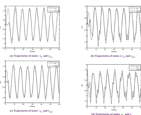
Simulation results are shown below. Figure 1 shows the plant and reference model’s states xi(t) and xmi(t), and Figure 2 shows the errors ei(t) and the control signal.
Example 2. We consider a chemical reactor recycle system that was presented in [8] but the input delay is added to it. This example is a large scale model composed of two subsystemsas:
(56)
0.5 1 0 0.5 0.5 0
0 0.5 1 0 0.5 0.5 ( ) 0 0 0.5 0.5 0.5 0.25
0 0
0 ( ) 0 ( ), 1,2.
1 1
i i i i
i i i
x x x t d
u t R f t i
− − − = − + − − − − − + − + =
where the uncertain nonlinear functions are chosen as
(57)
1 1 1 2 11
2
1 1 11 2 12 13 1
2 2 2 1 21
2
2 2 21 1 22 23 2
( )
( ) (
( ))
(
( )) (
( ))
(
)
( )
( ) (
( ))
(
( )) (
( ))
(
)
T T T Tf t
x t x t h t
x t h t x t h t
x t d
f t
x t x t h t
x t h t x t h t
x t d
µ
µ
µ
µ
=
−
+
−
−
−
−
=
−
+
−
−
−
−
that
µ
1 andµ
2 are unknown parameters. To design the0 10 20 30 40 50 60 -2.5
-2 -1.5 -1 -0.5 0 0.5 1 1.5 2
Time(s)
x11
x11 xm11
(a) Trajectories of states x11 and xm11
0 10 20 30 40 50 60
-2 -1.5 -1 -0.5 0 0.5 1 1.5 2
Time(s)
x21
x21 xm21
(c) Trajectories of states x21 and xm21
0 10 20 30 40 50 60
-2 -1.5 -1 -0.5 0 0.5 1 1.5
Time(s)
x12
x12 xm12
(b) Trajectories of states e x12 and xm12
0 10 20 30 40 50 60
-2 -1.5 -1 -0.5 0 0.5 1 1.5 2
Time(s)
x22
x22 xm22
(d) Trajectories of states x22 and xm22
0 10 20 30 40 50 60
-1 0 1 2
Time(s)
u1
0 10 20 30 40 50 60
-1 -0.5 0 0.5 1
Time(s)
u2
(a) Control signals u1 and u2
0 10 20 30 40 50 60
-2 -1 0 1 2
Time(s)
e1
e11 e12
0 10 20 30 40 50 60
-2 -1 0 1 2
Time(s)
e2
e21 e22
(b) Error signals e1 and e2
Figure 1. Time responses of states and model references
0.5 1 0 0
0 0.5 1 0 ( ), 1,2,
0 0 1
mi mi i
i
x x D t i
a −
= − + =
−
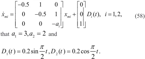
(58)
that
a
1=
3,
a
2=
2
and1( ) 0.2sin
2
, ( ) 0.2cos22
.D t =
π
t D t =π
tThe interconnected term in (57) can be bounded by a higher-order polynomial, however using the method presented in this paper, the interconnected term is only assumed bounded with an unknown function. Therefore, by theorem 1, the controllers are
(59)
[
]
[
]
1 1 1
1 1 1
1 1 1 1 1 1 1 1 1
( ) 0 0 1.5 ( )
+ 0.5 0.5 0.25 ( )
1 ˆ
( ) ( ) ( )
2 Tm
u t x t R
x t R d
D t R
ηψ
t R B P e t R= + +
− − + −
′
+ + − + +
(60)2
[
[
]
2 2]
2 2 2
2 2 2 2 2 2 2 2 2
( ) 0 0 2.5 (
)
+ 0.5
0.5 0.25 (
)
1 ˆ
(
)
(
)
(
)
2
T m
u t
x t R
x t R d
D t R
η ψ
t R B P e t R
=
+
+
−
−
+
−
′
+
+
−
+
+
As mentioned, for the prediction of the periodic characteristics of the reference model states are used. The system received reference input by the control law (14) and, therefore, the states of system are periodic, thus,
(
)
( 4)
( )
x t T
+
=
x t
+
=
x t
(61) Using (10), above equation can be written as(
)
( 0.4)
( 3.6)
x t R
+
=
x t
+
=
x t
−
(62)Also, adaptive law and tracing error are similar in (54) and (55), respectively. The parameter values of the controller are
chosen as:
(
)
1 2 0.3, 0.4, 0.5, ( ) 0.2 1 sin ,
10 , 7, 4, 0.1.
i i ij
i i i i
d d R h t t
Q I
µ
γ
η
σ
= = = = = +
= = = =
The initial conditions are
1 2
1
0.8
(0)
0
, (0)
0
1
0.8
x
x
=
=
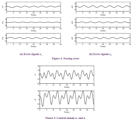
With the designed controller, Figure 3 shows the plant and reference model states, i.e. xi(t) and xmi(t), respectively, and Figures 4 and 5 show the errors ei(t) and the control signal. with the designed controllers, the states of the closed loop system are illustrated in the results. it can be seen for the system (50) and (56) and with both state and input delay and nonlinear interconnected terms with time varying delays, the tracking error converges uniformly exponentially to a ball. 5- Conclusion
In this research, the MRAC problem was investigated for a large scale system with both state and input delay and nonlinear interconnected terms. Delay in the input is compensated by a simple and practical method based on the periodic characteristics of the reference model. Also, it is considered that the upper bounds of the uncertainties in the interconnection terms are unknown. Time varying delays in interconnection term are non-negative continuous and bounded functions whose derivatives do not necessarily need to be less than one. Based on Lyapunov stability theory, the closed-loop system error can be guaranteed to be uniformly exponentially convergent to a ball. The validity of the main results is verified through a numerical example and a chemical reactor system. Hence, the proposed methodology can be applied to a class of large-scale systems that are interconnected with time delays.
0 5 10 15 20 25 30 35 40
-5 0 5
Time(s)
x11
0 5 10 15 20 25 30 35 40
-5 0 5
Time(s)
x12
0 5 10 15 20 25 30 35 40
-5 0 5
Time(s)
x13
x11 xm11
x12 xm12
x13 xm13
0 5 10 15 20 25 30 35 40
-5 0 5
Time(s)
x21
0 5 10 15 20 25 30 35 40
-5 0 5
Time(s)
x22
0 5 10 15 20 25 30 35 40
-5 0 5
Time(s)
x23
x21 xm21
x22 xm22
x23 xm23
(a) responses of x11 and xm11 (b) responses of e x12 and xm12
6- Acknowledgements
This paper is the result of research plan “Model reference adaptive control for a class of nonlinear systems with time varying time delay” that completely supported by Islamic Azad University, Roudsar and Amlash Branch.
References
[1] C. He, J. Li, L. Zhang, Decentralized adaptive control of nonlinear large‐scale pure‐feedback interconnected systems with time‐varying delays, International Journal of Adaptive Control and Signal Processing, 29(1) (2015) 24-40.
[2] Z. Hu, Decentralized Stabilization of Large Scale Interconnected Systems with Delays, IEEE TRANSACTIONS ON AUTOMATIC CONTROL, 39 (1994).
[3] L.N. Lv, Z.Y. Sun, X.J. Xie, Adaptive control for high‐order time‐delay uncertain nonlinear system and application to chemical reactor system, International Journal of Adaptive Control and Signal Processing, 29(2) (2015) 224-241.
[4] B. Mirkin, P.-O. Gutman, Y. Shtessel, Decentralized continuous MRAC with local asymptotic sliding modes of nonlinear delayed interconnected systems, Journal of
the Franklin Institute, 351(4) (2014) 2076-2088.
[5] J.L. Chang-Chun Hua, Xin-Ping Guan, Decentralized MRAC for large-scale interconnected systems with time-varying delays and applications to chemical reactor systems, Journal of Process Control, (2012).
[6] B. Mirkin, P.-O. Gutman, Adaptive following of perturbed plants with input and state delays, in: Control and Automation (ICCA), 2011 9th IEEE International Conference on, IEEE, 2011, pp. 865-870.
[7] J.Y. H. Yau, Robust decentralized adaptive control for uncertain large-scale delayed systems with input nonlinearity, Chaos, Solitons and Fractals, (2009) 1515-1521.
[8] S.S. X. Yan, C.Edwards, Global time-delay dependent decentralized sliding mode control using only output information, in: 48th IEEE Conference on Decision and Control and 28th Chinese Control Conference, Shanghai, China, 2009, pp. 6709-6714.
[9] H. Wu, Decentralized adaptive robust tracking and model following for large–scale systems including delayed state perturbations in the interconnections, Journal of Optimization Theory and Applications, (2008) 231-253.
0 5 10 15 20 25 30 35 40
-5 0 5
Time(s)
e11
0 5 10 15 20 25 30 35 40
-5 0 5
Time(s)
e12
0 5 10 15 20 25 30 35 40
-5 0 5
Time(s)
e13
0 5 10 15 20 25 30 35 40
-5 0 5
Time(s)
e21
0 5 10 15 20 25 30 35 40
-5 0 5
Time(s)
e22
0 5 10 15 20 25 30 35 40
-5 0 5
Time(s)
e23
(a) Error signals e1 (b) Error signals e2
Figure 4. Tracing error
0 5 10 15 20 25 30 35 40
-20 -10 0 10 20
Time(s)
u1
0 5 10 15 20 25 30 35 40
-20 -10 0 10 20
Time(s)
u2
[10] H. Wu, Decentralized adaptive robust control of uncertain large-scale non-linear dynamical systems with time-varying delays, IET Control Theory and Application, 6(5) (2012) 629-640.
[11] X.G. Changchun Hua, Peng Shib, Decentralized robust model reference adaptive control for interconnected time-delay systems, Journal of Computational and Applied Mathematics (2006) 383-396.
[12] H. Wu, M. Deng, Robust adaptive control scheme for uncertain non-linear model reference adaptive control systems with time-varying delays, IET Control Theory and Applications, 9(8) (2015) 1181-1189.
[13] O.J.M. Smith, A controller to overcome dead time, ISA Journal, (1959) 28-33.
[14] A.W.O. A. Z. Manitius, Finite spectrum assignment problem for systems with delays, IEEE Transactions on Automatic Control, (1979) 541-553.
[15] S.A. Al-Shamali, O.D. Crisalle, H.A. Latchman, An approach to stabilize linear systems with state and input delay, in: American Control Conference, 2003. Proceedings of the 2003, IEEE, 2003, pp. 875-880. [16] Z.L.a.H. Fang, On asymptotic stability of linear systems
with delayed input, IEEE Transaction on Automatic Control, 52 (2007) 998-1013.
[17] Z. Lin, Low Gain Feedback. London, UK: Springer, 1988.
[18] Z.L. B. Zhou, G. Duan, Truncated predictor feedback for linear systems with long time-varying input delays, Automatica, (2012) 2387-2399.
[19] B.M.a.P.-O. Gutman, Adaptive Following of Perturbed Plants with Input and State Delays, in:9th IEEE International Conference on Control and Automation (ICCA) Santiago, Chile, 2011.
Please cite this article using:
S. H. Hashemipour, N. Vasegh, A. Khaki Sedigh, Decentralized Model Reference Adaptive Control of Large Scale Interconnected Systems with Both State and Input Delays, AUT J. Model. Simul. Eng., 50(1) (2018) 3-12.