Vol. 5, No. 2, (2015), pp 45-58
An adaptive meshless method of line
based on radial basis functions
J. Biazar∗ and M. Hosami
Abstract
In this paper, an adaptive meshless method of line is applied to distribute the nodes in the spatial domain. In many cases in meshless methods, it is also necessary for the chosen nodes to have certain smoothness properties. The set of nodes is also required to satisfy certain constraints. In this paper, one of these constraints is investigated. The aim of this manuscript is the implementation of an algorithm for selection of the nodes satisfying a given constraint, in the meshless method of line. This algorithm is applied to some illustrative examples to show the efficiency of the algorithm and its ability to increase the accuracy.
Keywords: Adaptive Meshless Methods; Meshless Method of Line; Radial Basis Functions.
1 Introduction
In the last decade, application of radial basis functions (RBFs) in the mesh-less methods, for numerical solution of various types of partial differential equations (PDEs) has been developed [9–11]. One of the main advantages of this method is the mesh-free property. Meshless methods do not typically need a mesh. They need some scattered nodes in the domain that can be selected uniformly or randomly. This is one of the important properties of the meshless methods. An alternative meshless method is an approach that uses a mesh to obtain a good set of nodes based on the problem options (such as the form of equation, initial or boundary conditions). These methods are known as adaptive meshless methods. Early researchers have incorporated
∗Corresponding author
Received 2 June 2014; revised 17 November 2014; accepted 6 May 2015 J. Biazar
Department of Applied Mathematics, Faculty of Mathematical Sciences, University of Guilan, Rasht, Iran. e-mail: [email protected]
M. Hosami
Department of Applied Mathematics, Faculty of Mathematical Sciences, University of Guilan, Rasht, Iran. email: [email protected]
the adaptive methods in several schemes [1, 28, 29, 34, 36]. In this paper an adaptive method known as Equidistribution [7, 14] is introduced for selecting a set of nodes under a specified criterion on the set. The criterion is that in the set of nodes, the ratio of the largest distance to the smallest distance must be smaller than a given parameterk. Kautsky and Nichols introduced an algorithm to enforce this criterion in the Equidistribution algorithm [7]. In this research, this algorithm is applied in meshless method of line to im-prove the accuracy of the method. This paper is presented as follows. In Section 2, radial basis functions are introduced. In Section 3, an adaptive method is described for selecting a set of nodes and an algorithm is intro-duced based on the given criterion. Section 4, is devoted to presenting some illustrative examples, and comparing the numerical results of uniform and adaptive meshes.
2 Radial basis functions to approximate a function
In this section some essential points about radial basis functions (RBFs), are introduced. For more details, interested readers are referred to [1,9–11,19,37]. Suppose that a real functionu=u(x), x∈Rd,should be approximated. An approximation tou, by radial basis functions, will be defined as the following
u∗(x) = N
∑
j=1
λjφ(∥x−xj∥) λj∈R.
Wherex, xj ∈Rd,and norm is the Euclidean norm, and φis a RBF on Rd. An RBF is a real valued function which is only dependent on the distancer,
betweenxand a pointxj ∈Rd(r= ||x−xi||). Some of important RBFs are:
φ(r) =√1 +ε2r2Multiquadrics (MQ),
φ(r) = 1/(1 +ε2r2) Inverse Quadratics (IQ),
φ(r) = 1/√1 +ε2r2Inverse Multiquadrics (IMQ),
φ(r) =e−ε2r2 Gaussian (GA),
whereεis called the shape parameter. N distinct nodesxj are called central nodes. In matrix notation, the approximated function u∗(x) is denoted as follows,
u∗(x) = N
∑
j=1
where
Φ(r) = [φ(r1), φ(r2), ..., φ(rN)]t, λ= [λ1, λ2, ..., λN]t, φ(rj) =φ(∥x−xj∥),
λ, is the vector of coefficients, that will be determined. By considering
u∗(xi) =ui,equation (1) can be presented as a system of equationsAλ=U, where, U = [u1, u2, ..., uN]t,and by consideringφ(rij) =φ(∥xi−xj∥),
A= [Φt(r1),Φt(r2), ...,Φt(rN)]t,
where Φt(ri) = [φ(ri1), φ(ri2), ..., φ(r
iN)]. By solving the system of equa-tionsAλ=U, the unknown vectorλwill be determined. There are several factors affecting the RBF interpolation process, such as central nodes distri-bution, shape parameter, etc. In this paper our focus is on the central nodes distribution.
3 An adaptive meshless method
3.1 Meshless method of line
Method of line (MOL) is a general method for solving a PDE. In this method, two sequential strategies will be followed: discretizing all directions except one (usually the time direction for time-dependent PDEs) and integrating the semi-discrete problem as a system of ODEs. By choosing RBF collocation method (Kansa Method) [9,10] as integrator system, the method is called the meshless method of line (MMOL). MMOL involves the following main steps:
1- Partitioning the spatial domain (In meshless method of line, this step is reduced to choosing some center nodesxi in the spatial domain).
2- Discretizing of the problem in one direction (Usually, time direction in time-dependent PDEs).
3- Approximating the solutionu(x, tn) in each step of time by RBF-approximation as follows
u(x, tn) = N
∑
j=1
λjφ(rj) = Φt(r)λ λj ∈R. (2)
4- Substituting (2) in the governing equation and collocating xi. This leads to a system of ordinary differential equation.
5- Solving the system of ODEs by suitable method, such as RK4 (In each step of RK4, the solution of the problem in each time step is obtained).
3.2 Adaptive meshless method of line
In each step of RK4 in MMOL, the center nodes xi can be selected by an adaptive mesh. Adaptivity is a well-known concept in mesh generation. The purpose of the adaption is to change the center nodes, so that to achieve greater accuracy. As an example, if the problem was approximating a func-tion with a rapid change in some areas of its domain, concentrating the center nodes in these areas could improve the accuracy of the approximation. There are several adaptive algorithms for choosing central nodes in the domain. In this research, methods based on Equidistribution are investigated.
Definition 1. (Equidistribution). LetM is a non-negative piecewise contin-uous function on [a, b], andc is a constant, such that n= (1/c)∫abM(x)dx
is an integer. The mesh
Π : a=x1, x2, ..., xn=b,
is called equi-distributing (e.d.) on [a, b] with respect toM and c if
∫ xi
xi−1
M(x)dx=c , j= 2...n,
and is called subequi-distributing (s.e.d.) on [a, b],with respect toM and c if, fornc≥∫abM,
∫ xi
xi−1
M(x)dx≤c, j= 2... n.
A suitable algorithm to produce an e.d. mesh is given in [7]. In the definition 1, the functionM,often called a monitor, is dependent on the functionu. A well-known monitor function is arc-length monitor. The arc-length monitor is defined as the following
M(x) =√1 +u2 x.
To find more details about the monitors and implementation of the algo-rithm, interested readers are referred to [6, 7, 17].
In [31], Sarra introduced an adaptive algorithm which was developed to RBF methods for interpolation problems and PDEs. He applied the method for time dependent PDEs. The method is a combination of the meshless Method of Line and an Equidistribution algorithm for producing a set of center nodes, in each step. The algorithm is an e.d. one with arc-length monitor. The method is summarized as follows:
as follows. Assume that sn
j, j = 1..N, is approximate solution at time tn at distinct nodes xn
j, j = 1..N. Then, the MMOL is used on these central nodes to obtain approximations ¯sn+1j , j = 1..N,at time tn+1. Next, by an Equidistribution based algorithm, a new set of nodes is obtained based on the properties of ¯sn+1. To obtain new central nodes, the points (xnj,¯sn+1j ) are joined by straight lines and the length of the resulting polygon is computed (Figure 1-a, 1-b). ThenN equally spaced points on the polygon are found which divide its total length intoN equal parts (Figure 1-c). The new nodes
xn+1j , j= 1..N,are found as the projection of theseN equally spaced points on the polygon to thex-axis (Figure 1-d). Finally,sn+1j is obtained by inter-polating the values (xn
j,s¯ n+1
j ). Applying this algorithm, distribute the nodes on the spatial domain based on the approximated solution at each time step, i.e. in step one, the nodes are distributed based on initial condition. If there are regions of steep gradients, it is obvious that the algorithm concentrate the nodes over these regions. In these regions, the nodes will be near together and this fact leads to an ill-conditioned problem. Since condition number of RBF matrix becomes very large or sometimes even close to singular. Thus, based on the Equidistribution mesh without constraint, there is not any guarantee to well-conditioning of the problem. Thus imposing some constraints can be useful to overcome this deficiency. One of these constraints to control the distribution of the nodes in the domain, is as follows
hmax
hmin
< k, (3)
wherehi=xi−xi−1. On the other hand, the introduced algorithm does not work if the constraint be applied. To apply the Equidistribution algorithm subject to this constraint, some modifications must be done. In addition to the investigated constraint, there are some other constraints, such as a constraint introduced by Kautsky and Nichols which is; the ratio of the length of successive subintervals must be less than a parameterk. In this study we investigate the constraint (3). In the following, an algorithm due to Kautsky and Nichols [7] will be introduced to distribute a set of nodes for which the constraint (3) is satisfied.
3.3 An algorithm for the adaptive nodes with constraint
Suppose that (xj, sj), j = 1,2, .., N are some data points. Our goal is to gain a set of nodes based on the Equidistribution algorithm that satisfy the constraint (3). Thus, an s.e.d. mesh is produced, with respect toM and c.
Theorem 1. If Π : {a=x1, x2, ..., xn =b} is an e.d. mesh on [a, b] with
Figure 1: Geometrical interpretation of the Equidistribution procedure
g(t) = max(M(t), p),
with
p= (1/k) max t∈[a,b]
M(t),
and d = (1/c)∫abg(x)dx (and n is equal to the smallest integer such that nc≥∫abg), thenΠis a s.e.d. on[a, b] with respect toM and c, and satisfies in (3).
Proof. For proof and more details about the implementation of the algorithm, see [7].
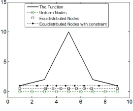
Figure 2: The comparison of three types of distribution for a test function
4 Numerical experiments
In this section, the algorithm is implemented on two time-dependent partial differential equations. The method is a combination of the algorithm which is introduced in 3.1 and Equidistribution algorithm (introduced in 3.3), re-garding the constraint (3). In fact, the e.d. algorithm is implemented in each step of time in meshless method of line to produce adaptive central nodes which satisfy the constraint (3).
Example 1. Consider the Burger equation
ut+u ux=υ uxx, (4)
on the interval [-1,1]. The exact solution is u(x, t) = 0.1eeaa++0.5eb+eebc+ec, where a = −(x+ 0.5 + 4.95t)/(20υ), b = −(x+ 0.5 + 0.75t)/(4υ), and
c=−(x+ 0.625)/(2υ). The initial conditionu(x,0) and the boundary con-ditions u(−1, t), u(1, t) are specified. By choosingυ = 0.0035,the equation is solved by uniform and adaptive nodes. Meshless method of line combined with adaptive algorithm is applied on equation (4). By choosing N center nodes{x1, x2, ..., xN} in the domain [-1,1], at a constant timet, the solution
u(x, t) can be expressed in RBF-approximation as follows
u(x, t) = N
∑
j=1
λjφ(rj) = Φt(r)λ. (5)
Collocating (5) by {x1, x2, ..., xN}, leads us to the following system of equa-tion
Aλ=u, (6)
whereu= [u(x1, t), u(x2, t), ..., u(xN, t)]. By substitutingλ=A−1uinto (5), we have
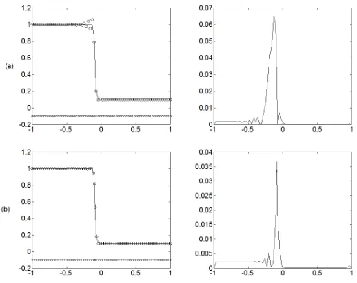
Figure 3: Plots of the approximate solution and absolute error of equation (4) at t=0.5 using 50 uniform nodes (a), adaptive nodes without constraint (b), and adaptive nodes with constraint (c)
where V(x) = Φt(x)A−1 = [V1(x), ..., VN(x)]. By substituting (7) into the Burger equation (4), and collocating the center nodesxi, we obtain
dui
dt +ui(Vx(xi)u) =υ (Vxx(xi)u), i= 1,2, ..., N.
This equation can be written as a system of ordinary differential equations as
du
dt =−u⊗(Vx(xi)u) +υ(Vxx(xi)u), (8)
where ⊗ denote component by component multiplication of two vectors. Equation (8), is rewritten as
du
Figure 4: Plots of the approximate solution and absolute error of equation (4) at t=1 using 70 uniform nodes (a), and adaptive nodes with constraint (b)
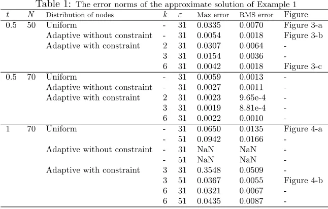
Table 1: The error norms of the approximate solution of Example 1
t N Distribution of nodes k ε Max error RMS error Figure
0.5 50 Uniform - 31 0.0335 0.0070 Figure 3-a
Adaptive without constraint - 31 0.0054 0.0018 Figure 3-b
Adaptive with constraint 2 31 0.0307 0.0064
-3 31 0.0154 0.0036
-6 31 0.0042 0.0018 Figure 3-c
0.5 70 Uniform - 31 0.0059 0.0013
-Adaptive without constraint - 31 0.0027 0.0011
-Adaptive with constraint 2 31 0.0023 9.65e-4
-3 31 0.0019 8.81e-4
-6 31 0.0022 0.0010
-1 70 Uniform - 31 0.0650 0.0135 Figure 4-a
- 51 0.0942 0.0166
-Adaptive without constraint - 31 NaN NaN
-- 51 NaN NaN
-Adaptive with constraint 3 31 0.3548 0.0509
-3 51 0.0367 0.0055 Figure 4-b
6 31 0.0321 0.0067
-6 51 0.0435 0.0087
-Example 2. Consider the KdV equation
ut+εu ux+µ uxxx= 0, (10)
withε= 6,andµ= 1. The initial condition is
u(x,0) = 2 sech2(x).
The exact solution is
u(x, t) = 2 sech2(x−4t).
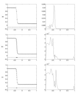
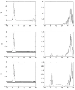
Figure 5: Plots of the approximate solution and absolute error of equation (10) at t=0.5 using 110 uniform nodes (a), adaptive nodes without constraint (b), and adaptive nodes with constraint (c)
Table 2: The error norms of the approximate solution of Example 2
t N Distribution of nodes k ε Max error RMS error Figure
0.5 110 Uniform - 0.8 0.1485 0.0389 Figure 5-a
Adaptive without constraint - 0.9 0.0460 0.0110 Figure 5-b Adaptive with constraint 2 1.2 0.0295 0.0069 Figure 5-c
3 1.2 0.0295 0.0069
-6 1.2 0.0295 0.0069
-0.5 150 Uniform - 0.8 0.0205 0.0065
-Adaptive without constraint - 0.8 0.0046 0.0014
-Adaptive with constraint 2 0.8 0.0033 0.0010
-3 0.8 0.0033 0.0010
-6 0.8 0.0033 0.0010
-1 150 Uniform - 0.8 0.0197 0.0094
-- 1.1 0.0074 0.0034
-Adaptive without constraint - 0.8 0.0045 0.0021
-- 1.1 0.0054 0.0025
-Adaptive with constraint 2 0.8 0.0033 0.0016
-2 1.1 0.0030 0.0014
-3 0.8 0.0033 0.0016
-5 Conclusion
In this paper, an Equidistribution algorithm has been applied to distribute the central nodes in adaptive modes to RBF methods. To have some smooth-ness properties, by the e.d. algorithm, the central nodes satisfying in a given constraint are obtained. This method was applied to two nonlinear time-dependent partial differential equations by MMOL. In numerical examples, the results obtained by uniform nodes, and adaptive nodes with, and with-out the constraint have been compared. The numerical results in Example 1, reveal that with adaptive nodes, a more accurate approximate solution has been obtained. Our numerical experience shows that, in this example, to achieve the accuracy as good as adaptive nodes, at least 150 uniform nodes must be applied. Also in Example 2, with 110 uniform nodes, the obtained results by adaptive nodes with constraint have better accuracy. With 150 center nodes a good accuracy has been obtained by three distributions. The numerical results in the examples illustrate the efficiency of adaptive nodes to solving some nonlinear PDEs with MMOL. The results show that apply-ing the adaptive central nodes is more accurate in the problems with speed gradient functions.
Acknowledgement The Authors are grateful to reviewers for their con-structive and helpful comments, which helped to improve the paper.
References
1. Behrens, J and Iske, A.Grid-free adaptive semi-Lagrangian advection us-ing radial basis functions, Computers & Mathematics with Applications, 43 (3–5) (2002) 319–327.
2. Belytschko, T., Krongauze, Y., Organ, D., Fleming, M. and Krysl, P Meshless methods: An overview and recent developments, Computer Methods in Applied Mechanics and Engineering, 139 (1996) 3–47 (spe-cial issue on Meshless Methods).
3. Bozzini, M., Lenarduzzi, L. and Schaback, R.Adaptive interpolation by scaled multiquadrics, Advances in Computational Mathematics, 16(4) (2002) 375-387.
4. Cao, W., Huang, W. and Russell, R. D.A study of monitor functions for two dimensional adaptive mesh generation, SIAM Journal on Scientific Computing, 20(6)(1999) 1978–1994.
6. Fasshauer, G. E. Mesh free Approximation Methods with MATLAB. World Scientific Co. Pte. Ltd., Singapore, 2007.
7. Ferreira, A. J. M., Kansa, E. J., Fasshauer, G. E. and Leitao, V. M. A. Progress on Meshless Methods, Computational Methods in Applied Sciences, Springer 2009.
8. Hon, Y. C.Multiquadric collocation method with adaptive technique for problems with boundary layer, International Journal of Applied Science and Computations, 6(3) (1999) 173–184.
9. Hon, Y. C., Chen, C. S. and Schaback, R. Scientific Computing with Radial Basis Functions. Draft version 0.0, Cambridge, 2003.
10. Hon, Y. C, Schaback, R. and Zhou, X. An adaptive greedy algorithm for solving large RBF collocation problems, Numerical Algorithms, 32(1) (2003)13–25.
11. Kansa, E. J. Multiquadrics-A scattered data approximation scheme with applications to computational fuid-dynamics-I surface approximations and partial derivative estimates, Computer and Mathematics with Ap-pllications, 19 (1990) 127–145.
12. Kansa, E. J. Multiquadrics-A scattered data approximation scheme with applications to computational fuid dynamics- II. Solution to parabolic, hyperbolic and elliptic partial differential equations, Computer and Math-ematics with Appllications, 19 (1990) 147–161.
13. Kautsky, J. and Nichols, N. K.Equi-distributing meshes with constraints, SIAM Journal on Scientific and Statistical Computing, 1(4) (1980) 449-511.
14. Quan, S. A meshless method of lines for the numerical solution of KdV equation using radial basis functions, Engineering Analysis with Bound-ary Elements, 33 (2009) 1171–1180.
15. Sanz-Serna, J. and Christie, I.A simple adaptive technique for nonlinear wave problems, Journal of Computational Physics, 67 (1986) 348-360.
16. Sarra, S. A. Adaptive radial basis function methods for time dependent partial differential equations, Applied Numerical Mathematics, 54 (1) (2005) 7994.
17. Schaback, R. and Wendland, H. Adaptive greedy techniques for ap-proximate solution of large RBF systems, Numerical Algorithms, 24(3) (2000)239–254.
ﯽﻤﺳﻮﻫ ﺪﻤﺤﻣ و رازآ ﯽﺑ ﺮﻔﻌﺟ
يدﺮﺑرﺎﮐ ﻲﺿﺎﻳر هوﺮﮔ ،ﻲﺿﺎﻳر مﻮﻠﻋ هﺪﮑﺸﻧاد ،نﻼﯿﮔ هﺎﮕﺸﻧاد
ﯽﻣ هدﺎﻔﺘﺳا ﯽﯾﺎﻀﻓ ﻪﻨﻣاد رد طﺎﻘﻧ ﻊﯾزﻮﺗ یاﺮﺑ رﺎﮔزﺎﺳ ﻪﮑﺒﺷ نوﺪﺑ ﻂﺧ شور ﮏﯾ زا ،ﻪﻟﺎﻘﻣ ﻦﯾا رد: هﺪﯿﮑﭼ ﯽﺻﺎﺧ یراﻮﻤﻫ ﻂﯾاﺮﺷ هﺪﺷ بﺎﺨﺘﻧا طﺎﻘﻧ ﻪﮐ ﺖﺳا مزﻻ یرﺎﯿﺴﺑ دراﻮﻣ رد ،ﻪﮑﺒﺷ نوﺪﺑ یﺎﻫ شور رد .دﻮﺷ ﯽﺳرﺮﺑ ﺎﻫ ﺖﯾدوﺪﺤﻣ ﻦﯾا زا ﯽﮑﯾ ،ﻪﻟﺎﻘﻣ ﻦﯾا رد .ﺪﻨﮐ قﺪﺻ ﯽﯾﺎﻫ ﺖﯾدوﺪﺤﻣ رد طﺎﻘﻧ ﻪﻋﻮﻤﺠﻣ و ﺪﻨﺷﺎﺑ ﻪﺘﺷاد ﯽﻃﺎﻘﻧ بﺎﺨﺘﻧا یاﺮﺑ ﺖﺳا ﻪﮑﺒﺷ نوﺪﺑ ﻂﺧ شور رد ﯽﻤﺘﯾرﻮﮕﻟا ندﺮﺑ رﺎﮐ ﻪﺑ ،ﻪﻌﻟﺎﻄﻣ ﻦﯾا زا فﺪﻫ .دﻮﺷ ﯽﻣ اﺮﻧآ ،ﺖﻗد ﺶﯾاﺰﻓا رد نآ ﯽﯾﺎﻧاﻮﺗ و ﻢﺘﯾرﻮﮕﻟا ﯽﯾارﺎﮐ نداد نﺎﺸﻧ یاﺮﺑ .ﺪﻨﻨﮐ قﺪﺻ ،ﺺﺨﺸﻣ ﯽﻄﯾاﺮﺷ رد ﻪﮐ .ﻢﯾﺮﺑ ﯽﻣ رﺎﮐ ﻪﺑ ﻪﻧﻮﻤﻧ لﺎﺜﻣ یداﺪﻌﺗ رد