*. Corresponding author address: Shahrood University of Technology, Shahrood
Tel.: +98 2332300240; fax: +98 2332300258, E-mail address: [email protected]
Design and Analysis of a Novel Tendon-less
Backbone Robot
M. Bamdad
a,*, A. Mardani
aa School of Mechanical and Mechatronics Engineering, Shahrood University, Shahrood, Iran, P.O. Box 3619995161
A R T I C L E I N F O A B S T R A C T
Article history: Received: July 4, 2015. Received in revised form: September 17, 2015. Accepted: September 27, 2015.
A new type of backbone robot is presented in this paper. The core idea is to use a cross shape mechanism with the principle of functioning of the scissors linkages, known as a pantograph. Although this continuum arm acts quite similar to tendon-driven robot, this manipulator does not include any tendon in its structure. This design does not suffer from the weaknesses of the continuum design such as low payload and coarse positioning accuracy. Kinematic model is developed and the equation of motion for this arm is derived by Lagrange's method. The work envelope and the occupied space investigation are supposed to be established on the comparison between tendon-based model as the common backbone models and our proposed idea. The results show the effectiveness of the backbone design.
Keywords: Mechanism design Continuum robot Tendon-based robot Kinematic analysis Dynamics
1. Introduction
The origin of continuum robotics is generally traced back to the creation of serpentine robots in the late 1960s [1]. These hyper-redundant robots employed a number of closely spaced joints to emulate the motion of the backbone of a snake. The ability of continuum backbones to bend at any point along their structure, together with their inherent compliance, offers continuum robots the potential to perform functions not feasible with conventional robots. They have been designed for three or two dimensional (3D-2D) manipulation tasks and shapes which are controlled by actuator inputs, such as tendon lengths, fluid pressures and both together in the pneumatic muscles, multi-backbone, multiple embedded tendons and concentric curved tubes.
The artificial muscles (pneumatic/hydraulic) use the combination of bending and force generation capabilities for continuum robots at a large scale,
meanwhile the extrinsic tendon-driven designs has the advantage of high force capability with light-weight structures [2].
Tendon-driven robots are divided to two main types: open ended and the endless robotic arm [3] Arms with one side tendon/one side spring are unable to hold large payloads and are only controllable from one side. It reserves power in the parts of its motion and releases it in the next cycles. Due to solve this problem, the coupled two side tendon driven manipulators were introduced [4].
Although the same number of tendons as actuators is required in tendon-driven manipulators, the branching tendon arrangement reduces the number of actuators while making lightweight robot. For simple adaptive grasping mechanisms, branching tendons have been suggested such as prosthetic hands in [5]. This design attempts to overcome the disturbance problems.
bandwidth. The authors in the prior research have investigated the fluctuation of tendon flexibility and the effect of tendons on controlling [6]. Not only the flexibility, but also the platform geometry is investigated in an optimization process for the branched tendon system [5].
Considering the influence of the overall tendon flexibility in a complicated control, Bamdad et al. propose a new mechanism not only reduces the length of tendons but also use a new two-bar mechanism in each bone to promote the platform [7]. The weaknesses of this multi-backbone design included low payload, poorly understood kinematics and dynamics, and coarse positioning accuracy [8]. While the constrained multi-backbone is connected within a single arc segment, 2-DOF bending actuation is achieved. Manipulators with constant length of curvature need to be armed by 2-curvature mechanism to follow 2D planar trajectories [9]. A continuum tendon-driven robot is essentially an infinite- DOF platform, controlled by applying forces or torques at periodic locations along the robot’s backbone [10]. This means that a specific set of tendon lengths does not imply a unique pose for the robot. Some researchers use a differential mechanism to manipulate two backbone robots as a 2-finger gripper by means of one actuator [10].
The piecewise constant-curvature assumption has the advantage of enabling kinematics to be decomposed into two mappings [11]. One is from joint or actuator space to configuration space parameters that describe constant-curvature arcs and the other is from this configuration space to task space, consisting of a space curve which describes position and orientation along the backbone.
In this paper a new type of backbone manipulator is proposed. The focus of this paper is on the multiple entities which are constrained and connected within a single arc segment to achieve 2-DOF bending actuation. Unlike many tendon-drive robot designs, which commonly utilize one tendon per joint, the idea includes a mechanism eliminating tendons and fabricating a trunk which can be extended in bending. A tendon-based continuum robot can transform to a circular shape by constant length and variable radius. In new proposed platform, the curvature has variable radius and length. It means that the structure is one curvature with 2DOFs.
Eliminating tendons increases rigidity and the motor can be set on each bone of manipulator. A tendon based continuum robot can transform to a circular shape by constant length and variable radius. New platform curvature has variable radius and length. It means that the structure is one curvature with 2DOFs. The kinematic and dynamic equations will be investigated while the constant curvature path is planned for end point movements.
A tendon-based robotic arm composed of cables and pulleys is assumed for a complete comparison study. It can be based on the use of evaluation criteria involving workspace [12]. To compute the possibility of the collision it is needed to consider the physical space occupied by the robot. The space in which a robot can operate is its work envelope, which encloses its workspace.
On the other hand, as shown by Salisbury and Craig [13], the condition number of Jacobian matrix of the manipulator can be defined as one kinematic index in workspace. It will give a measure of the accuracy of the Cartesian velocity of the end-effector and the static load acting on the end-effector.
The new platform advantages summarize in the items such as the vast work envelope, less occupied space by robot body during motion with the optimal dynamic behavior. The remainder of the paper considers the following aspects. The general concept of idea is described in the second section. The third stage is to express existent tendon-based models. Then the kinematic and dynamic equations of new platform will be obtained besides equations of existent model. The kinematic index is described. Finally, a simulation will be managed to show the ability of new platform in pure extension movement besides compounded extension and bending.
2. New design description
The ways to classify the designs are defined according to backbone characteristics and actuation strategies. Backbones may be either continuous (continuum robots) or discrete (hyper redundant robots), and may be fixed in length or can be extensible. This paper is accomplished by discrete actuators into the structure of the robot itself.
The continuum robots in this paper are most closely related to the concept of snake-like multi-backbone. These designs employ a series of several bending segments actuated by the backbone rods, tendons or linkages.
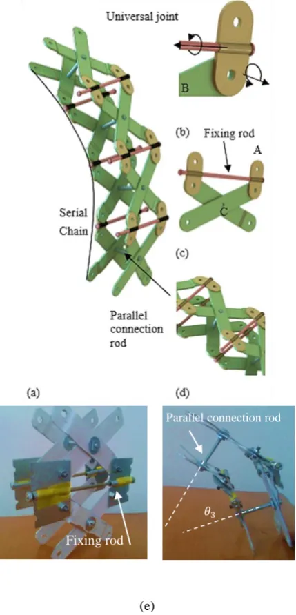
In this novel design, a scissors mechanism is utilized as segments in backbone. A series of crossed ternary links folds and extends. This criss-cross 'X' pattern is also seen in a pantograph, man-lifts and extensional gates. Figure 1 shows the platform. The whole shape of platform is illustrated in Figure 1.a within four bones.
illustrated in (c) is used to eliminate the rotation of universal joint about the axes “A” in (b).
Figure 1(c) explains the fixing way of universal joints in a cross mechanism. This connection allows to this cross bar to rotate around the other one by means of the universal joints.
The whole fabricated mechanism is composed of two serial chains connected together in a parallel form is depicted in (e).
(e)
Figure 1. (a) Complete platform, (b) Universal joint, (c) Cross unit, (d) Cross mechanism connection, (e) Fabricated sample
design.
Two serial chains are connected together in a parallel form which is illustrated in (a). Each serial chain is an independent mechanism actuated by an independent motor while from its topology, the mechanism consists of a serial chain of four-bar
linkages, and each four-bar in the chain shares two links with the previous four-bar in the backbone chain.
Figure 2 illustrates a complete kinematic chain of backbone including the linkage and actuation. The first motor is connected to a serial chain and second motor is located on the other chain which is connected to the bones. The cross mechanism of serial chain is actuated and pose independently. This difference provides the curvature forming. If the angle between two bars in a chain is similar to the bars of other chain, the manipulator will take the straight form. The cross segments keep the linkage shape close to the backbone. This means that the 2-DOF robotic arm can be easily controlled as a single DOF mechanism.
The backbone curve is the mechanism centerline or spine. The motor connection part is a fixture for motors to connect the rotors to a bone. The rotor of each motor is connected to one of the bars (bone) and the connection part is installed on the other bar of this bone.
This method of connection provides a condition to add motors on each arbitrarily cross mechanism. Moreover since the mechanism is not sensitive to the actuators connection location, more than two elements can be installed on each bone. For example, one or more than one spring can be connected to the bones to provide an active-passive mechanism.
All active or passive elements like motors or springs can be installed on each bone either on first bone, or nth-bone. In spite of almost platforms, this backbone is manipulated from the base. In addition, the most important advantage is that new platform is a 2-DOF structure just in one curvature.
Figure 2. Motors location
3. Tendon-based arm kinematics
The discrete tendon-driven backbone models can be categorized into two main types based on the using or Parallel connection rod
Fixing rod
not using the pulley. The second type is trunks which almost use tendon without pulley. Pulley-based manipulators are illustrated in Figure 3.
Tendon-based robot is an open ended manipulator. The central chamber length limits kinematics analysis. A comparison between cross backbone manipulator and existent tendon driven models will be managed consequently.
Figure 3. Tendon driven backbone manipulator armed by pulley [4]
The main parameters of the pulley-based manipulator are provided in Figure 4. It shows the motor and linkage, geometry parameter such as a the bone length,
𝐶𝐺𝑖, the center of the mass of link i as a segment of the
complete chain of the backbone. There are two actuators, the first one is connected to the first curve and the second one is connected to the second curve of linkage.
Figure 4. Kinematic of tendon-based backbone manipulator armed by pulley- kinematic parameters
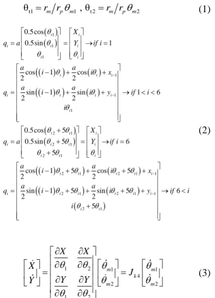
The relation between motor angle (𝜃𝑚1 and 𝜃𝑚2) and the angle of pulley (𝜃𝑡1 and 𝜃𝑡2) is described as Eq. 1.
The position and orientation of each bone is extracted as Eq.2.
The relation between end point position velocity and angular velocity of motors is provided in Jacobian matrix illustrated in Eq. 3. The inverse kinematic is provided in Eq. 4.
(1)
t1 1 t 2 2
θ rm rpm , θ rm rpm
(2)
1 1 1 1 1 1 2 1 2 1 2 1 0.5cos0.5sin 1
cos 1 cos
2 2
sin 1 sin 1 6
2 2
0.5cos 5 0.5sin 5
5
t i
i t i
t i
t t i
i t t i
t
t t i
i t t i
t t
X
q a Y if i
a a
i i x
a a
q i i y if i
i X
q a Y
2 1 2 1 1
2 1 2 1 1
2 1
6
cos 1 5 cos 5
2 2
sin 1 5 sin 5 6
2 2
5 i
t t t t i
i t t t t i
t t
if i
a a
i i x
a a
q i i y if i
i (3)
1 2 1 1
4 2 2 1 2 m m k m m X X X J Y Y Y
Pulley-based manipulator can't move freely due to some limits. If each curve of 2DOF manipulator bends more than a special angle (when 𝜃 approximates to
𝜃𝑚𝑎𝑥 value) collision happens. While 𝜃1 𝑚𝑎𝑥 and
𝜃2 𝑚𝑎𝑥 are the maximum possible value of motor
angles, Eq. 4 shows the collision condition and the final limit of rotation of each actuator is obtained.
(4) 1 1 2 2 2
5 2 5
5 2 2
5 max max
4. New platform kinematic
The main kinematic parameters of backbone are illustrated in Figure 6. The lengths of 'X' segments (each segment illustrated in Figure 1-c,d) L1, L3 and the total length of the manipulator curvature are
(6)
1 3
2
t
L
L
L
n
where n is the number of total bone and W is the length of the bar of each cross which is illustrated in Figure 6-(a). The curvature radius and the angle of each bone are obtained conditionally. Eq. 7 expresses the radius of curvature and 𝐶1 and 𝐶2 are conditional constants. Eq.
8 shows the angle of each bone.
(7) 2 1 2 1 1 2 1 2
1 3 1 2
3 1 1 2
1 3 1 2
cos 2 cos cos 2 2 cos 2 cos cos 2 2
1 , 0 0 , 1 ,
m
m m
m
m m
R C d
C d
L L C C
L L C C
L L C C
(8)
1 1 1 2
1 2
1 3 1 2
3 1 1 2
1 3 3
2 tan 2 tan
2 2
1 , 0 0 , 1 0
t
L L
C C
R R
L L C C
L L C C
L L
and the end point position 𝑋 and 𝑌 is:
(9)
1 cos sin t tX R n
Y R n
The position of each bone center
T i i i iq X Y
when i is the bone number is obtained based on the motors angles 𝜃𝑚1 and 𝜃𝑚2. The relation between curvature velocities and motor angles or chain angles is illustrated in Fig. 6 and could be calculated by Jacobian matrices.
(a)
(b)
Figure 5. Kinematic of cross backbone
(10)
1 1cos 1 cos
2 2
sin 1 sin 1
2 2
0.5cos
0.5sin 1
2
t t
t t i
t t
i t t i
t t t i t t L L
i i x
n n
L L
q i i y if i
n n
i
L
q if i
n
The Jacobian matrix of velocity can be extracted as the relation between motor velocity, curvature radius and curvature length, end point velocity. Using the relation of end point position velocity and motor velocity, the Jacobian of curvature length velocity, end point angle velocity 𝜃𝑒̇ and motor rates is obtained in Eq. 13.
(11)
1 2 1 1
1 2 2 1 2 t t t m m k m m L L R L J R R (12)
1 2 1 1
2 2 2 1 2 m m k m m X X X J Y Y Y (13) 1 3 2 t m k e m L J (14)
1 1 1
1
1 2 3
2
t m
k k k
e m
t X L
J J R L J Y
Inverse kinematic is defined in Eq. 11. If the aim was pure bending, the Eq. 13 is required. If manipulator was assumed to follow end point path, Eq. 12 is required. If compounded mission or pure extension was required, Eq. 14 is used. The end point velocity is derived from motor angles by 𝐽𝑘2 in Eq. 16. The closed form 𝐽𝑘1 is
5. Condition number
The condition number of Jacobian matrix of the manipulator can be defined as one kinematic index in workspace. It is possible to compare error propagation with different manipulator configurations if condition number of T
J was investigated. One of the anticipated
uses of this hand is in force-controlled tasks, and the location of most accurate operation points is a useful design consideration. The transpose of the Jacobian matrix, J, is a linear transform from joint torques to forces, exerted at the end point. If we consider error propagation in linear systems [13], we note that the relative error of end point force F F/ is bounded by the product of the condition number of the Jacobian transpose matrix and the relative error in joint torque
. /
c where c is condition number. The condition number is limited between 1 and infinity. One shows the best response of condition number because by a constant error of motor torques the end point force error takes minimum value. A new parameter can be defined
as 1
Dc which is limited between 0 (the worst) and 1 (the best).
6. Inverse kinematic and Dynamics
The resolved motion rate control is provided by the inverse kinematic equation and Jacobian 1
2
k
J maps
the end point velocity to motor displacement.
The inertia of manipulator is assumed much smaller than the external force and mass of robot. The dynamic equations are developed for a 2-DOFs model driven by two motors. Typical dynamic equation is extracted by Lagrange’s method. Inertia of link is assumed to be zero. H is inertia matrix and G, C are gravity effect and non-linear terms.
(15) 1 2
[ ]T
m m HGC
The motor velocity and acceleration is utilized to find motor torques which are expressed as 𝜏𝜃1and 𝜏𝜃2.
(16) 1
1 2 1 2 1
1 2
2 2 2
2
1
2
k
m k m k m
m m
m m
m m m
X J J
J Y
(17)
1 1
2 2
m m
m m
H G C
7. Simulation
The simulation shows the proposed linkage mechanism presented in this paper attempts to overcome the kinematic and dynamic limitations. Kinematic and dynamic equations successfully predict all of the major qualitative and quantitative features of the backbone arm movements. The assumed value of main properties is provided in Table. 1.
The aim of simulation of this paper is to compare existent tendon-based model to our new platform. Moreover special ability to provide the pure extension movement is demonstrated.
The tendon-based backbone design is based on the behavior raised from biomechanical constraints, anatomy of the human hand. The mechanism is inclusive of cables, pulleys, guides to achieve under-actuation and coupling between the bones.
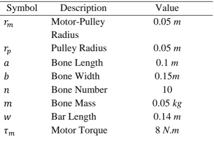
Table 1. Numerical properties of the simulation models
Symbol Description Value
𝑟𝑚 Motor-Pulley
Radius
0.05 m
𝑟𝑝 Pulley Radius 0.05 m
𝑎 Bone Length 0.1 m
𝑏 Bone Width 0.15m
𝑛 Bone Number 10
𝑚 Bone Mass 0.05 kg
𝑤 Bar Length 0.14 m
𝜏𝑚 Motor Torque 8 N.m
7.1.Work Envelope
While the workspace of the robot defines end-effector poses that it can achieve to task accomplishment. The work envelope include the volume of the robot itself occupies as it moves. The work envelope comparison between a tendon-based model (Fig. 5) and the new mechanism are presented in Figure 7.
The swarm of points as the red stars denotes the possible area of the work envelope of continuum models.
Depending on the motion direction, the robot body will span a certain longitudinal and a certain lateral space related to the robot shape. We call the space containing obstacles the occupied space.
About Y axis, the access length is 0.2 m more than others. Other important matter is to access to near point to the base of robot by means of end point of manipulators. This access is provided in work envelope of cross manipulator especially in 𝑋 > 0 Points. Total area of cross work envelope is more than others. To compute the possibility of the collision it is needed to consider the physical space occupied by the robot. Reaching to the work envelope boundaries is one of the most important limitations in kinematic investigations but another important matter must be considered is the occupied area during motions. Occupied area is the part of space that is occupied by means of all part of body during motion.
Figure 6. Work envelope of tendon-based model
Figure 7. Work envelope of ‘X’ platform
The physical size of this envelope within the motion is investigated. The difference of new robot and tendon-based manipulators will be clearly depicted when manipulators are forced to follow horizontal path:
(18)
1 0.25 1 cos
0 t X
Y
where it is a time-dependent horizontal path and the simulation time is π s. Taking into account the space occupied by the body of robot, Figure 8 shows obviously this fact that new cross platform move on a line and the occupied space of movement is ignorable but tendon-based platform move in the workspace while the robot body occupy considerable space.
(a)
(b)
Figure 8. Horizontal path (a) Tendon-based (b) New platform
7.2.Condition number
Robots attempt to move into the work envelope which is resolved by joint motion. To obtain a general view of a robot moving into an occupied space, an index can be chosen. New structure has no more ability in movement is the far regions from center of the fixed coordinate in [0 0]. On the other hand, in the points of the work envelope that tendon based manipulators have no access, the movement ability of new platform is more than other points. This point is illustrated by magenta color.
-0.6 -0.4 -0.2 0 0.2 0.4 0.6 0.8 1
-1 -0.8 -0.6 -0.4 -0.2 0 0.2 0.4 0.6 0.8 1
X(m)
Y
(m
)
-0.4 -0.2 0 0.2 0.4 0.6 0.8 1 1.2 1.4 -1
-0.8 -0.6 -0.4 -0.2 0 0.2 0.4 0.6 0.8 1
X(m)
Y
(m
)
0 0.2 0.4 0.6 0.8 1
-0.5 -0.4 -0.3 -0.2 -0.1 0 0.1 0.2 0.3 0.4 0.5
X(m)
Y
(m
)
Work space
-0.2 0 0.2 0.4 0.6 0.8 1 1.2 -1
-0.8 -0.6 -0.4 -0.2 0 0.2 0.4 0.6 0.8 1
X(m)
Y
(m
7.1.Dynamic simulation
Fig. 11 shows a line in X-Y plane as a path for the end point of continuum arm. The inverse dynamic and kinematic is simulated for both models.
(19)
1 0.25 1 cos
, 0 0.5sin
t X
t
Y t
(a)
(b)
Figure 9. D plots (a) Tendon-based (b) New platform. The colors mentioned consequently denotes the value Black, D<0.001-blue, 0.001<D<0.01, -green, 0.01<D<0.1-magenta,
0.1<D<0.3-cyan, 0.3<D<0.5-yellow, 0.5<D<0.8-red, 0.8<D<1
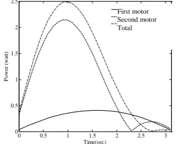
As it is shown in Figure 10, arm gets close to the boundaries of the work envelope. These constraints arise from limited joint travel range. Figure 11 plots the angular displacement, torques and power of two motors. According to Figure 11.a , the angle of motors gets close to each other and it means the platform performs near to singular point.
Figure 10. Trajectory of tendon-based manipulator
(a)
(b)
(c)
Figure 11. Pulley-Motor result. (a) Angular displacement (b) Torques (c) Power
-0.4 -0.2 0 0.2 0.4 0.6 0.8 1 1.2 -1
-0.5 0 0.5 1
X(m)
Y
(m
)
-0.4 -0.2 0 0.2 0.4 0.6 0.8 1 1.2 -1
-0.5 0 0.5 1
X(m)
Y
(m
)
0 0.1 0.2 0.3 0.4 0.5 0.6 0.7 0.8 0.9 1 -0.4
-0.3 -0.2 -0.1 0 0.1 0.2 0.3 0.4 0.5 0.6
X(m)
Y
(m
)
0 0.5 1 1.5 2 2.5 3
-0.1 0 0.1 0.2 0.3 0.4 0.5 0.6 0.7
Time(sec)
A
n
g
u
la
r
d
is
p
la
ce
m
en
t
(R
ad
)
Second motor First motor
0 0.5 1 1.5 2 2.5 3
0 2 4 6 8 10 12 14
Time (sec)
T
o
rq
u
e(
N
.m
)
First motor Second motor
0 0.5 1 1.5 2 2.5 3 3.5 0
0.2 0.4 0.6 0.8 1 1.2 1.4 1.6
Time (sec)
P
o
w
er
(
w
at
t)
Figure 12 shows the same path for ‘X’ mechanism. Robot work envelope layouts must include considerations of regions of limited accessibility where the structure and the mechanical linkage may experience movement limitations. The cross backbone manipulator has more distance to the boundaries of the work envelope. Moreover, the vast work envelope of provides a wide range of possible path planning for ‘X’ mechanism.
Figure 13-a, shows the angular displacement of each motor. The motor torques and power are illustrated in Figure 13-b, c. Generally, Fig. 13 shows more smooth plots compare to Fig. 12. It demonstrates an improvement on the dynamic behavior.
Figure 12. Trajectory of cross manipulator
Figure 13. ‘X’-Motor result. (a) Angular displacement (b) Torques (c) Power
8. Mechanism Disadvantages
In spite of all design benefits, some important challengeable maters should be considered such as: friction issue, weight of system, the contact of elements, the clearance and the number of elements. These items could play a big role in the new platform disadvantages. The most destructive one is the friction between the parts.
Indeed due to the number of parts and the required accuracy of each hole, pine and link, eliminating the clearance becomes harder than other existent model. Moreover the quite large number of parts makes the process of design, optimization and production, harder and may take a lot of time to obtain an acceptable model and simulation.
9. Conclusion
The paper describes design and modeling of a new tendon-less continuous backbone robotic. Architectures form the backbone of complete robotic system and two motors for the motion control. The results show that the main goals to eliminate tendons and obtaining a 2-DOFs manipulator by one curvature have been satisfied. The work envelope of new model is more than other existent models and approximately all points in the border of work envelope are available. The condition number shows that new platform has less error of the force of end point as compared to tendon-based models.
-0.4 -0.2 0 0.2 0.4 0.6 0.8 1 1.2
-0.2 0 0.2 0.4 0.6 0.8
X(m)
Y
(m
)
0 0.5 1 1.5 2 2.5 3
1.5 1.6 1.7 1.8 1.9 2 2.1 2.2
Time (sec)
A
n
g
u
la
r
d
is
p
la
ce
m
en
t
(R
ad
)
First motor Second motor
0 0.5 1 1.5 2 2.5 3
-10 -8 -6 -4 -2 0 2 4 6 8 10
Time(sec)
T
o
rq
u
e
(N
.m
)
First motor Second motor
0 0.5 1 1.5 2 2.5 3
0 0.5 1 1.5 2 2.5
Time(sec)
P
o
w
er
(
w
at
t)
References
[1] M. E. Rosheim, “Robot evolution: the development of anthrobotics”, John Wiley & Sons, (1994).
[2] M. H. Korayem, M. Bamdad and M. Saadat, “Workspace analysis of cable-suspended robots with elastic cable”, IEEE International Conference, (2007), pp. 1942-1947.
[3] J. J. Lee and Y. H. Lee, “Dynamic analysis of
tendon driven robotic mechanisms”, Journal of Robotic
Systems, Vol. 20(5), (2003), pp. 229-238.
[4] S. Hirose, and S. Ma, “Coupled tendon-driven
multijoint manipulator”, Robotics and Automation Proceedings, IEEE International Conference, (1991). [5] M. Bamdad, and A. Mardany, “Motion analysis of continuum robots structures with cable actuation”, Modares Mechanical Engineering, Vol. 14(14), (2015).
[6] M. Bamdad and A. Mardany, “Mechatronics
modeling of a branching tendon-driven robot”, Robotics and Mechatronics (ICRoM), Second RSI/ISM International Conference, (2014), pp. 522-527
[7] M. Bamdad and A. Mardany, “Design and analysis of a novel cable-driven backbone for continuum
robots”, Modares Mechanical Engineering, Vol. 15(3)
(2015).
[8] W. McMahan, J. Bryan, I. Walker, V. Chitrakaran,
A. Seshadri, and Darren Dawson, “Robotic
manipulators inspired by cephalopod limbs”,
Proceedings of the Canadian Engineering Education Association, (2011).
[9] I. Gravagne, and I. D. Walker, “Uniform regulation of a multi-section continuum manipulator”, Robotics
and Automation Proceedings, ICRA'02, IEEE
International Conference, (2002).
[10] L. Birglen, and C. M. Gosselin, “Force analysis of connected differential mechanisms: application to
grasping”, The International Journal of Robotics
Research, Vol. 25(10), (2006), pp. 1033-1046.
[11] B. Jones, and I. D. Walker, “Kinematics for
multisection continuum robots,” Robotics, IEEE
Transactions on 22, (1), (2006), pp. 43-55.
[12] J. Angeles, and F. C. Park, “Performance evaluation and design criteria”, Springer Handbook of Robotics, Springer, (2008), pp. 229-244.
[13] J. K. Salisbury, and J. J. Craig, “Articulated hands
force control and kinematic issues”, The International
Journal of Robotics Research, Vol. 1(1), (1982), pp. 4-17.
Biography
Mahdi Bamdad received
his BS, MS, and PhD degrees all in Mechanical Engineering in 2004, 2006, and 2010, respectively. Currently, he is an assistant professor with Shahrood University of Technology. He as a head of mechatronics group developed course curricula with proposed syllabus for mechatronics and programme at School of Mechanical and Mechatronics Engineering. He teaches courses in the areas of robotics, dynamics, automation, analysis, and synthesis of mechanisms. His research interests are in the areas of dynamics modeling, mechanisms design, optimization of robotic and mechatronic systems. He has published more than 60 articles in national and international journals and conference proceedings.
Appendix
Appendix. A
𝐽𝑘1= [−
sin (θ1
2 ) 5 −
sin (θ2
2 ) 5 𝑈0 𝑈1+ 𝑈2
] , 𝐽𝑘2
= [
U3
U4+
U5U6
U7 −
U8
U9−
U10
U11−
U12U13
U14
U15
U16+
U17U18
U19 −
U20U21
U22 −
U23
U24−
U25
U26]
(P-1)
𝑈0= −
3cos (θ2
2 ) sin (θ2 )1 20000 (cos (
θ1
2 ) 10 −
cos (θ2
2 ) 10 )
2
(P-2)
𝑈1=
0.0015 𝑠𝑖𝑛(0.5 𝜃2)
0.1𝑐𝑜𝑠(0.5 𝜃1) − 0.1 𝑐𝑜𝑠(0.5 𝜃1) (P-3)
𝑈2=
1.5 104𝑐𝑜𝑠(0.5𝜃
2)𝑠𝑖𝑛(0.5𝜃2)
(0.1 𝑐𝑜𝑠(0.5𝜃1) − 0.1 𝑐𝑜𝑠(0.5𝜃2))
2 (P-4)
U3= 3cos (
θ2
2) sin ( θ1
2) (cos(𝑌1) − 1)
𝑌1=
800cos (θ1
2 ) ( cos (θ1
2 ) 10 −
cos (θ2
2 ) 10 ) 3cos (θ2
2 )
(P-5)
U4= 200 (cos (
θ1
2) − cos ( θ2
2))
2
= U11= U16 (P-6)
U5= 3sin(𝑌2) = U12
𝑦2=
800cos (θ1
2 ) ( cos (θ1
2 ) 10 −
cos (θ2
2 ) 10 ) 3cos (θ2
2 )
(P-7)
U6= cos (
θ2
2) (Y3+ Y4)
𝑌3=
40cos (θ1
2 ) sin (θ2 )1 3cos (θ2
2 )
𝑌4=
400sin (θ1
2 ) ( cos (θ1
2 ) 10 −
cos (θ2
2 ) 10 ) 3cos (θ2
2 )
(P-8)
U7= 100(𝐷1) = U19= U14= 0.5 U9
𝐷1= cos (
θ1
2) − cos ( θ2
2)
(P-9)
U8= 3sin (
θ2
2) (cos(𝑌5) − 1)
𝑌5=
800cos (θ1
2 ) ( cos (θ1
2 ) 10 −
cos (θ2
2 ) 10 ) 3cos (θ2
2 )
(P-10)
U10= 3cos (
θ2
2) sin ( θ2
2) (cos(𝑋1) − 1)
𝑋1=
800cos (θ2
2 ) ( cos (θ1
2 ) 10 −
cos (θ2
2 ) 10 ) 3cos (θ2
2 )
(P-11)
U13= cos (
θ2
2) ( 40cos (θ1
2 ) sin (θ2 )2 3cos (θ2
2 )
+ 𝑋2)
𝑋2=
400cos (θ2
2 ) sin (θ2 ) (2 cos (θ1
2 ) 10 −
cos (θ2
2 ) 10 ) 3cos (θ2
2 )
2
(P-12)
U15= 3sin(𝑋3)cos (
θ2
2) sin ( θ1
2) (P-13)
𝑋3=
800cos (θ1
2 ) ( cos (θ1
2 ) 10 −
cos (θ2
2 ) 10 ) 3cos (θ2
2 ) U17= 3cos(𝑋4)cos (
θ1
2)
𝑋4=
800cos (θ1
2 ) ( cos (θ1
2 ) 10 −
cos (θ1
2 ) 10 ) 3cos (θ1
2 )
(P-14)
U18
= (
𝑋5+
400sin (θ1
2 ) ( cos (θ1
2 ) 10 −
cos (θ2
2 ) 10 ) 3cos (θ2
2 )
) 𝑋5=
40cos (θ1
2 ) sin (θ2 )1 3cos (θ2
2 )
(P-15)
U20= 3cos(𝑋6)cos (
θ2
2)
𝑋6=
800cos (θ1
2 ) ( cos (θ1
2 ) 10 −
cos (θ2
2 ) 10 ) 3cos (θ2
2 )
(P-16)
U21
=40cos ( θ1
2 ) sin (θ2 )1 3cos (t22 )
+
400cos (θ1
2 ) sin (θ2 ) (2 cos (θ1
2 ) 10 −
cos (θ2
2 ) 10 ) 3cos (θ2
2 )
2
(P-17)
U22= 1000 (
cos (θ1
2 ) 10 −
cos (θ2
2 )
10 ) (P-18)
U23= 3sin(𝑋7)sin (
θ2
2)
𝑋7=
800cos (θ1
2 ) ( cos (θ1
2 ) 10 −
cos (θ2
2 ) 10 ) 3cos (θ2
2 )
(P-19)
U24= 2000 (
cos (θ1
2 ) 10 −
cos (θ2
2 )
10 ) (P-20)
U25= 3sin(𝑋8)cos (
θ2
2) sin ( θ2
2)
𝑋8=
800 ∗ cos (θ1
2 ) ( cos (θ1
2 ) 10 −
cos (θ2
2 ) 10 ) 3cos (θ2
2 )
(P-21)
U26= 20000 (
cos (θ1
2 ) 10 −
cos (θ2
2 ) 10 )
2