Volume 5 - Article 1 | Pages 1–22

in the population sciences published by the Max Planck Institute for Demographic Research Doberaner Strasse 114 · D-18057 Rostock · GERMANY www.demographic-research.org

DEMOGRAPHIC RESEARCH

VOLUME 5, ARTICLE 1, PAGES 1-22

PUBLISHED 19 SEPTEMBER 2001

www.demographic-research.org/Volumes/Vol5/1/

DOI: 10.4054/DemRes.2001.5.1

Expanding an abridged life table

Anastasia Kostaki

Vangelis Panousis

1. Introduction 2

2. Expanding methodology 3

3. Comparisons 9

4. Concluding remarks 11

Expanding an abridged life table

Anastasia Kostaki 1 Vangelis Panousis 2

Abstract

A question of interest in the demographic and actuarial fields is the estimation of the age-specific mortality pattern when data are given in age groups. Data can be provided in such a form usually because of systematic fluctuations caused by age heaping. This is a phenomenon usual to vital registrations related to age misstatements, usually preferences of ages ending in multiples five. Several techniques for expanding an abridged life table to a complete one are proposed in the literature. Although many of these techniques are considered accurate and are more or less extensively used, they have never been simultaneously evaluated. This work provides a critical presentation, an evaluation and a comparison of the performance of these techniques. For that purpose, we consider empirical data sets for several populations with reliable analytical documentation. Departing from the complete sets of qx-values, we form the abridged

ones. Then we apply each one of the expanding techniques considered to these abridged data sets and finally we compare the results with the corresponding complete empirical values.

1 _{Department of Statistics, Athens University of Economics and Business, 76 Patision St., Athens 10434,}

Greece. Email: kostaki@ aueb.gr

2

Department of Statistics, Athens University of Economics and Business, 76 Patision St., Athens 10434,

1. Introduction

Mortality and fertility form the two general causes of the physical notion of a human population. Both causes are object of great attention and analysis by demographers. A demographer constructs a life table in order to describe the survivorship of a population as subjected to the risk of death. Such a table describes the effect of mortality. An abridged life table presents the mortality pattern by age groups. The problem of estimating a complete life table, when the data are provided in age intervals has been extensively discussed in demographic, biostatistical, as well as actuarial literature. The main reason for providing data in an abridged form are related to the phenomenon of age heaping, caused by age misstatements in data registration. Another typical reason is the unstable documentation of vital statistics based on insufficiently small samples. The most typical age-misstatements is the preference of ages ending in multiples of five. Such misstatements cause the appearance of age heaps. An example of such age preference in empirical data is illustrated below. The data are the observed number of deaths of the Greek female population in 1960.

The common approach to overcome this source of systematic errors adopted by the various statistical offices is to group the data in five-year age groups having the motivation that these over- and understatements which affect the age-specific data sets will efface each other into the five-year age group.

The Mortality of the 1960 Greek Female Population

age x

81 77 73 69 65 61 57 53 49 45

deaths dx

However, for several reasons, there is a need for reliable estimations of mortality rates specific by age. Several methods have been suggested in the literature for reproducing the age-specific mortality pattern. Techniques that utilize some general interpolation formula as King (1914), Beers (1944) have been extensively used previously. An interpolation method that is still very actual is the six-term Lagrangean formula to be applied to the existed in an abridged life table, lx values. This method is

presented in Abramowitz and Stegun (1965) and it forms the only expansion technique proposed in standard textbooks as Elandt-Johnson and Johnson (1980), and Namboodiri (1991). J.Pollard (1989) presents a relatively new one that requires five-year age grouping. Another technique for expanding an abridged life table has developed by Kostaki (1987) and also developed independently within the MORTPAK and MORTPAK-LITE software packages published by the United Nations (1988a, 1988b). For the application of this technique a parametric model of human mortality is required. In Kostaki (1987), as well as in the MORTPAK package the eight-parametric model of Heligman and Pollard (1980) is used. Additionally, in Kostaki (1991) a final adjustment to the results of this expanding technique is also developed. Some years later, Kostaki (2000) presented a non-parametric technique, in the sense that it does not require the use of a parametric model. The new method relates the target abridged life table with an existed complete one that is utilized as a standard. Interpolation via splines is a case of an osculatory interpolation that has lately received great attention. Great literature refer to splines, as tools for expanding an abridged life table (see e.g. Hsieh, 1991, McNeil, et. al., 1977, Wegman and Wright, 1983).

Although most of these techniques are considered accurate and are extensively used, their performance has never been compared and simultaneously evaluated. This paper provides an evaluation and a comparison of the performance of the various techniques. For that purpose, we consider empirical data sets for several populations with reliable analytical documentation. Departing from the complete set of qx-values of

each population, we form the corresponding abridged ones. We then apply each one of the expanding techniques considered to the abridged data sets and finally we compare the resulting age-specific probabilities with the age-specific empirical values.

Next section is devoted to a presentation of the different techniques. Then in Section 3 we present and evaluate the results of our calculations while in the last section some concluding remarks are provided.

2. Expanding methodology

1980) is the use of the six-term Lagrangean interpolation formula on the existing in the abridged life table,

l

_x-values. This formula expresses each non-tabulated value

l

_x as a linear combination of six particular polynomials in x, each of degree five,

∑∏

=

∏

≠ ≠

−

−

=

6 1 i i i j j i i j j

)

x

(

l

)

x

x

(

)

x

x

(

)

x

(

l

(1)

where x1, x2, …, x6 are the tabular ages nearest to x.

Let us now turn to spline interpolation. There is some enormous literature on splines, most of it concerning their numerical analytic properties (see e.g. DeBoor, 1978, Greville, 1969, Tyrtyshnikov, 1997), rather than their statistical properties (see e.g. Green, Silverman, 1995, McNeil, et.al., 1977, Härdle, 1992 or, Wahba, 1975). Special interest has been shown lately to such osculatory polynomials on the course of Demography.

A spline, symbolized as S, is a function derived after joining a sequence of polynomial arcs. Suppose that

a

=

x

o

<

x

1

<

...

<

x

n+1

=

b

, then a spline

S

of

degree

k

defined on the interval [a, b] with internal “ knots ”

x

1

,...,

x

_n is a function

such that, if

0

≤

i

≤

n

and

x

_i

≤

x

≤

x

_i+1, then

S

(

x

)

=

p

i

(

x

)

where

p

i

(

x

)

is a polynomial in

x

of degree not greater than

k

. The polynomial arcs meet at pivotal values are called knots. Splines are related to the roughness penalty approach of Green and Silverman (1995). The roughness penalty approach for curve estimation is stated as follows.

Given any twice - differentiable function S defined on [a,b], and a smoothing parameter ?, define the modified sum of squares,

∑

−

+

λ

∫

′′

=

= n 1 i b a 2 2 i i function penalty roughness

dx

))

x

(

S

(

))

t

(

S

Y

(

)

S

(

L

4

4 3

4

4 2

1

The penalized least squares estimator

Sˆ

is defined to be the minimizer of the functional

)

S

(

S:









→

∞

→

λ

.

a

to

tend

will

S

then

,

0

.

a

to

tend

will

S

then

,

if

curve

ing

interpolat

smooth

model

regression

linear

A simple representation of the interpolating spline of degree k can be written in the following way.

∑

∑

= + =

−

+

=

n i k i i k j j

j

x

c

x

x

d

x

S

1 0

)

(

)

(

where

).

0

)

((

otherwise

zero

and

0

)

(

if

,

)

(

x

−

x

i ₊

=

x

−

x

i

x

−

x

i

≥

x

−

x

i

<

The x’s into the formula are the data points where the polynomials meet (i.e. the knots) while d’s and c’s are parameters. They are all of number n+m+1. For k=3 one can get the cubic spline interpolant. Two cases of the cubic spline are the most famous:

The Natural cubic spline

Among the set of all smooth curves S in

S

[

a

,

b

]

interpolating the points

(

x

_i

,

z

_i

)

, the one minimizing

∫

S

"

2 of L(S) is a natural cubic spline with knots

x

_i. Furthermore provided

n

≥

2

there is exactly one such natural spline interpolant. This is introduced by the uniqueness theorem that says that supposing that

n

≥

2

and

x

₁

<

...

<

x

_n, given any values

z

₁

,

z

₂

,...,

z

_n, there is a unique natural cubic spline S with knots at the points

x

_i satisfying,

n

,...

1

i

for

,

z

)

x

(

S

i

=

i

=

The Complete cubic spline

same definition of the natural one but with no natural conditions applied to the ends of the data. Hsieh (1991) gives further details for the end conditions.

McNeil, et.al. (1977), present the first analytic application of spline interpolation to demographic data. They present and adopt the cubic spline solution to a demographic interpolation problem concerning fertility for Italian women of 1955. Such an application has to deal with rates that begin by age x=15, and not by the age zero which is the case when we have to interpolate the

l

_x- values of a life table.

Benjamin and Pollard (1980) present in detail spline smoothing and interpolation in mortality analysis. By adopting the natural cubic spline, they produce the graduated mortality rates for a certain life table example. McCutcheon (1981), deals with certain aspects of splines at a greater length. Applications are concerned with the construction of some U.K. National Life Tables. Details of that may also be found in the work of McCutcheon and Eilbeck (1977). An interesting survey article on splines in Statistics is the one of Wegman, and Wright (1983), that attempts to synthesize a variety of works on splines in Statistics.

Later developments of the cubic spline mostly deal with fertility data. Nanjo (1986, 1987) describes the use of rational spline functions, which include cubic spline as a special case in obtaining data for single years of age for births given by five-year age groups of mothers. Barkalov (1988) also describes the use of rational splines for demographic data interpolation. Bergström, and Lamm (1989) apply cubic spline interpolation in order to recover event histories. The method is used in order to adjust the U.S. age at marriage schedules explaining a substantial part of the discrepancy in the 1960 and 1970 censuses.

Hsieh (1991a,b) presents interesting applications of splines on Canadian data. The author develops a set of new life table functions, which also includes in the formulation of what he calls complete cubic spline interpolation method.

Applications concerning splines in Demography also appear later in the literature, all of them concerning the smoothing spline case (see, e.g., Biller, and Färhmeir, 1997, Green, and Silverman, 1995, Renshaw 1995). Finally, Haberman & Rensaw (1999) present the more recent application of spline functions in the course of Demography by developing a simple graphical tool for the comparison of two mortality experiences. Readers interested to study the subject of spline functions further, may consult, Greville (1969), DeBoor (1978), Härdle (1992), Green and Silverman (1995).

q

q

A

D

E

x F

GH

x

x

x BC x

1

2

−

=

+

+

−

+

( )

exp(

(ln( / )) )

(2)

Using the notation C for the parameters of the model (2) and the notation F(x;C) for the right hand side of (2), we get

q

F x C

F x C

x

=

+

=

( ; )

( ; )

1

(3)

=

G x C

( ; )

say, and hence the relation

n x x i

i n

q

= −

−

q

₊

= −

∏

1

1

0 1

(

)

implies the model

n x i n

q

= −

−

G x

+

i C

= −

∏

1

1

0 1

(

(

; )

=

_n

G x C

( ; )

say, the later being an explicit but complicated function of C, x, and n.

Thus given the values of nqx of the abridged life table one provides estimates of C

minimizing

(

n

( ; )

)

n x x

G x C

q

∑

−

1

2 (4)

where the summation is over all relevant values of x. Then inserting this C into (3) estimates of the one-year qx-values are produced.

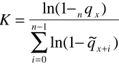
K

q

q

n x

x i i

n

=

−

−

₊

= −

∑

ln(

)

ln(

~

)

1

1

0 1

and the adjustment of the results

q

~

x through calculation of

~

_{′ = − −}

₍

_{~ )}

q

_x

1 1

q

_x K .

This final adjustment produces results

(~ )

q

_x

′

fulfilling the property:

1

1

1 1

−

− ′ =

= −

+

∏

i n

x i n x

q

q

(

~

)

.

Kostaki (2000) presents a simple non-parametric expanding technique. According to that, the abridged nqx-values to be expanded are related to the one-year probabilities

qx(S) of another complete life table which is solely utilized as a standard.

Under the assumption that the force of mortality, µ(x), underlying our abridged life table is, in each n-year age interval [x, x+n), a constant multiple of the one underlying the standard life table in the same age interval, µ(S)(x), i.e.,

µ

( )

x

=

_n

K

_x

*

µ

( )S

( )

x

,

the one-year probabilities qx+i, i= 0,1,..., n-1, in each n-year interval are equal to

1 1

− −

(

q

( )_{x i+}S

)

nKx ₍₅₎

where,

n x

n x

x i S i

n

K

q

q

=

−

−

₊

= −

∑

ln(

)

ln(

( )

)

1

1

0

1 (6)

Thus, having the values of nqx of the abridged life table, as well as, the set of

calculates the values of nKx using (6) and then inserting these values in (5) produces

estimates for the one-year probabilities qx underlying the original abridged life table.

3. Comparisons

In order to evaluate and compare the performance of the various methods described above, we use empirical data from several populations and several time periods. We have the empirical

q

_x - values which we initially abridge in wider age intervals for the ages 0, 1-4, 5-9... e.t.c. Then we apply each one of the presented expanding methods using these abridged datasets. At a final step, we compare the resulting complete sets with the corresponding complete empirical ones.

For the purpose of the evaluation and comparison of the performance of the different techniques used, we provide graphical representations of the results and we calculate the values of two different criteria. These are the sum of squares of the absolute and the relative deviations between the resulting and the empirical

q

_x - values,

2

)

ˆ

(

x

x

x

q

q

∑

−

(7)

and

2

)

1

ˆ

(

−

∑

x x

x

q

q

(8)

The rationale behind the choice of criteria (7) and (8) is that they complete each other since their values are indicative for the performance of a technique at the higher respectively the earlier part of the total age interval.

The interpolating polynomial spline applied on the

l

_x - values of the abridged life table was obtained in S-plus (see Chambers and Hastie, 1992).

converge and stopped. In cases where the empirical evidence was very sparse MORTPAK did not suggested adequate initial values. In such cases we obtained initial parameter values using a stepwise estimation procedure proposed in Kostaki (1992)b. In order to obtain estimates for the standard errors of the parameters of HP8, we used the

E04YCF routine also supplied by the NAG library.

In cases of data where the accident hump is not severe, the algorithm provides parameter estimates associated with very high standard errors. In such cases, the model becomes overparametrised, since its second term tries to estimate a hump of the mortality curve that is almost nonexistent. Several authors e.g. Rogers (1986), Forfar and Smith (1987), Congdon (1993), Lytrokapi (1998), or Karlis and Kostaki (2000) refer to this problem. In such a case the resulting set parameter values loss their interpretability. This problem might be overcome if the second term of (2) is cut, i.e. by using the model,

x B)

(X

x

x

_A

_GH

p

q

C

+

=

+ ₍₈₎

We investigated this idea using data of Norwegian females, where the accident hump was almost disappeared but the fit obtained was not as good as when using the complete model. An illustration of the results is presented in Figure3. It seems that the second term is always required to be incorporated in the model. Data reveal that a small shift of the curve between the ages of 10 to 30 always exists. That cannot be assessed by only the two terms of the model. Anyway the problem in the performance of the model (8) is similar to the one exhibited in the performance of (2) when fitted to data sets with intense accident hump. In the later case the use of the nine-parameter version of Heligman-Pollard formula, proposed by Kostaki(1992) is recommended. Alternatively one can consider the model without the second term and estimate the

remaining terms separately, i.e. to estimate

C

B) (X

x x

A

p

q

₊

=

, for the ages x ≤ x1 where

x1 is near 10, then estimate the other term of the model

x

x

x

_GH

p

q

=

, for the ages x ≥

x2 where x2 being near age 30 and then fill the gaps by performing spline interpolation

to the whole-abridged data. In that way we may get more accurate estimates for the parameters concerning the childhood and the later adult ages. Of course in such a case we cannot make statistical inference for the early adult ages.

Table 1 and 2 provide the values of (6) and (7) calculated using different data sets for the common age interval of all methods considered. Figures 1-2 provide illustrations of the performance of the various methods applied to these data.

We observe that splines had a good performance especially in the later part of the mortality curve, the complete spline being more accurate than the natural one. A peculiarity in the resulting complete sets of qx values is only exhibited at the childhood

ages. This peculiarity was much more obvious for the Lagrange interpolation. However the later produce very accurate results for the adult ages.

The parametric method has a very good performance for the total age interval which becomes even better after the adjustment, the results being closest to the empirical values though not smooth any more. When we try to avoid the second term of Heligman-Pollard formula in order to achieve stability in parameters, in the case of a nearly disappeared accident hump, the reduced model proved less accurate to reproduce the mortality pattern. Finally, we observe that the relational method of Kostaki (2000) though it’s simplicity produced accurate results.

4. Concluding remarks

In this paper, we reviewed the methods that one can adopt when faced with the problem of expanding an abridged life table to an analytical one. Summarizing, we distinguished these methods in: Firstly, piecewise polynomial interpolation techniques. Here we reviewed interpolation via splines and the Lagrangean interpolation, which forms a much simpler technique when compared to the spline interpolation. Secondly methods that require the use of a parametric model. The Heligman-Pollard model of eight parameters was utilized here. However, as mentioned above the choice of the parametric model is open. (Kostaki and Lanke, 2000 have used the classical Gombertz formula). Finally, we reviewed a non-parametric relational technique of Kostaki (2000).

In order to evaluate the various methods we set out a set of basic properties. 1) The ability of the expanding technique to accurately reproduce the age-specific mortality pattern for the total age interval considered.

2) The ability of a method to obtain smooth results.

The parametric method before the adjustment is the only method that provides smooth results while its results after the adjustment are closest to the empirical ones. A spline interpolant will also provide a roughly smooth mortality curve, a property distinguished a spline from the other piecewise interpolation techniques. The Langrangean interpolation and the non-parametric relational technique will provide a series of probabilities that are not smooth. The later can produce smoother results if the standard table utilized is a graduated one.

3) An important property for an expanding technique is to get again the input abridged life table after abridging its results.

This property is exhibited by the results of the parametric technique after the additional adjustment as well as by the results of the relational technique.

4) The simplicity of a method

The parametric technique though produce the best results in comparisons to the others, it requires advanced software. Advanced software is also required in order to construct the piecewise interpolants in the case of spline interpolation. The Lagrangean interpolation requires much easier calculations, while the non-parametric technique is the easiest one that can be performed even with the simplest calculator.

Table 1: Values of the sum of squares of the absolute deviations between the resulting and the empirical

q

x -values , multiplied by 10

3_. Expanding Method HP8 Natural Spline Complete Spline Lagrange Relational Technique HP8 Adjustment Life Table Italy females 1990-91

0.01325 0.000805 0.000633 0.00073 0.00204 0.00100

Italy males

1990-91 0.02574 0.00129 0.00133 0.00190 0.0438 0.00675 Sweden females

1991-95

0.0111 0.00328 0.00515 0.00037 0.00101 0.00082

Sweden males 1991-95

0.0040 0.0113 0.012 0.00083 0.0033 0.00089

New Zealand females 1980-82

0.0068 0.00035 0.00027 0.0004 0.00183 0.00106

New Zealand males 1980-82

0.0226 0.00158 0.00163 0.0021 0.0054 0.00273

Norway females 1951-55

0.0005 0.00093 0.0007 0.00057 0.00069 0.0005

Norway males 1951-55

0.0010 0.0009 0.00076 0.00093 0.0013 0.0006

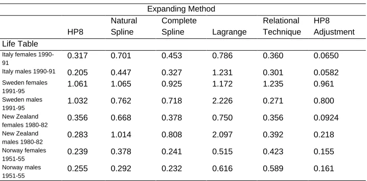
Table 2: Values of the sum of squares of the relative deviations between the resulting and the empirical

q

_x -values.

Expanding Method HP8 Natural Spline Complete Spline Lagrange Relational Technique HP8 Adjustment Life Table

Italy females 1990-91

0.317 0.701 0.453 0.786 0.360 0.0650

Italy males 1990-91 _{0.205 0.447 0.327 1.231 0.301 0.0582} Sweden females

1991-95

1.061 1.065 0.925 1.172 1.235 0.961

Sweden males

1991-95 1.032 0.762 0.718 2.226 0.271 0.800 New Zealand

females 1980-82

0.356 0.668 0.378 0.750 0.356 0.0924

New Zealand males 1980-82

0.283 1.014 0.808 2.097 0.392 0.218

Norway females 1951-55

0.239 0.378 0.241 0.515 0.423 0.155

Norway males 1951-55

Figure 1: Empirical

q

_x– values (points) and estimations by (1) the HP8 formula (solid line), (2) the complete cubic spline interpolation (solid line), (3) the natural cubic spline interpolation (solid line), (4) the Lagrangean interpolation (solid line), (5) the non-parametric relational technique (solid line) and (6) the HP8 adjustment, for Italian males 1990-91.

(1)-HP8

(2)- Complete Spline

age x

100 90 80 70 60 50 40 30 20 10 0

ln(qx*100000)

10

9

8

7

6

5

4

3

2

1

0

Italy 1990-91

age x

100 90 80 70 60 50 40 30 20 10 0

ln(qx*100000)

10 9 8 7 6 5 4 3 2 1

(3)-Natural Spline (4) Lagrangean interpolation

(5) Relational technique (6) HP8 adjustment

age x 80 70 60 50 40 30 20 10 0 ln(qx*100000) 9 8 7 6 5 4 3 2 1 0 Italy 1990-91 age x 100 90 80 70 60 50 40 30 20 10 0 ln(qx*100000) 10 9 8 7 6 5 4 3 2 1

0 Italy 1990-91

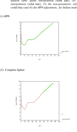
Figure 2: Empirical

q

_x– values (points) and estimations by (1) the HP8 formula (solid line), (2) the complete cubic spline interpolation (solid line), (3) the natural cubic spline interpolation (solid line), (4) the Lagrangean interpolation (solid line), (5) the non-parametric relational technique (solid line) and (6) the HP8 Adjustment, for Norwegian females 1951-55.

(1)- HP8

(2)- Complete Spline

age x

80 70 60 50 40 30 20 10 0

ln(qx*100000)

9

8

7

6

5

4

3

2

1

0 Norway 1951-55

age x

80 70 60 50 40 30 20 10 0

ln(qx*100000)

9

8

7

6

5

4

3

2

1

(3)- Natural Spline (4) Lagrangean interpolation

(5) Relational technique 6)- HP8 Adjustment

age x 80 70 60 50 40 30 20 10 0 ln(qx*100000) 9 8 7 6 5 4 3 2 1

0 Norway 1951-55

age x 60 50 40 30 20 10 0 ln(qx*100000) 8 7 6 5 4 3 2 1

0 Norway 1951-55

age x 60 50 40 30 20 10 0 ln(qx*100000) 8 7 6 5 4 3 2 1

0 Norway 1951-55

age x 80 70 60 50 40 30 20 10 0 ln(qx*1000000 9 8 7 6 5 4 3 2 1

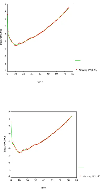
Figure 3: Empirical

q

_x– values (points) and estimations by the reduced HP8 formula (solid line), for Norwegian females 1951-55.

age x

80 70 60 50 40 30 20 10 0

ln(qx*1000000

9

8

7

6

5

4

3

2

1

References

Abramowitz, M, I. A. (1965). Handbook of Mathematical Functions with formulas, Graphs, and Mathematical Tables, National Bureau of Standards, Applied Mathematics Series 55, 4th printing. Washington, D.C.: U.S. Government Printing Office.

Barkalov, N. B. (1988). Interpolation of demographic data using rational spline functions. Demograficheskie Issledovaniya, 44-64. (In Rus.)

Beers, S.H. (1944). Six - term formulae for Routine Actuarial Interpolation, R.A.I.A., 33(2), 245-260.

Benjamin, B. and Pollard, J.H. (1980). The Analysis of Mortality and other Actuarial Statistics, second edition, Heinemann, London.

Bergström, T. and Lamm, D.(1989). Recovering Event Histories by Cubic Spline Interpolation, Mathematical Population Studies, 1(4), 327-355.

Biller, C. and Färhmeir, L. ( 1997). Bayesian Spline - type smoothing in generalized regression models, Computational Statistics, 12, 135-151.

Chambers, J.M. and Hastie, T.J. (1992). Statistical Models in S, Chapman&Hall ed., New York.

Congdon, P. (1993). Statistical Graduation in Local Demographic Analysis and Projection, Journal of the Royal Statistical Society A, 156, 237-270.

DeBoor, C. (1978). A Practical Guide to Splines. Springer-Verlag. New York.

Elandt-Johnson, R., Johnson, N. (1980). Survival Models and Data Analysis, New York, John Wiley.

Forfar, D.O. and Smith, D.M. (1987). The changing shape of the English life tables, Transactions of the Faculty of Actuaries, 40(1), 98-134.

Green, P.J. and Silverman, B.W. (1995). Nonparametric regression and generalized linear models: A roughness penalty approach, Chapman&Hall ed., London.

Greville, T.N.E. ( 1969). Theory and Applications of Spline Functions, New York Academic Press.

Härdle, W. (1992). Applied Non Parametric Methods, CORE Discussion Paper 9203, Universite Catholique de Louvain, Louvain - la - Neuve, Belgium.

Heligman, L. and Pollard, J.H. (1980). The Age pattern of mortality, Journal of the Institute of Actuaries, 107, 49-77.

Hsieh, J.J. (1991). Construction of Expanded Continuous Life Tables - A

Generalization of Abridged and Complete Life Tables, Mathematical

Biosciences, 103, 287-302.

Hsieh, J.J. (1991). A general theory of life table construction and a precise life table method, Biometrical Journal, 33(2), 143-162.

Karlis, D., Kostaki, A. (2000), Bootstrap techniques for mortality models, Technical Report, No 116, Athens University of Economics and Business, Department of Statistics, Greece.

King, G. (1914). On a Short Method of constructing an Abridged life table, 48, J.I.A.294-303.

Kostaki, A. (1987).The Heligman - Pollard formula as a technique for expanding an abridged life table". Department of Statistics, University of Lund, Sweden. Technical report CODEN:LUSADG/SAST-3095/1-44.

Kostaki, A. (1991). The Heligman - Pollard Formula as a Tool for Expanding an Abridged Life Table, Journal of Official Statistics, 7(3), 311-323.

Kostaki, A. (1992a). A nine parameter version of the Heligman-Pollard formula, Mathematical Population Studies, 3(4), 277-288.

Kostaki, A. (1992b). Methodology and Applications of the Heligman-Pollard formula.University of Lund, Department of Statistics. Doctoral dissertation.

Kostaki, A., Lanke, J. (2000). Degrouping Mortality Data for the Elderly. Mathematical Population Studies, 7(4), 331-341.

Kostaki, A. (2000). A Relational Technique for Estimating the age - specific mortality pattern from grouped data, Mathematical Population Studies, 9(1), 83-95.

Lytrokapi, A. (1998). Parametric Models of Mortality: Their use in Demography and Actuarial Science, MSc Dissertation, Athens University of Economics and Business, Department of Statistics, Athens, Greece.

McCutcheon, J.J. and Eilbeck, J.C. (1977). Experiments in the Graduation of the English Life Tables (No. 13) Data, Transactions of the Faculty of Actuaries, 35, 281-296.

McNeil, D.R., Trussel, T.J. and Turner, J.C. (1977). Spline Interpolation of Demographic Data, Demography, 14(2), 245-252.

Namboodiri, K. (1991): Demographic Analysis: A Stochastic Approach. Academic Press, Inc.

Nanjo, Z. (1986). Practical Use of Interpolatory Cubic and Rational Spline Functions for Fertility Data, NUPRI Research Paper Series No. 34, vi, 13pp, Nihon University, Population research Institute, Tokyo, Japan.

Nanjo, Z. (1987). Demographic data and spline interpolation, Journal of Population Studies, No. 10, 43-53 pp. Tokyo, Japan. (In Jpn. with sum. In Eng.)

Pollard, J.H. (1989). On the derivation of a full life table from mortality data recorded in five-year age groups, Mathematical Population Studies, 2(1),1-14.

Renshaw, A.E. (1995). Graduation and Generalized Linear Models: An Overview, Actuarial Research Paper No. 73, City University, Department of Actuarial Science and Statistics, London, UK.

Rogers, A. (1986). Parameterized Multistate Population Dynamics and Projections, Journal of the American Statistical Association, 81, 48-61.

Tyrtyshnikov, E.E. (1997). A Brief Introduction to Numerical Analysis, Birkhauser ed., Boston.

United Nations (1988a). MORTPAK. The United Nations Software Package for

Mortality Measurement (Batch oriented Software for the Mainframe Computer), New York: United Nations, 114-118.

United Nations (1988b). MORTPAK-LITE. The United Nations Software Package for Mortality Measurement (Interactive Software for the IBM-PC andCompatibles), New York: United Nations, 111-114.

Wegman, J.E. and Wright, W.I. (1983). Splines in Statistics, Journal of the American Statistical Association, 78, 351-365.