DEMOGRAPHIC RESEARCH
VOLUME 30, ARTICLE 58, PAGES 1591–1620
PUBLISHED 21 MAY 2014
http://www.demographic-research.org/Volumes/Vol30/58/ DOI: 10.4054/DemRes.2014.30.58
Research Article
Multistate event history analysis with frailty
Govert E. Bijwaard
This publication is part of the Special Collection on “Multistate Event History Analysis,” organized by Guest Editors Frans Willekens and Hein Putter.
c
2014 Govert E. Bijwaard.
2 Frailty in event history models 1594
2.1 Frailty in univariate event history models 1594
2.2 Frailty in multivariate event history models 1595
2.3 Frailty in recurrent events models 1597
3 Frailty in multistate models 1599
3.1 Multistate model concepts 1599
3.2 Frailty in the illness-death model 1601
3.3 General multistate models with frailty 1602
4 Empirical illustration 1606
4.1 Four states model for labour market and migration dynamics 1607
5 Identification issues in multistate frailty models 1614
6 Summary and concluding remarks 1616
Multistate event history analysis with frailty
Govert E. Bijwaard1
Abstract
BACKGROUND
In survival analysis a large literature using frailty models, or models with unobserved heterogeneity, exists. In the growing literature and modelling on multistate models, this issue is only in its infant phase. Ignoring frailty can, however, produce incorrect results.
OBJECTIVE
This paper presents how frailties can be incorporated into multistate models, with an em-phasis on semi-Markov multistate models with a mixed proportional hazard structure.
METHODS
First, the aspects of frailty modeling in univariate (proportional hazard, Cox) and mul-tivariate event history models are addressed. The implications of choosing shared or correlated frailty is highlighted. The relevant differences with recurrent events data are covered next. Multistate models are event history models that can have both multivariate and recurrent events. Incorporating frailty in multistate models, therefore, brings all the previously addressed issues together. Assuming a discrete frailty distribution allows for a very general correlation structure among the transition hazards in a multistate model. Although some estimation procedures are covered the emphasis is on conceptual issues.
RESULTS
The importance of multistate frailty modeling is illustrated with data on labour market and migration dynamics of recent immigrants to the Netherlands.
1Netherlands Interdisciplinary Demographic Institute (NIDI), PO Box 11650, 2502 AR The Hague, The
Netherlands; Phone: (+31) 70 3565 224; Fax: (+31) 70 3647187; E-Mail: [email protected].
1.
Introduction
Demographers are increasingly interested in understanding life histories or the individual life course, with a focus on events, their sequence, ordering and transitions that people make from one state of life to another. A multistate model describes the transitions people experience as life unfolds. When people may change among a set of multiple states and/or may experience repeated changes through time, a multistate event history model, also known as multistate lifetable and increment-decrement life tables, is a proper choice. Typ-ical examples of such processes in demography include migration, (Rogers 1975; 1995), changes in marital status and other life course processes, (Courgeau and Lelièvre 1992 and Willekens 1999). Many other demographic applications of the multistate models exist. Multistate models are also common in medicine and economics. In medicine, the states can designate conditions such as healthy, diseased and death. For an overview of the use of multistate models in biostatistics, see a.o. Commenges (1999), Hougaard (2000), and Putter, Fiocco, and Geskus (2007). In economics the main application of multistate models has been labour force dynamics; see Flinn and Heckman (1983), Van den Berg (2001) and, Fougère and Kamionka (2008). Poverty dynamics and recidivism are other important applications of multistate models. The methodology of multistate models is dis-cussed in several books; the most important are Andersen et al. (1993), Hougaard (2000), and Aalen, Borgan, and Gjessing (2008).
In our empirical application we focus on the return decision of labour migrants and its relation to labour market dynamics. Many migrants only stay temporarily in the host country. On the one hand, return migration is seen as planned and part of optimal decision making to maximize total utility over the whole life cycle, where return migration is mo-tivated by locational preference for the home country. On the other hand, return migration is seen as unplanned and the result of failure either due to imperfect information about the host country in terms of labor market prospects or the cost of living, or the inability to fulfil the migration plans in terms of target savings. In both cases, return behaviour is intrinsically related to the timing of labour market changes of the individual migrant. Migrants who become unemployed are more prone to leave, but when they find a new job again they are more prone to stay, see Bijwaard, Schluter, and Wahba (2014). Migrants who are employed in high paying jobs have a lower probability of becoming unemployed and can accumulate more savings while working. When these migrants have reached tar-get savings they are more prone to leave, see Bijwaard and Wahba (2014). Labour market dynamics may also be affected by the labour market history. These factors suggest that return migration behaviour of labour migrants should be modeled by a multistate model.
inten-sities are homogeneous, conditional on these observed factors. Unfortunately, it is hardly ever possible to include all relevant factors, either because the researcher does not know all the relevant factors, or because it is not possible to measure all the relevant factors. Ignoring such unobserved heterogeneity or frailty may have a large impact on inference in multistate models. The duration dependence, the effect of the length of the duration in a particular state on the exit rate out of this state, will be biased towards a more declining ef-fect of the duration when frailty is ignored. The efef-fect of covariates on the transition rates will be biased towards zero when frailty is ignored. For univariate event history data, also called survival data or duration data, a large literature on models with frailty exits, e.g. Van den Berg (2001), Duchateau and Janssen (2008) and Wienke (2011). In the multistate literature, the issue of including frailty is only in its infant phase. The few articles that deal with frailty in multistate models are Pickles and Crouchley (1995), Govindarajulu et al. (2011) and Putter and van Houwelingen (2011).
The purpose of this article is to provide an overview of frailty modeling for multistate event history models. We assume that the frailty for all members, just as the effect of observed characteristics, enters the intensity multiplicatively. Thus, we only consider the Cox model in continuous time with frailty, in econometrics called the Mixed Proportional Hazard model, and its multivariate extensions.
The outline of the paper is as follows. In Section 2. we start with a discussion on the issues involved in frailty in univariate survival models. Multistate models extend the univariate survival models in two dimensions: (1) Several people that may experience an event may be grouped in clusters. Note that this is conceptually equal to the situation in which for one individual several processes are followed simultaneously. In both cases we have parallel events. (2) People may experience multiple periods of the same type or recurrent events. In both dimensions, frailties can be independent, shared, or corre-lated. We also discuss these issues separately for parallel and for recurrent event data. In Section 3. frailties in a multistate setting are addressed, combining the knowledge of the preceding section on incorporating frailties in models for parallel data and in models for recurrent data. In Section 4. we illustrate the importance of incorporating frailty in a semi-Markov multistate model with data on labour market and migration dynamics of re-cent immigrants to the Netherlands. In Section 5. we briefly discuss identification issues in multistate frailty models. Section 6. summarizes the findings.
2.
Frailty in event history models
2.1 Frailty in univariate event history models
The simplest multistate model is a univariate survival model, which considers the transi-tion from ‘alive’ to ‘dead’, or return migratransi-tion, in our running example. The observatransi-tion for a given individual will in this case consist of a random variableT, representing the time from a given origin (time 0) to the occurrence of the event ‘death’. The distribution ofT may be characterized by the survival function S(t) = Pr(T > t). We can also characterize the distribution ofT by its hazard rateλ(t), which is the transition intensity from state ‘alive’ to state ‘dead’, i.e. the instantaneous probability per time unit of going from ‘alive’ to ‘dead’. The hazard rate provides a full characterization of the distribution ofT, just like the distribution function, the survival function, and the density function.
A typical feature of event history analysis is the inability to observe complete event histories. A common problem is that by the end of the observation period, some individu-als still have not yet experienced the event of interest. This kind of incomplete observation is known as right-censoring. The hazard function is usually the focal point of analysis. A major advantage of using the hazard function as the basic building block is that it is invariant to independent censoring. The most common model for the hazard rate is the Cox or proportional hazard (PH) model, with hazard rate
λ(t|X) =λ0(t) exp(β0X), (1)
whereλ0(t)is called the baseline hazard or duration dependence and it is a function oft
alone.
In a Mixed Proportional Hazard (MPH) model it is assumed that all unmeasured fac-tors and measurement errors can be captured in a multiplicative random term, the frailty
V. The hazard rate becomes
λ(t|X, V) =V λ0(t) exp(β0X). (2)
This model was independently developed by Vaupel, Manton, and Stallard (1979) and by Lancaster (1979). The frailtyV >0is time-independent and independent of the observed characteristicsX.
hazard rate exhibits negative duration dependence, ignoring frailty will make this negative duration dependence stronger. Another consequence of ignoring frailty is that the effect of a covariate is biased towards zero.
The most commonly used frailty distributions are the Gamma frailty distribution, the log-normal frailty distribution, and the discrete frailty distribution. For more details on these and other frailty distributions, like the Power Variance Function family of frailty distributions that includes the important Inverse Gaussian and Stable frailty distributions I refer to Hougaard (2000) and Wienke (2011).
The Gamma distribution is the most widely applied frailty distribution. From an an-alytical and computational view it is a very convenient distribution. The closed form expressions for the unconditional survival and hazard are easy to derive. The link with random effects or mixed models makes the log-normal model very attractive. A disad-vantage is the lack of closed form expressions. But with increasing computer power the numerical solution of the integrals involved is not an issue anymore.
The discrete frailty model, in which it is assumed that the population consists of two, or more, latent sub populations, which are homogeneous within, is a finite mixture model. For example we may have (1) a high risk subpopulation that leaves fast, and (2) a low risk subpopulation that leaves slowly, but the class identification for each individual is unknown. In econometrics such frailty models are commonly applied in survival analysis.
2.2 Frailty in multivariate event history models
There are two typical ways multivariate event history data can arise. The first situation of multivariate event history data isparallel event history data, in which for one individual several processes are followed simultaneously. A typical parallel events data example is the competing risks model of different causes of death or of exits from employment to either unemployment or non-participation. Data in which several individuals that may experience an event are grouped in a cluster are conceptually the same with parallel data. Examples of such data include twin and family studies. The second situation of multi-variate event history data isrecurrent/repeated eventswhich arises when several events of the same type are registered for each individual, for instance child birth to a woman, or periods of unemployment. In univariate event history models frailty captures the possible heterogeneity due to unobserved covariates. In a multivariate setting frailty can also be used to model associations between events, but events from different clusters are consid-ered to be independent.
A key point for an MPH model is conditional independence, that is conditional on the frailtyv the survival times are independent. In the multivariate setting we continue to assume the MPH structure and the conditional independence. In principle the frailty
might be independent for each event. Then the analysis does not differ from the analysis in a univariate setting. Here we consider the more interesting cases of (1) shared frailty and (2) correlated frailty.
The shared frailty approach assumes that within a cluster, the value of the frailty term is constant over time, and common to all individuals in the cluster. Examples include: the frailty in the transition from employment to unemployment is equal to the frailty in the transition from employment to non-participation, and the frailty in the death rate for all members of one family are the same. This common term, creates dependence between event times within a cluster. This dependence is always positive. The shared frailty model, first introduced by Clayton (1978), dominates the literature on multivariate survival models, see Hougaard (2000), Therneau and Grambsch (2000) and Duchateau and Janssen (2008), among others.
Despite the similarity between individual frailty and shared frailty conceptually they are different. In the univariate case, the frailty varianceσ2is a measure of unobserved
heterogeneity, while in a shared frailty multivariate case, the frailty variance is a measure of correlation between event times within a cluster.
The shared frailty model, with a shared Gamma frailty distribution as most popular choice, has some important limitations; see Xue and Brookmeyer (1996) for an extensive discussion. First, the assumption that the frailty is the same for all members in the clus-ter is often inappropriate. Second, shared frailty models only induce positive association within clusters. However, in some situations, the event times for individuals within the same cluster are negatively associated. For example, the reduction in the risk of dying from one disease may increase the risk of dying from another disease. Third, the depen-dence between survival times within a cluster is based on marginal distributions of event times. This leads to a symmetric relationship between all possible pairs within a cluster. It also limits the interpretation of the variance of the shared frailty model as a measure of association between event times within a cluster, and not as a measure of unobserved heterogeneity. Correlated frailty models allow more flexibility.
In a correlated frailty model the frailties of individuals within a cluster are correlated but not necessarily shared. It enables the inclusion of additional correlation parameters and associations are no longer forced to be the same for all pairs of individuals within a cluster. We consider three different ways of generating correlated frailties: (i) additive frailty in which the frailty is the sum of a cluster-specific and an individual-specific com-ponent; (ii) nested frailty, in which the frailty is the multiplication of a cluster-specific and an individual-specific component; and (iii) joint modeling of the member specific frailties within a cluster. In all three cases the conditional survival still has an MPH structure.
history model with additive gamma frailty. Each frailty is constructed by adding two components, one common to both and one individual specific. A consequence of the model structure is that when the values of the variances of the two individual terms differ a lot the correlation cannot be very large. Another disadvantage of the additive correlated gamma frailty is that estimation of the model becomes very complex with increasing cluster size.
The nested frailty model assumes that the clustering of the event times occurs at multiple levels. In family studies, where we have a hierarchical clustering by family and individual, this models seems appropriate. Sastry (1997a) suggested a nested frailty model with two hierarchical levels in which the frailty of memberjin a particular cluster is Vj = W0 ·Wj withW0 andWj are mutually independent unit-mean gamma dis-tributed random variables with varianceη0 andη1. Thus, within each cluster the frailty
is composed of a cluster-specific component common to all cluster members times an individual-specific component that are mutually independent. The unconditional survival for this nested gamma frailty has a complicated form, but estimation is possible using an EM-algorithm (Sastry 1997a; 1997b), a Bayesian procedure (Manda 2001) or penalized likelihood methods (Rondeau, Commenges, and Joly 2003).
A very flexible way to allow for correlated frailties is by modeling the joint frailty
distribution directly. The correlated log-normal frailty model, first applied by Xue and Brookmeyer (1996), is especially useful in modeling dependence structures. The distri-bution can be obtained by assuming a multivariate normal distridistri-bution on the logarithm of the frailty vector. However, the log-normal distribution does not have analytical solutions for the unconditional joint survival and hazards, and the number of integrals to evaluate for calculating them increases with the dimension of the multivariate normal distribution. Assuming a joint discrete frailty distribution is another way to allow for correlation between the frailties. However, in an unstructured discrete frailty model the number of (additional) parameters increases fast. This dimensional burden can be reduced by assuming a factor loading specification, e.g. 2-factor loading model in which Vj = exp(αj1W1+αj2W2)withW1 andW2 are binary mutually independent variables on
(−1,1)withpk =P r(Wk= 1).
2.3 Frailty in recurrent events models
Another extension of the univariate survival model is that an individual can experience the same event several times, e.g. become repeatedly unemployed. Reviews of models for such recurrent event data appeared in Cook and Lawless (2007). Recurrent data can be represented in different ways depending on the timescale that is used; (i) gap time, or clock reset time; (ii) total time, or clock forward time, see e.g. Kelly and Lim (2000).
Related to the choice of the time scale are therisk-intervaland the risk set. The risk interval corresponds to the time interval where an individual is at risk of experiencing an event. The risk set is the collection of individuals which are at risk at a certain point in time. In the gap-time representation, time at risk starts at 0 after an event and ends at the time of the next event. Hence, time is reset to zero after each event. In the total-time formulation, the length of the time at risk is the same as in the gap-time representation. The difference is that the starting time of the at-risk period is not reset to zero after an event but it is put equal to the actual time since the beginning of the observation period.
Based on the choice of the risk set, the three most common approaches to recurrent events are the independent increment model of Andersen and Gill (1982), the marginal model of Wei, Lin, and Weissfeld (1989), and the conditional model of Prentice, Williams, and Peterson (1981); see Kelly and Lim (2000) for a comparison. For the marginal and conditional models, each occurrence of the event is modeled as a separate event, while the independent increment model assumes that the occurrence of an event of one individual is independent of the number and timing of previous events. The independent increments model is usually defined in total time, but it can also be formulated in gap time. This model assumes that the gap times are generated from a renewal process. In essence, the marginal model treats the consecutive event times as if they come from an unordered com-peting risk setting, with the number of occurrences at the number of comcom-peting events. The marginal model can only be formulated in total time. The conditional model assumes that an individual cannot be at risk for the second occurrence of an event until the event has occurred for the first time.
Nielsen et al. (1992) discuss how to include frailty in the independent increments model. In Chapter 9 of his seminal book, Hougaard (2000) also discusses shared frailty models for recurrent events in which the frailty is shared over time. Frailty models spe-cially designed for recurrence data are considered in detail in Oakes (1992), Duchateau et al. (2003) and Bijwaard, Franses, and Paap (2006). For recurrent events the frailty variation is not a group variation, but a variation between individuals, and the variation described by the hazard function is not an individual variation but a variation within indi-viduals. The interpretation of the frailty variance also depends on the time scale and risk sets used.
3.
Frailty in multistate models
A multistate model is defined as a stochastic process, which at any point in time occupies one of a set of discrete states. The class of multistate models includes both recurrent and multivariate event history data. For example, in labour force dynamics, multiple (un)employment periods are recurrent events and the states are multivariate because from a state of employment an individual can either become unemployed or leave the labour market. In that respect special cases of a multistate model are the multivariate parallel and recurrent models in the previous section. Thus, including frailty in multistate models follows the lines of the previous sections. Before introducing multistate models with frailty we explain the main concepts of multistate models.
3.1 Multistate model concepts
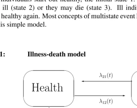
The most commonly applied multistate model in biostatistics is the illness-death model (Putter, Fiocco, and Geskus 2007). This model is depicted in Figure 1. In this class of models individuals start out healthy, the initial state 1. From a healthy state they may become ill (state 2) or they may die (state 3). Ill individuals may die or recover and become healthy again. Most concepts of multistate event history analysis can be explained using this simple model.
Figure 1: Illness-death model
Health
' & $ %-λ12(t)
@ @ @ @ @ @ @ @
@@R
λ13(t)
Illness
'&
$
%
λ21(t)
λ23(t)
Death
'&
$
%
Figure 1: Illness-death model
3
Frailty in multistate models
A multistate model is defined as a stochastic process, which at any point in time occupies one of
a set of discrete states. The class of multistate models includes both recurrent and multivariate
event history data. For example, in labour force dynamics multiple (un)employment spells
are recurrent events and the states are multivariate because from employment an individual
can either become unemployed or leave the labour market. In that respect special cases of a
multistate model are the multivariate parallel and recurrent models in the previous section.
Thus, including frailty in multistate models follows the lines of the previous sections. Before
introducing multistate models with frailty we explain the main concepts of multistate models.
3.1 Multistate model concepts
The most commonly applied multistate model in biostatistics is the illness-death model (Putter,
Fiocco, and Geskus 2007). This model is depicted in Figure 1. In this class of models individuals
start out healthy, the initial state 1. From healthy they may become ill (state 2) or they may
die (state 3). Ill individuals may die or recover and become healthy again. Most concepts of
multistate event history analysis can be explained using this simple model.
Multistate modeling is closely related to Markov chain theory and many of its terminology
originate from the theory of Markov chains and processes. Most multistate models have three
Multistate modeling is closely related to Markov chain theory and many of its terms originate from the theory of Markov chains and processes. Most multistate models have three states: the initial state(s), the states in which an individual can enter the study; absorbing states, states that represent an endpoint from which the individual cannot leave or one is not interested in what happens after this state has been reached; intermediate or transient states are all other states. In an illness-death model death is an absorbing state and illness is an intermediate state. The multistate event history model is defined in hazard/transitions rates. We denote the hazard of making a transition from stateito state
j(i6=j) attbyλij(t).
Just as for recurrent events, the choice of the time scale in a multistate model has important implications for the analysis. In a total time representation the event times,t, correspond to the time since the individual entered the initial state. The time keeps moving forward, both when intermediate events occur or when the individual returns to the initial state. In a gap time representation, the event times correspond to the time since the entry in statei. The time is reset to zero each time an individual makes a transition. Gap time is also called sojourn time, clock reset time and backward recurrence time. The time scale chosen has implications for the risk set that defines who are at risk for a particular event, for a transition within a multistate framework.
to mixed proportional hazard type transition rates and assume that, conditionally on the value of the frailty, the semi-Markov property holds.
3.2 Frailty in the illness-death model
We illustrate the choices involved in including frailty in multistate models by using the illness-death model. In the illness-death model we have four transitions rates
λ12(t|X12, v12) = v12λ012(t) exp(β12X12) from healthy to ill (3)
λ13(t|X13, v13) = v13λ013(t) exp(β13X13) from healthy to death (4)
λ21(t|X21, v21) = v21λ021(t) exp(β21X21) from ill to healthy (5)
λ23(t|X23, v23) = v23λ023(t) exp(β23X23) from ill to death, (6)
whereX12, X13, X21andX23are the observed individual characteristics. The included
covariates might be different for each transition. The baseline hazardsλ012(·), . . . , λ023(·)
depend on the sojourn time in the state, and might be equal for the same origin state. Here we focus on the choice of the frailty distribution. When all the frailties are mutually independent the model reduces to two independent competing risks models. From the healthy state, the competing states the individual can move to are illness and death. From the illness state the individual can either move to healthy or to death. In both cases the competing risks are uncorrelated and the frailty variance is a measure of unobserved het-erogeneity within the origin-destination combination.
An illness-death model with shared frailty model by origin state implies equal frailties from the healthy statev1=v12=v13and equal frailties from the illness statev2=v21=
v23. The frailty variance is in this case a measure of correlation between events times from
either healthy to illness or to death or from illness to healthy or to death.
Concerning correlated frailty models, we have the choice between three different ways of generating correlation between the linked transitions: an additive frailty model, a nested frailty model or a joint frailty model. With correlation based on origin states, we have two sets of mutually independent correlated frailties, the frailties of the healthy state, v12 andv13, and the frailties of the illness state, v21 andv23. With correlation
based on destination states, we have three sets of mutually independent correlated frail-ties: the frailty to the healthy state,v21, the frailty to the illness state,v21and the frailties
to the death state,v13andv23. When all four frailties are correlated, we can use
four-dimensional frailty models. Note that the additive gamma frailty models become very complex for four dimensional frailties. For the discrete correlated frailty models, a
factor loading model specification would leave the parameter space manageable without putting too much restriction on the correlations. An advantage of the discrete model is that it also allows for negative correlations among the unobserved factors. In the proto-typical application of the illness-death model in biostatistics, describing the transitions of patients, this possibility might sound redundant, as factors increasing the rate into illness usually also increase the death rate. However, when the illness-death model is applied to socio-economic transitions, restricting to positive correlation can be very restrictive. For example, labour migrants who are more likely to become unemployed (“ill”) are often less likely to find a new job again (“healthy”).
So far we have ignored possible recurrent behaviour in the model. In the illness-death model, only the health and illness state might be recurrent. But the transition rates to death from these two states may also change with reoccurence. Of course, a simple way to allow for such dependence is to include as an additional covariate the number of times an individual has been in the state. Recurrence may also affect frailties. When the frailties are shared over the occurrences, the possible models are basically the same as mentioned above, with the only difference is that the baseline duration and the regression function are stratified by occurrence. When the frailties are independent over the recurrence, i.e. each recurrence has a separate frailty, the model is just a repeated version of the model above. When allowing a more flexible correlation the possible frailty structures becomes rather large. In principle an extension of the autocorrelated frailty model of Yau and McGilchrist (1998) to the illness-death model is possible. We assume that the frailty is shared or independent over the occurrences.
3.3 General multistate models with frailty
For general multistate models beyond the simple illness-death model, many alternative correlation structures for the frailties are possible. In principle, a multistate model has three dimensions; the origin states, the destination states and the recurrent events of a particular state. The hazard from stateito statej(i6=j) for thekthtime is
λijk(t|X, Vijk) =Vijkλijr0(t) exp(βijk0 Xijk).
Of course, it is allowed to put restrictions on the duration dependence, on the observed characteristics or on the effect of the observed characteristics on the hazard. For example, the duration dependence might be shared for all exits of one origin state, λijr0(t) =
λir0(t), the observed characteristics might be shared over all recurrent events,Xijk =
Table 1: Possible correlation structures of frailty in a multistate model
Origin-destination Recurrent structure
structure independent shared
Fully ρ vijk, virk
=0 ρ vijk, virk
=0 independent ρ vijk, vmjk
=0 ρ vijk, vmjk
=0
ρ vijk, vmrk
=0 ρ vijk, vmrk
=0
ρ vijk, vijg
=0 ρ vijk, vijg
=1
Shared ρ vijk, virk
=1 ρ vijk, virk
=1 over origin ρ vijk, vmjk
=0 ρ vijk, vmjk
=0
ρ vijk, vmrk=0 ρ vijk, vmrk=0
ρ vijk, vijg =0 ρ vijk, vijg =1 Shared ρ vijk, virk =0 ρ vijk, virk =0 over destination ρ vijk, vmjk=1 ρ vijk, vmjk=1
ρ vijk, vmrk
=0 ρ vijk, vmrk
=0
ρ vijk, vijg
=0 ρ vijk, vijg
=1
Fully ρ vijk, virk
=1 ρ vijk, virk
=1 shared ρ vijk, vmjk
=1 ρ vijk, vmjk
=1
ρ vijk, vmrk
=1 ρ vijk, vmrk
=1
ρ vijk, vijg
=0 ρ vijk, vijg
=1
Correlated ρ vijk, virk
=ρij,ir ρ vijk, virk
=ρij,ir over origin ρ vijk, vmjk
=0 ρ vijk, vmjk
=0
ρ vijk, vmrk
=0 ρ vijk, vmrk
=0
ρ vijk, vijg
=0 ρ vijk, vijg
=1
Correlated ρ vijk, virk =0 ρ vijk, virk =0 over destination ρ vijk, vmjk=ρij,mj ρ vijk, vmjk=ρij,mj
ρ vijk, vmrk=0 ρ vijk, vmrk=0
ρ vijk, vijg =0 ρ vijk, vijg =1 Fully ρ vijk, virk
=ρij,ir ρ vijk, virk
=ρij,ir correlated ρ vijk, vmjk
=ρij,mj ρ vijk, vmjk
=ρij,mj
ρ vijk, vmrk
=ρij,mr ρ vijk, vmrk
=ρij,mr
ρ vijk, vijg
=0 ρ vijk, vijg
=1
With independent frailty, we have for each origin-destination-recurrence pair, vijk, an independent frailty, and all frailties are uncorrelated. This is, for example, the case when all transitions in a labour-dynamics return migration multistate model are only
related through observed characteristics. Table 1 provides the possible tractable correla-tion structures when changing the dependence in all three dimensions. The first column gives the correlation structure when the frailties are independent over the recurrences and the second column when the frailties are shared over the recurrences. When the frailties are shared over recurrences, the correlation between two frailties of different occurrence,
ρ vijk, vijg
, is one. When the frailty is shared over the origin state and independent over recurrences, i.e. all destinations from one origin share the same frailty but not over recurrences, then the frailty distribution only depends on the origin stateiand the corre-lation between two frailties from the same origin,ρ vijk, virk
, is one. For example, this amounts to dependence of the transition hazards to unemployment, non-participation and abroad from employment for a particular employment period, but independence of these hazards for different employment periods. When the frailty is shared over the destination state and independent over recurrences, i.e. hazards to one particular destinations share the same frailty but not over recurrences, then the frailty distribution only depends on the destination statej and the correlation between two frailties to the same destination,
ρ vijk, vmjk
, is one. When the frailty is shared over origin, destination and recurrence states we have only one frailty value for each individual and therefore the correlation is one.
When the frailties are correlated over origin states the frailties from the same origin
ito different destinationsj andrare correlated and depend on the destination state, i.e.
ρ vijk, virk
=ρij,ir. When the frailties are correlated over destination states the frailties to the same destinationjfrom different originsiandmare correlated and depend on the origin state, i.e.ρ vijk, vmjk
=ρij,mj. When the frailties are correlated over both origin and destination states the correlation is defined in all possible origin-destination combina-tions, e.g.ρ vijk, vmrg
=ρij,mr. The first situation, correlated over origin, implies that the hazard from employment to unemployment, from employment to non-participation and from employment to living abroad are correlated through the frailty term, while the hazards from unemployment to either employment, non-participation or moving abroad are uncorrelated with the out-off-employment hazards. In the second situation, correlated over destination, the hazards to employment, from unemployment, from non-participation and from abroad are all correlated through frailty. In the third situation, full correlation, the hazards from employment, from unemployment, from non-participation and from liv-ing abroad to all other states are all correlated through the frailty.
model with frailty
vijk = M
Y
m=1
expα(ijkm)·Wijk(m), (7)
whereWijk(1), . . . , Wijk(M)are M binary variables mutually independent on(−1,1)with
pijk = P r(Wijk = 1). For example, in a 2-factor loading model each frailty can at-tain four different values,{eα1+α2, e−α1+α2, eα1−α2, e−α1−α2}. In general, anM-factor
loading model allows for2M possible values for each frailty. In Table 2 we display the restrictions on the factor loading and number of factors implied by the alternative corre-lation structures of Table 1.
Consider, for example, a discrete frailty 2-factor loading model. Table 2 shows that when a separate model is defined for each origin, i.e. separate Wi’s for each origin, the frailty is shared over recurrence and correlated or shared over origin. The frailty is shared over the origin states when the factor loadings are the same for each destination,
α(ijm)=α(im). Similarly, when we have a 2 factor model with factor loadings depending on the origin and destination state, the frailties are fully correlated over the origin and destination states. Note that for these factor loading models, the shared frailty models are nested in the correlated frailty models. A fully shared model is nested in a fully correlated model, and a shared over the origin model is nested in a correlated over origin states model. This implies that testing the equality of the relevantα’s is a test on correlated versus shared frailties.
Table 2: Restrictions implied by correlation structure on factor loadings and number of factors for a discrete frailty factor loading model
Origin-destination Recurrent structure
structure independent shared
Fully α(ijkm)=αijk(m) α(ijkm)=α(ijm)
independent Wijk(m)=Wijk(m) Wijk(m)=Wij(m)
Shared α(ijkm)=αik(m) α(ijkm)=α(im)
over origin Wijk(m)=Wik(m) Wijk(m)=Wi(m)
Shared α(ijkm)=αjk(m) α(ijkm)=α(jm)
over destination Wijk(m)=Wjk(m) Wijk(m)=Wj(m)
Fully α(ijkm)=αk(m) α(ijkm)=α(m)
shared Wijk(m)=Wk(m) Wijk(m)=W(m)
Correlated α(ijkm)=αijk(m) α(ijkm)=α(ijm)
over origin Wijk(m)=Wik(m) Wijk(m)=Wi(m)
Correlated α(ijkm)=αijk(m) α(ijkm)=α(ijm)
over destination Wijk(m)=Wjk(m) Wijk(m)=Wj(m)
Fully α(ijkm)=αijk(m) α(ijkm)=α(ijm)
correlated Wijk(m)=Wk(m) Wijk(m)=W(m)
Notes: Origin statei6=m, destination statej 6=rand recurrent eventk6=g. Factor discrete model: vijk =
QM m=1exp α
(m)
ijk ·W
(m)
ijk
withW ={−1,1}andPr(Wijk(m)= 1) =p(ijkm).
4.
Empirical illustration
con-junction. We address these issues by using a unique administrative panel for the entire population of recent migrants and estimate a multistate model on the labour market and migration dynamics of these migrants.
To this end we use administrative data from the Netherlands, where we observe all immigrants who have entered the country between 1999 and 2007. Our data comprise the entirepopulationof immigrants who entered during our observation window of 1999– 2007, and after merging in other administrative registers, we obtain a panel. In addition to the date of entry and exit, the administration also records the migration motive of the individual. Either the motive is coded according to the visa status of the immigrant, or the immigrant reports the motive upon registration in the population register. See Bijwaard (2010) for an extensive descriptive analysis of the various migration motives. Here we focus exclusively on 94,270 labour migrants, which comprise about 23% of all non-Dutch immigrants in the age group 18–64 years.
This immigration register is linked by Statistics Netherlands to the Municipal Regis-ter of Population (Gemeentelijke Basisadministratie, GBA) and to their Social Statistical Database (SSD). The GBA contains basic demographic characteristics of the migrants, such as age, gender, marital status and country of origin. From the SSD we have infor-mation, on a monthly basis, on the labour market position, income, employment sector, housing and household situation.
4.1 Four states model for labour market and migration dynamics
We are interested, per se, in the labour market and the migration dynamics, the timing of the transitions and the time between transitions. Since we observe immigrants from the time they enter until the end of our observation window, and since we focus on those employed immigrants at entry, an immigrant potentially faces different risks of exiting his/her first state of employment and multiple durations. We define the following four states: (e) Employed in the Netherlands; (u) Unemployed and receiving benefits in the Netherlands; (n) Out of the labour market (and not receiving benefits = non-participating) in the Netherlands (NP); (a) Living abroad. Table 3 reports the observed transitions among these three labour market states and the living abroad state. Note that by the end of the observation window, 1-1-2008, all migrants are categorized in one of the four states.
Table 3: Spell dynamics of the labour migrants (# 94,270)
Percentage ending in
# of spell employed UI NP Abroad
Employed 124058 43% 5% 42% 10%
Unemployed (UI) 11898 49% 14% 33% 4%
Non-participation (NP) 56559 38% 9% 14% 39%
Abroad 45578 6% 0.2% 2% 92%
Source: Statistics Netherlands, based on own calculations.
Many employment spells are still continuing by the end of the observation period. For the majority of employment spells that end in a transition the migrant leaves the labour market, becomes non-participating. Many non-participation spells end abroad, while many unemployed return to employment. A third of the unemployed receiving benefits leave the labour market. Very few migrants leave the country directly from a state of unemployment. When a migrant leaves the country, they usually remain abroad; they are still abroad at the end of the observation period.
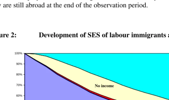
Figure 2: Development of SES of labour immigrants arriving in 1999
Employed Receiving
benefits No income
Abroad
0% 10% 20% 30% 40% 50% 60% 70% 80% 90% 100%
0 4 8 12 16 20 24 28 32 36 40 44 48 52 56 60 64 68 72
By definition all labour migrants start in the employed state at entry. Soon after arrival some migrants move to the other states. Some may return and some may move on to another state. But the migrant is always in one of the four states. In Figure 2 we depict the raw development over time of the distribution over the four states for the 1999-entry cohort, the labour migrants who arrived in 1999. The proportion abroad continuously increases. Six years after arrival more than 50% of the migrants have left the country. The remaining migrants are either employed or non-participating. Only a few migrants get unemployment benefits, possibly because they have not yet gained any benefit rights in the Netherlands.
We view the migrant behavior as a semi-Markov process, with individuals moving between the four states. These states are mutually exclusive and exhaust all possible destinations.2 A migrant may leave a statei={e, u, n, a}for any of the other destination states. The 4-state multistate model is depicted in Figure 3.
Figure 3: Multistate model for labour-migration dynamics
Employed ' & $ % -λeu(t)
? λen(t)
HH HH
HH HH
HHHHj λea(t)
Unemployed '
&
$
%
λue(t)
? λua(t)
λun(t)
Non-participating ' & $ % -λna(t)
6
λne(t)
*
λnu(t)
Abroad '
&
$
%
λan(t)
6
λau(t)
H H H H H H H H H H H H Y
λae(t)
2The mortality rate for the age range 18–64 is small enough to ignore deaths.
We use a competing risks hazard model for each origin-destination pair. We assume that recurrence of the states does not directly affect the frailty or the duration dependence, they are shared over recurrence. Recurrence influence on the hazard is captured by in-cluding the labour-migration history in the covariates. Define the random variablesTij that describe the time since entry inifor a transition fromitoj. We assume a (mixed) proportional hazard model for which the intensity for the transition fromjtokis:
λij(t|Xij(t), vij) =vijλ0ij(t) exp βij0 Xij(t)
(8)
whereXij(t) ={Xij(s)|0 ≤s ≤t}is the sample path of the observed characteristics up to timet, which is, without loss of generality, assumed to be left continuous. For the baseline durationλ0ij(t)we assume that it is piecewise constant on eleven intervals; every six months and beyond five years. Let the intervals Im(t) = I(tm−1 ≤ t <
tm) for m = 1, . . . , M + 1with t0 = 0 andtM+1 = ∞ be the intervals on which
we define the piecewise constant intensity. Then, the baseline intensity is λ0ij(t) =
eβ0ij ·PM+1
m=1 e
αmijI
m(t), withα1ij = 0. Thusβ0ij determines the intensity in the first interval. Theα’s determine the difference in intensity at each interval compared to this first interval. The baseline intensity for a duration oft ∈ [tm−1, tm)is higher than the baseline intensity to leave for a duration oft < t1ifαmij >0and lower ifαmij<0.
We use three different frailty models: (1) a PH model, a model without frailty (PH); (2) uncorrelated MPH model with a two-point discrete frailty (MPH); and (3) a two-factor loading correlated frailty over the origin state (correlated MPH). The covariates included in the model refer to demographic (gender, age-dummies, martial status and age of chil-dren), country of origdummies, individual labour market characteristics (monthly in-come, employment sector-dummies), labour market history and migration history. We control for business cycle conditions by including the national unemployment rate, both at the moment of first entry to the country and the time-varying monthly rate. The un-employment rate at entry captures the ‘scarring effect’ of migrants, while the running unemployment rate captures the impact of the business cycle on the transition intensities. With the abundant information on the migrants, the model contains many parameters. We used maximum likelihood estimation in STATA to estimate all the coefficients.3 Here we
only discuss the parameter estimates of the transition from employed to abroad,λea(t) and, focus on the differences induced by the alternative frailty assumptions.4
3The code is available upon request. The standard errors are calculated using the outer-product of the gradient
vector in the estimated parameter vector. Other alternative estimation procedures for event history models with frailty are: the Expectation-Maximization (EM) algorithm, penalized partial likelihood, and Bayesian Markov Chain Monte Carlo methods.
4All estimation results are available from the author. Related multistate models on similar data are estimated
Table 4: Parameter estimates transition from employed to abroad,λea(t)
space
space Independentspace Correlated
space PHspace MPHspace MPH
female space−0.314∗∗space−0.377∗∗space−0.382∗∗ self-employed space−0.781∗∗space−0.976∗∗space−1.118∗∗ income<1000 space 0.692∗∗space 0.917∗∗space 0.971∗∗ income 1000–2000 space 0.155∗∗space 0.206∗∗space 0.237∗∗ income 3000–4000 space 0.178∗∗space 0.182∗∗space 0.174∗∗ income 4000–5000 space 0.152∗∗space 0.169∗∗space 0.163∗∗ income 5000–6000 space 0.306∗∗space 0.321∗∗space 0.334∗∗ income>6000 space 0.319∗∗space 0.349∗∗space 0.376∗∗ married space−0.147∗∗space−0.175∗∗space−0.220∗∗ divorced space−0.297∗∗space−0.383∗∗space−0.427∗∗ repeated entry space 0.382∗∗space−0.388∗∗space−0.346∗∗ repeated unemployment space−0.376∗∗space−0.303∗ space−0.419∗∗ Unemployment rate at entryspace 0.101∗∗space 0.108∗∗space 0.107∗∗ Unemployment rate space 0.060∗∗space 0.039∗∗space 0.040∗∗
α2(6–12 months) space 0.641∗∗space 0.792∗∗space 0.848∗∗
α3(12–18 months) space 0.694∗∗space 0.945∗∗space 1.036∗∗
α4(18–24 months) space 0.834∗∗space 1.151∗∗space 1.269∗∗
α5(24–30 months) space 0.648∗∗space 1.032∗∗space 1.175∗∗
α6(30–36 months) space 0.750∗∗space 1.198∗∗space 1.363∗∗
α7(36–42 months) space 0.417∗∗space 0.924∗∗space 1.112∗∗
α8(42–48 months) space 0.480∗ space 1.038∗∗space 1.248∗∗
α9(48–54 months) space 0.352∗∗space 0.966∗∗space 1.200∗∗
α10(54–60 months) space 0.263∗∗space 0.921∗∗space 1.180∗
α11(>60 months) space−0.095∗ space 0.669∗∗space 0.987∗
constant (β0) space−6.118∗∗space−5.937∗∗space−5.850∗∗
Source: Statistics Netherlands, based on own calculations.
The estimated duration dependence and covariate effects of λea(t) are reported in Table 4. As expected, ignoring frailty biases the hazard of leaving the country towards
effects of the MPH in a multistate model with uncorrelated frailties. Bijwaard and Wahba (2014) estimate and discuss an extension of the multistate model of this paper in which the wage earned while employed is also correlated with the transition rates.
negative duration dependence. According to the PH model, the hazard of leaving the country from a state of employment five years after entry,α11, has returned to the level
of the hazard in the first six months, while according to the MPH model the hazard is then almost twice as high and according to the correlated MPH model, even 2.7 times as high. Thus, in the model without frailty, the migrants seem to become less prone to leave the longer they are in the country, while in the models with frailty this is much less the case. Allowing for correlation among all the three competing frailties starting in the employed state; employed to abroad,vea, employed to unemployed,veu, and employed to non-participation,ven, increases the hazard duration dependence, theα’s, of leaving even more.
The estimated duration dependence implies that the intensity of leaving increases with the duration of employment up till 3 years. After 3 years of employment in the host country, the intensity to leave slightly decreases. Including frailty has for some covariates a substantial effect. The effect of repeated entry even changes sign when allowing for frailty. Most covariate effects become more pronounced after allowing for frailty.5
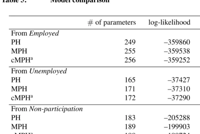
Table 5 shows the comparison of the models. Of course, extending the parameter space of a model can never decrease the likelihood. We therefore include the AIC and BIC, which both penalize the number of included parameters. The results clearly show that the multistate model has many parameters: 786 using a PH model, 810 using an MPH model and 814 using a correlated MPH model. We can conclude that the correlated MPH model is the preferred model, because it has the lowest AIC and, except for the transition from abroad, the lowest BIC.
5We also carried out formal tests on equivalence of the parameters in the PH versus MPH model and on the
Table 5: Model comparison
#of parameters log-likelihood AIC BIC
FromEmployed
PH 249 –359860 720218 722641
MPH 255 –359538 719586 722066
cMPHa 256 –359252 719016 721506
FromUnemployed
PH 165 –37427 75183 76402
MPH 171 –37310 74962 76224
cMPHa 172 –37290 74925 76195
FromNon-participation
PH 183 –205288 410942 412579
MPH 189 –199903 400184 401875
cMPHa 190 –199724 399829 401528
FromAbroad
PH 189 –25474 51326 52975
MPH 195 –25465 51321 53023
cMPHa 196 –25459 51311 53021
Notes: aCorrelated MPH.
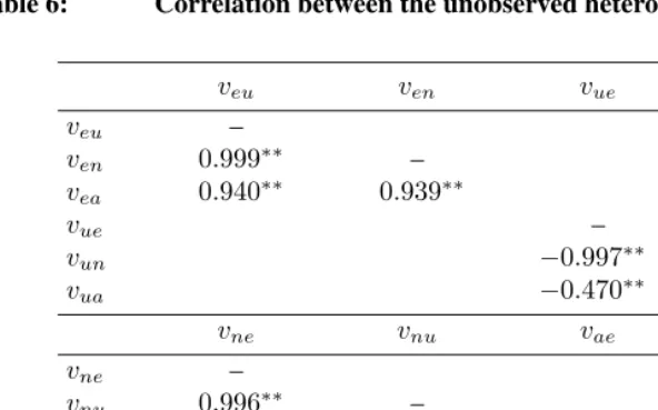
Another test on the MPH and correlated MPH models is to check the significance of the variance and the correlation. For both the uncorrelated and the correlated frailty model we find that the frailty variance is significant on a 5%-level. In the correlated model we also find significant positive correlation between the three competing frailties from the employed state, see Table 6.6This implies that employed migrants who are more
prone to become unemployed or non-participating are also more prone to leave. For each origin state we also tested whether theα’s, the factor loadings, of each factor are equal. When the factor loadings are equal it implies that a shared frailty model, which restricts the correlation to one, is sufficient. However, for all four origin states, we reject this hypothesis.
6These correlations are derived from the 2 factor loading model and the standard errors are calculated using
the delta method.
Table 6: Correlation between the unobserved heterogeneity terms
veu ven vue vun
veu –
ven 0.999∗∗ –
vea 0.940∗∗ 0.939∗∗
vue –
vun −0.997∗∗ –
vua −0.470∗∗ 0.539∗
vne vnu vae vau
vne –
vnu 0.996∗∗ –
vna −0.685∗∗ −0.735∗∗
vae –
vau 0.994∗∗
van 0.312∗ 0.214∗
Notes: ∗p <0.05and∗∗p <0.01.
These results indicate that for these data of recent labour migrants to the Netherlands it is important to include frailties and to allow these frailties to be correlated. More details on the data and on other analyses using these data on return behaviour and labour mar-ket transitions can be found in Bijwaard (2010), Bijwaard (2009), Bijwaard and Wahba (2014) and Bijwaard, Schluter, and Wahba (2014).
5.
Identification issues in multistate frailty models
see Van den Berg (2001). The most important assumptions here are that the frailty has a finite mean and we have some exogenous variation in the observed characteristics. Ridder and Woutersen (2003) show that bounding the duration dependence hazard away from 0 and∞at the start is also sufficient for nonparametric identification of the MPH model, and with this assumption the finite mean assumption can be discarded.
Honoré (1993) shows that both the frailty distribution and the duration dependence are identified with multivariate event history data under much weaker assumptions. All shared frailty models are identified without additional information, such as observed covariates or parametric assumptions about the duration dependence. Furthermore, the duration dependence may depend on observed covariates in an unspecified way, and the frailty and the observed covariates may be dependent. This identifiability property holds for a broader class of frailty models, including correlated frailty models.
A caveat of multistate data is that such data is more sensitive to censoring. With univariate event history data, many types of censoring can be captured by standard adjust-ments to the likelihood function, see Andersen et al. (1993) and Klein and Moeschberger (2003). With sequential events, either recurrent or from different types, one has to be more careful. Consider two consecutive events with timet1andt2, and where the data
are subject to right-censoring at a fixed time after the starting point or the first event. Then the moment at whicht2is right-censored is not independent fromt2itself. For example,
individuals with a large value of frailty will, on average, have a short time until the first event. As a result the time until the second event will start relatively early. This implies that the time until the second event will often be censored after a relatively longer period (or not censored at all). Thus,t2and its censoring probability are both affected by frailty.
It may also happen that the process or some of the processes are not observed from the origin. With left-censoring, not to be confused with left-truncation, the analysis is more complicated, see Heckman and Singer (1984a) and Commenges (2002). In a Markov multistate model, defined in the time since the start of the process, in which censoring is independent of previous events and uses the same time scale, the censoring issues are similar to censoring issues in univariate event history models, see Andersen et al. (1993) and Aalen, Borgan, and Gjessing (2008).
A cautionary note should be given that for all these situations, identification is only possible when the model is a correctly specified mixed proportional hazards model. It is impossible to distinguish between a misspecified proportional hazard model and a correctly specified mixed proportional hazards model, see Putter and van Houwelingen (2011) for a discussion.
6.
Summary and concluding remarks
This article has provided an overview of multistate event history models with frailty, with an emphasis on semi-Markov multistate models with a mixed proportional hazard struc-ture. The literature on this subject is continuing and growing, and with the increased computer power the complexity of the models will not discourage researchers from using them. We have shown that ignoring frailty can have a large impact on the parameters of interest for the transition hazards, the duration dependence and the effect of observed covariates on the hazard. We discuss how different correlation structures of the frailties in a multistate model can be achieved.
References
Aalen, O.O., Borgan, Ø., and Gjessing, H.K. (2008).Survival and Event History Analysis. New York: Springer-Verlag.doi:10.1007/978-0-387-68560-1.
Andersen, P.K., Borgan, Ø., Gill, R.D., and Keiding, N. (1993).Statistical Models Based on Counting Processes. New York: Springer-Verlag. doi:10.1007/978-1-4612-4348-9.
Andersen, P.K. and Gill, R.D. (1982). Cox’s regression model for counting processes: A large sample study. Annals of Statistics 10(4): 1100–1120. doi:10.1214/aos/
1176345976.
Bijwaard, G.E. (2009). Labour market status and migration dynamics. Discussion Paper No. 4530, IZA.
Bijwaard, G.E. (2010). Immigrant migration dynamics model for The Netherlands. Jour-nal of Population Economics23(4): 1213–1247. doi:10.1007/s00148-008-0228-1.
Bijwaard, G.E., Franses, P.H., and Paap, R. (2006). Modeling purchases as repeated events. Journal of Business & Economic Statistics24(4): 487–502. doi:10.1198/0735
00106000000242.
Bijwaard, G.E., Schluter, C., and Wahba, J. (2014). The impact of labour market dy-namics on the return–migration of immigrants. Review of Economics and Statistics, forthcoming.
Bijwaard, G.E. and Wahba, J. (2014). Do high-income or low-income immigrants leave faster? Journal of Development Economics108: 54–68. doi:10.1016/j.jdeveco.2014. 01.006.
Clayton, D. (1978). A model for the association in bivariate life tables and its appli-cation in epidemiological studies of familial tendency in chronic disease incidence.
Biometrika65(1): 141–151. doi:10.1093/biomet/65.1.141.
Commenges, D. (1999). Multi-state models in epidemiology.Lifetime Data Analysis5(4): 315–327.doi:10.1023/A:1009636125294.
Commenges, D. (2002). Inference for multi-state models from interval-censored data.
Statistical Methods in Medical Research11(2): 167–182.doi:10.1191/0962280202sm 279ra.
Cook, R.J. and Lawless, J.F. (2007). The Statistical Analysis of Recurrent Events. New York: Springer-Verlag.
Courgeau, D. and Lelièvre, E. (1992). Event History Analayis in Demography. Oxford: Clarendon Press.
Duchateau, L. and Janssen, P. (2008).The Frailty Model. New York: Springer-Verlag.
Duchateau, L., Janssen, P., Kezic, I., and Fortpied, C. (2003). Evolution of recurrent asthma event rate over time in frailty models. Applied Statistics 52(3): 355–363.
doi:10.1111/1467-9876.00409.
Elbers, C. and Ridder, G. (1982). True and spurious duration dependence: The identifia-bility of the proportional hazard model. Review of Economic Studies49(3): 403–409.
doi:10.2307/2297364.
Flinn, C.J. and Heckman, J.J. (1983). Are unemployment and out of the labor force behaviorally distinc labor force states? Journal of Labor Economics1(1): 28–42.
doi:10.1086/298002.
Fougère, D. and Kamionka, T. (2008). Econometrics of individual labor market transi-tions. In: Mátyás, L. and Sevestre, P. (eds.).The econometrics of panel data, Funda-mentals and recent developments in theory and practice. Princeton: Princeton Univer-sity Press: 865–905.
Govindarajulu, U.S., Lin, H., Lunetta, K.L., and D’Agostino, R.B. (2011). Frailty models: Applications to biomedical and genetic studies. Statistics in Medicine30(22): 2754– 2764.doi:10.1002/sim.4277.
Heckman, J.J. and Singer, B. (1984a). Econometric duration analysis.Journal of Econo-metrics24(1–2): 63–132.doi:10.1016/0304-4076(84)90075-7.
Heckman, J.J. and Singer, B. (1984b). The identifiability of the proportional hazard model.Review of Economic Studies51(2): 231–241. doi:10.2307/2297689.
Honoré, B.E. (1993). Identification results for duration models with multiple spells. Re-view of Economic Studies60(1): 241–246. doi:10.2307/2297821.
Hougaard, P. (2000).Analysis of Multivariate Survival Data. New York: Springer-Verlag.
doi:10.1007/978-1-4612-1304-8.
Kelly, P.J. and Lim, L.Y. (2000). Survival analysis for recurrent event data: An application to childhood infectious diseases. Statistics in Medicine19(1): 13–33. doi:10.1002/
(SICI)1097-0258(20000115)19:1<13::AID-SIM279>3.0.CO;2-5.
Klein, J.P. and Moeschberger, M.L. (2003). Survival Analysis: Techniques for Censored and Truncated Data (2nd edition). New York: Springer-Verlag.
Lancaster, T. (1979). Econometric methods for the duration of unemployment. Econo-metrica47(4): 939–956.doi:10.2307/1914140.
child survival in Malawi. Australian & New Zealand Journal of Statistics43(1): 7–16.
doi:10.1111/1467-842X.00150.
Nielsen, G.G., Gill, R.D., Andersen, P.K., and Sørensen, T.A.I. (1992). A counting pro-cess approach to maximum likelihood estimation in frailty models.Scandinavian Jour-nal of Statistics19: 25–43.
Oakes, D.A. (1992). Frailty models for multiple event times. In: Klein, J.P. and Goel, P.K. (eds.).Survival Analysis: State of the Art. Dordrecht: Kluwer: 371–379.
doi:10.1007/978-94-015-7983-4_22.
Pickles, A. and Crouchley, R. (1995). A comparison of frailty models for multivariate survival data.Statistics in Medicine14(13): 1447–1461.doi:10.1002/sim.4780141305.
Prentice, R.L., Williams, B.J., and Peterson, A.V. (1981). On the regres-sion analysis of multivariate failure time data. Biometrika 68(2): 373–379.
doi:10.1093/biomet/68.2.373.
Putter, H., Fiocco, M., and Geskus, R.B. (2007). Tutorial in biostatistics: Com-peting risks and multi-state models. Statistics in Medicine 26(11): 2389–2430.
doi:10.1002/sim.2712.
Putter, H. and van Houwelingen, H.C. (2011). Frailties in multi-state models: Are they identifiable? Do we need them? Statistics Methods in Medical Research in press.
doi:10.1177/0962280211424665.
Ridder, G. and Woutersen, T. (2003). The singularity of the efficiency bound of the mixed proportional hazard model.Econometrica71(5): 1579–1589. doi:10.1111/1468-0262.00460.
Rogers, A. (1975).Introduction to Multiregional Mathematical Demography. New York: Wiley.
Rogers, A. (1995). Multiregional Demography: Principles, Methods and Extensions. New York: Wiley.
Rondeau, V., Commenges, D., and Joly, P. (2003). Maximum penalized likelihood estimation in a gamma–frailty model. Lifetime Data Analysis 9(2): 139–153.
doi:10.1023/A:1022978802021.
Sastry, N. (1997a). Family-level clustering of childhood mortality risks in northeast Brazil. Population Studies51(3): 245–261.doi:10.1080/0032472031000150036.
Sastry, N. (1997b). A nested frailty model for survival data, with an application to the study of child survival in northeast Brazil. Journal of the American Statistical
ation92(438): 426–435. doi:10.1080/01621459.1997.10473994.
Therneau, T. and Grambsch, P. (2000). Modeling Survival Data: Extending the Cox Model. Springer-Verlag.doi:10.1007/978-1-4757-3294-8.
Van den Berg, G.J. (2001). Duration models: Specification, identification, and multiple duration. In: Heckman, J. and Leamer, E. (eds.).Handbook of Econometrics, Volume V. Amsterdam: North-Holland: 3381–3460.
Vaupel, J.W., Manton, K.G., and Stallard, E. (1979). The impact of heterogeneity in individual frailty on the dynamics of mortality. Demography 16(3): 439–454.
doi:10.2307/2061224.
Wei, L.J., Lin, D.Y., and Weissfeld, L. (1989). Regression analysis of multivariate fail-ure time data by modeling marginal distributions. Journal of the American Statistical Association84(408): 1065–1073.doi:10.1080/01621459.1989.10478873.
Wienke, A. (2011). Frailty Models in Survival Analysis. Boca Raton: Chapman & Hall/CRC.
Willekens, F.J. (1999). Life course: Models and analysis. In: Dykstra, P.A. and van Wis-sen, L.J.G. (eds.).Population Issues: An Interdisciplinary Focus. New York: Plenum Press: 23–51.doi:10.1007/978-94-011-4389-9_2.
Xue, X. and Brookmeyer, R. (1996). Bivariate frailty model for the analysis of multivari-ate survival time.Lifetime Data Analysis2(3): 277–290.doi:10.1007/BF00128978.
Yashin, A.I., Vaupel, J.W., and Iachine, I.A. (1995). Correlated individual frailty: An advantageous approach to survival analysis of bivariate data.Mathematical Population Studies5(2): 145–159. doi:10.1080/08898489509525394.
Yau, K.K.W. and McGilchrist, C.A. (1998). ML and REML estimation in survival anal-ysis with time dependent correlated frailty. Statistics in Medicine17(11): 1201–1213.