University of New Orleans University of New Orleans
ScholarWorks@UNO
ScholarWorks@UNO
University of New Orleans Theses and
Dissertations Dissertations and Theses
12-19-2008
Reconstructing Textual File Fragments Using Unsupervised
Reconstructing Textual File Fragments Using Unsupervised
Machine Learning Techniques
Machine Learning Techniques
Brian Roux
University of New Orleans
Follow this and additional works at: https://scholarworks.uno.edu/td
Recommended Citation Recommended Citation
Roux, Brian, "Reconstructing Textual File Fragments Using Unsupervised Machine Learning Techniques" (2008). University of New Orleans Theses and Dissertations. 881.
https://scholarworks.uno.edu/td/881
This Thesis is protected by copyright and/or related rights. It has been brought to you by ScholarWorks@UNO with permission from the rights-holder(s). You are free to use this Thesis in any way that is permitted by the copyright and related rights legislation that applies to your use. For other uses you need to obtain permission from the rights-holder(s) directly, unless additional rights are indicated by a Creative Commons license in the record and/or on the work itself.
Reconstructing Textual File Fragments Using Unsupervised Machine Learning Techniques
A Thesis
Submitted to the Graduate Faculty of the University of New Orleans in partial fulfillment of the requirements for the degree of
Master of Science in
Computer Science
by
Brian Roux
ii
Copyright
© 2008 Brian Roux
iii
Dedication
iv
Acknowledgement
I wish first to acknowledge my family for their continued love and support.
My thesis advisor, Dr. Golden Richard, for his advice and continued guidance.
Dr. Stephen Winters-Hilt for getting my feet wet with research and paper writing.
Dr. Vassil Roussev for his candid opinions which serve as a reminder to ignore the fluff and read all research critically.
Dr. William Greene for remembering me and sharing his experience with genetic algorithms.
Dr. Jaime Nino for his exuberance and zeal in teaching.
v
Table of Contents
List of Figures ... vii
List of Tables ... viii
Abstract ... ix
Chapter 1 ... 1
Introduction ... 1
File Carving & Fragmentation ... 1
Text Based Targets ... 2
Growing Data Size ... 2
Purpose ... 3
Organization ... 4
Chapter 2 ... 5
Background & Related Work... 5
File Carving ... 5
Information Retrieval ... 6
Document Clustering & Text Classification ... 6
Support Vector Machines (5) ... 7
Chapter 3 ... 10
Methods ... 10
Novelty & Divergence from IR ... 10
Feature Extraction ... 10
Chapter 4 ... 12
Results ... 12
Datasets ... 12
Dataset Selection ... 12
Feature Extraction ... 12
Support Vector Machine Parameters & Performance Evaluation ... 13
Preliminary Investigation ... 15
Moving to a SVM ... 17
SVM Results ... 17
Chapter 5 ... 24
vi
Unknown Tokens ... 24
RPG Dataset ... 29
Ham False Positives ... 29
Chapter 6 ... 32
Conclusion ... 32
Future Work ... 33
Works Cited ... 35
Appendix A: Creative Commons License ... 37
vii
List of Figures
Figure 1 Scholar.google.com Example of Information Retrieval ... 6
Figure 2 Hyperplane With Seperable Case ... 9
Figure 3 Hyperplane With Non-Seperable Case ... 9
Figure 4 - Sensitivity ("SN") / Specificity ("SP") Definition ... 13
Figure 5 EnableCTSRTS ... 25
Figure 6 Feldman Google Search ... 25
Figure 7 Feldman Original Website ... 26
Figure 8 Kommando Google Search ... 27
Figure 9 Fragment Frequency ... 28
Figure 10 Fragment Occurrence ... 29
Figure 11 Excerpt from copcode.txt... 30
viii
List of Tables
Table 1 FV1 Results ... 17
Table 2 FV2 Results ... 18
Table 3 FV3 Results ... 18
Table 4 FV4 Results ... 18
Table 5 FV1+2 Results ... 19
Table 6 FV1+4 Results ... 19
Table 7 FV2+4 Results ... 20
Table 8 FV1+2+4 Results ... 20
Table 9 SVM Committee Results ... 21
Table 10 .DOC Results pt 1 ... 22
Table 11 .DOC Results pt 2 ... 22
Table 12 Tertiary Fragmentation Results pt 1 ... 23
Table 13 Tertiary Fragmentation Results pt 2 ... 23
ix
Abstract
This work is an investigation into reconstructing fragmented ASCII files based on content analysis motivated by a desire to demonstrate machine learning’s applicability to Digital Forensics. Using a categorized corpus of Usenet, Bulletin Board Systems, and other assorted documents a series of experiments are conducted using machine learning techniques to train classifiers which are able to identify fragments belonging to the same original file. The primary machine learning method used is the Support Vector Machine with a variety of feature extractions to train from. Additional work is done in training committees of SVMs to boost the classification power over the individual SVMs, as well as the development of a method to tune SVM kernel parameters using a genetic algorithm. Attention is given to the applicability of Information Retrieval techniques to file fragments, as well as an analysis of textual artifacts which are not present in standard dictionaries.
1
Chapter 1
Introduction
Digital forensics is a subfield of computer science dealing primarily with the acquisition, preservation, and analysis of data from computer or computer related systems, media, and other similar sources. Part of digital forensic practice deals with acquiring data from systems damaged or compromised in some way from intentional spoliation, damage to either the physical data storage medium or logical damage to the medium’s underlying file structure (disk formatting, damage to the file table, etc), or an
inaccessible storage mechanism (either through being unknown, encrypted, or otherwise obfuscated from the investigator.) In circumstances where the information cannot be directly accessed through normal operations or interfaces digital forensic investigators must use alternative channels and tools to locate the data and make it accessible again.
The most common situation in the current landscape of digital forensics an investigator is likely to encounter is a reformatted hard drive or deleted files. Most laymen do not understand the internal mechanics of the operating system / file system at work when a file is deleted, and because of this deleted data is often still resident on the storage medium. This deleted data can be made accessible again using a forensic technique called file carving.
File Carving & Fragmentation
Many file types have invariant sections which are collectively referred to in digital forensic research as file “headers” and “footers” depending on their position at the start or end of a file respectively. By knowing these invariant bytes and their position within a given file it is possible to search through the raw data on a storage medium and identify where files of a known type start or end. Authors of modern file systems have worked diligently to minimize file fragmentation so often the files searched for are contiguous, having no fragmentation between the beginning header and ending footer; such contiguous files become easy to recover by extracting or “carving” out the contiguous data between the header and footer thus delivering the original file.
While fragmentation is minimized in modern file systems when the drives are not filled to capacity, a recent study shows some fragmentation still occurs in 6% of files present on the system. This
fragmentation is most likely to occur in cases where data is appended to an existing file and is expected to occur disproportionately in user generated files such as documents, email stores, or databases as well as system generated files such as system logs (1).
Fragmentation is a difficult problem to deal with on a generalized level because traditional approaches of file carving are intended to deal with file recovery where the complete or near complete recovery of the file is necessary for the data to be useful; for example Jpeg images where missing portions disrupt the decompression and rendering process are not useful unless the majority of the data is present. In cases where binary or media based files are the primary target of the investigation this type of
2
complex and often requires a priori knowledge of the specific file type’s internal structure for
reconstruction or validation. Prior work in this regard is discussed in the Related Work section dealing with object validation.
Text Based Targets
Data comes in two basic forms: binary, and text. When an investigation is not primarily driven by image or similar binary media based targets then the target is usually one of information or communication. As previously mentioned, a disproportionate amount of fragmentation occurs where data is appended rather than overwritten as is the case with documents, email stores, databases, system log files and other similar information containing files; in fact user generated content (which generates binary only data) is more likely to overwrite the file with a new one than append to the file (as is the case with many graphic or multimedia applications). These file types all convey textual information and communication either generated by the user and thus about the user directly (including instant message conversations, emails, spreadsheets, documents, etc), or generated by the system often about the activities the user is engaged in thusly about the user indirectly (login / logout times, accessed resources on the network or internet, etc.)
Textual data differs from its binary counterparts in that it requires no rendering or preprocessing and chunks of it, even if from only a portion of the overall file, are useful to an investigator. Because of this property textual information is paradoxically both more resilient for recovery, and more resistant to recovery where its resiliency stems from the usefulness of the fragments independent of the overall file’s recovery, and its resistance from the common lack of header or footer information for a file carving application to lock on to. While chunks of textual data are useful, it is nearly impossible to determine if a given chunk of textual data is a single fragment from one original document, or if the chunk is composed of multiple fragments contiguously stored on the medium. This indeterminate problem stems from the aforementioned lack of file headers and footers causing both cases (one chunk from an original
document, or multiple fragments from different documents in a single contiguous chunk) to be indistinguishable from the other on a structural level due to this absence.
Growing Data Size
Another problem compounding efforts in file carving techniques is the growing size of storage medium and decreasing price per gigabyte. In the course of one decade (1996-2006) hard drive size increased by over 23,437% (3.2 GB to 750GB) but rotational speed only increased by a little over 33% (5400RPM to 7200RPM) in commodity drives. Already in late 2007 / early 2008 we are seeing terabyte size drives, and multi-terabyte devices at the consumer level. This continuing increase in consumer drive size effectively makes current fragmented reconstructions infeasible for large data stores due to the exponential number of comparisons required in the recovery. Specifically, finding all other fragments which match a specific one even using an impossible classifier with perfect accuracy requires (N2)-1 comparisons if the files are, on average, bi-fragmented and (N3)-1 comparisons for tri-fragmentation, and so forth.
3
human component of the forensic investigation is the primary bottleneck. File carving techniques which must be carefully reviewed and/or generate significant false positive percentages are unduly taxing on the digital forensic investigator. Forensic tools must be designed to minimize the demand on an investigator’s time.
Purpose
I have made several assumptions about the nature of textual communication keeping in mind three axioms: (a) user or system generated data with a textual component is more likely to be appended than other sources of data, (b) appended data is disproportionately fragmented even in modern file systems which strive for minimal fragmentation, and (c) textual data is resistant to current generation file carving techniques, but resilient to total removal as even chunks of textual data independent of the complete file are usable.
First, textual communication, whether human generated or automatically generated by the system, is generated with a communicative purpose. On a generic level it is written to communicate something: a system log may show activities, and email to your family may convey information on current events in your life, or a work document may show status updates on current projects. In general the
communication is going to be concise. A document is going to tend to cover fewer (or even one) rather than many topics and documents communicating multiple topics will do so because of some relation between the topics.
Secondly, natural languages with which textual documents are written convey information through grammatical constructs of nouns, verbs, and other assorted words. These words together convey more information than an individual word would. Words and the meanings they convey form, when brought together in a document, an underlying meaning thread (“Meaning Thread”). We as humans fluent in the language the document is written in pickup on these underlying Meaning Threads as a subject.
Depending on what a document conveys it is likely to have multiple meaning threads in it. For example, a paper dealing with file carving will have an underlying meaning thread of digital forensics, file systems, files, and so forth as it deals with all of those subjects.
Thirdly, by analyzing the words and associated meanings of various documents both in comparison to parts of themselves and against other documents both related and unrelated it should be possible to differentiate between related documents and portions of the same document based on the combination of meaning threads as conveyed by word/meaning content.
4
In the course of this research and tool development I take special care in ensuring the implementation is both scalable and distributable with minimal attention or feedback required from the forensic
investigator. These two factors are essential for future forensic tool development to account for problems in growing data set size and the limited attention a forensic investigator can devote to a tool; in particular it is my opinion future tools will have to be completely automated in the near future to be of any use in forensic investigations.
Organization
In this thesis I will present results from my research into reconstructing non-contiguous fragments from ASCII text files using novel techniques drawn in a cross-disciplinary approach between Artificial
Intelligence, Information Retrieval, Digital Forensics, and other fields. In chapter 2 I will discuss
5
Chapter 2
Background & Related Work
File Carving
Computer files often contain information at the beginning or end which deals with format, length, file ending, and so forth. In many cases certain byte positions within these header and footer regions is invariant between files. These invariant header portions are often the same magic numbers used by the Linux file command to deduce file type from the header portion, but do not have to be intentional magic numbers; any byte sequence which is invariant or near invariant will do so long as it is consistent.
Current generation file carving tools use a two pass approach to carve files from raw data. In pass one they search byte by byte comparing what is found with a list of known header and footers while taking note of type and offset for each located header or footer. Using the information gleaned from pass one the file carving utility then examines headers and footers as they are positioned on disk to identify which match ups are likely to be contiguous files (such as a header for file type X followed by a footer for file type X a few blocks later.) Alternatively files can be partially recovered by reading data until an
unanticipated header or footer is encountered which does not correspond to the initial header (such as reading an image header and then later encountering a non-image header or footer.) Depending on the file type, partial recovery can be useful if the entire file is not necessary to glean some information.
The first file carving application was produced by the Defense Computer Forensics Lab in 1999 and was called CarvThis. Kris Kendall developed snarfit shortly afterward in 2001. Later both Kris Kendall and Jesse Kornblum worked together to produce Foremost. (1)
Foremost itself started as a standard file carver based on header / footer identification. In 2005 Nick Minkus published his thesis which extended foremost with several new heuristiscs including support for Object Linking and Embedding (“OLE”) file types opening up file carving to a host of Microsoft Office (“MSOffice”) files. His work modified an API package developed by the Chicago Project
(http://chicago.sourceforge.net/) to be usable by Foremost. The Chicago Project provided functionality specifically for dealing with excel files. Prior to his contribution Foremost was only able to handle Microsoft Word files. (2)
Also in 2005 Dr. Golden Richard and Dr. Vassil Roussev published Scalpel as a new file carving tool which corrected inefficiencies in the Foremost to create a much faster file carving utility. (3)
6
Information Retrieval
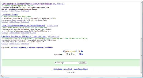
Information Retrieval (“IR”) is a cross disciplinary venture primarily concerned with searching for information pertinent to a query. The most obvious and visible IR applications are search engines such as Google and Yahoo. The primary aim of IR, arguably, is to allow an individual to rapidly winnow down a large repository of information down to documents specific to the individual’s search goals. The
information used includes not only the internal document text, but also metadata such as dates, authors, and organizations. In figure 1 we see an example of this where a simple search for file carving research also lists key authors to narrow the total search population by.
Figure 1 Scholar.google.com Example of Information Retrieval
Document Clustering & Text Classification
Document Clustering and Text Classification are subfields of IR where the primary goal is not to retrieve information by query, but to automatically put a new document into a category with other documents with related topics. An individual document may belong to multiple categories or topics which could be activated by a search query.
Term Frequency – Inverse Document Frequency (4)
Term Frequency – Inverse Document Frequency (“TFIDF”) is a statistically derived weight for how important a specific term is within a specific document modified by its pervasiveness within a document corpus. More simplistically the more often a term appears in a given document, the more important it is for classification; however, the more often a term appears in documents throughout the corpus the less important it is for classification. Therefore TFIDF is a balancing of a term’s importance to the document diminished by how commonplace it is within documents in general.
7 Where:
TF(i,j) is the Term Frequency of term i in document j is the number of occurrences for term i in document j
is the number of occurrences of all terms in document j
is the number of documents in the corpus
is the number of documents in the corpus containing term
TFIDF(i,j) is the Term Frequency – Inverse Document Frequency of term i in document j in the corpus
Cosine Similarity& Tanimoto Coefficient (4)
Cosine Similarity in a text mining / IR context refers to the similarity, expressed as an angle in the range *0,π+ with 0 denoting equivalence and π denoting complete dissimilarity. Recall the equation for expressing the dot product of two vectors in terms of the angle between them:
The cosine similarity function uses the TFIDF values as vectors for each document, and computes the angle between the TFIDF vectors as a measure of similarity for the documents being compared. The end computation to determine this similarity is as follows:
The function yielding the cosine similarity may be further extended to produce the Tanimoto coefficient which yields the Jaccard index when the input vectors are binary as follows:
The Jaccard index itself is a measure of similarity within a sample set.
Support Vector Machines (5)
8
power of this approach is greatly extended by the added modeling freedom provided by a choice of kernel. This is related to preprocessing of data to obtain feature vectors, where, for kernels, the features are now mapped to a much higher dimensional space (technically, an infinite-dimensional space in the case of the popular Gaussian Kernel).
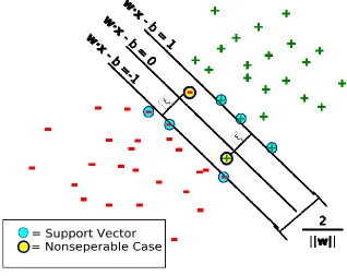
The hyperplane itself is centered at w•x – b = 0 where w is the normal vector to the separating hyperplane, x is the vector of points satisfying the above equation, and b is the offset from the origin. Given this, w and b are chosen to maximize the distance or gap between parallel hyperplanes w•x – b = -1 and w•x – b = 1. The separable case for the SVM occurs where there is no crossover from the labeled groups over the hyperplane. Non-separable cases are handled through the use of slack values (6) (see Fig. 2) to allow for some cross over in order to still obtain the largest possible margin between the bulk of the labeled groups. One of the strengths of SVMs is that the approach to handling non-separable data is almost identical to that for separable data. (8)
Upon introducing Kernels, the SVM equations are solved by eliminating w and b to arrive at the
following Lagrangian formulation: max ∑(i=1...n) αi – ½∑(i,j=1...n) αiαjyiyj K(xi,xj), subject to αi ≥ 0 and ∑(i=1...n) αiyi
= 0, where the decision function is computed as f(x) = sign(∑(i=1...n) αiyiK(xi,xj)+ b), and where K(xi,xj) is the
kernel generalization to the inner-product term, <xi,xj>, that is obtained in the standard, intuitively
9 Figure 2 Hyperplane With Seperable Case
This figure shows two clusters of labeled data which can be completely separated by a hyperplane.
Figure 3 Hyperplane With Non-Seperable Case
10
Chapter 3
Methods
In conducting my study of fragmented text documents I explored numerous methods for representing the meaning content of a given document. For most machine learning applications natural language texts such as those I am dealing with must be translated into a numerical representation for comparison against other documents. In this thesis I refer to this process as feature extraction and the resulting mathematical representations as a feature singularly or collectively as a feature vector.
Novelty & Divergence from IR
Traditional methods of Information Retrieval or Document Clustering / Text Classification rely on existing broad predefined topics for classification. In its simplest form this process can be manual such as tags in blogs, journals, or Content Management Systems, or it can be more complex in systems which automatically classify documents into existing taxonomical systems. In all cases the topic structures are self-evidently broad and intended to encompass numerous document populations for easy searching. If we were to look at this process as book classification, IR / Document Clustering would be the
classification of a new book into its correct location within the Dewey Decimal (9) system. The goal of my thesis work is to identify fragments of the same original document as they relate to each other and, viewed in a similar abstraction, this would be akin to taking chapters torn from random books and grouping them back together based on the book they originated in without the benefit of titles (headers/footers).
Feature Extraction
Numerous methods of feature extraction were evaluated in the course of this work. Because of the work’s nature approaches which in prior work were not effective for document clustering or text classification were evaluated anyway to evaluate whether the methods may have been inappropriate to document clustering due to being too specific to the document (a failure in document clustering, but a potential success in reconstructing document fragments.) In all cases the text is processed by treating non-alphanumeric characters as delineators and processing all text between the delineators as individual tokens.
Word Frequency & Natural Language Processing
11
further in cases where a one term is used more frequently at the start of a document and another in the later section reconstruction would be affected by not counting the terms similarly.
Terms which do not occur in the NLP database (or a dictionary) including misspelled words, proper names, and highly specific terms will be each referred to as a Highly Specific Term (“HST”) in the remainder of this text. HSTs offer potential for identifying characteristics of the author in cases where words are misspelled consistently, of subject where proper names are used both for people (Alice, Bob, etc) or for programs/services in log files (Apache, IIS, etc), or finally of terms with very technical or specific connotations such as those invented for use in a document.
For the Word Frequency & Natural Language Processing (“WF&NLP”) feature extraction the fragment being compared (“target”) and the files the target is compared to (“comparison”) are processed to compute the (a) Meaning Term Frequency for each NLP based meaning, (b) the standard deviation by occurrence the meaning falls into, and (c) the list of unknown tokens in the document.
TFIDF Automatic Keyword Extraction
12
Chapter 4
Results
Datasets
The experimental datasets come from the textfiles.com archive (“datastore”) which consists of over 55,000 text documents archived from Usenet, Bulletin Board Systems, and other similar sources. The data is published in hand classified categories based on topic, with sub categories relating to more specific aspects. The datastore's total size is approximately 1.2GB of ASCII text files.
Dataset 1 (“Random1”) consists of approximately 100 files selected randomly from the total datastore. Files were selected without regard to file size.
Dataset 2 (“Random2”) consists of approximately 100 files selected randomly from the total datastore. File with a total size of less than 8k were discarded from consideration.
Dataset 3 (“HamRadio”) consists of approximately 100 files selected randomly from the Ham Radio subset of the total datastore. This is a subject specific data set dealing with Ham Radio, and other related technologies and discussions. Files with a total size of less than 8k were discarded from consideration.
Dataset 4 (“RPG”) consists of approximately 100 files selected randomly from the Role Playing Games subset of the total datastore. This is a subject specific data set dealing with Role Playing Games such as Dungeons and Dragons, and similar publications.
Dataset Selection
Random2 and HamRadio were created without files smaller than 8k to more realistically simulate ondisk fragmentaiton of NTFS file systems whose default block size is 4k thus representing at minimum 2 blocks of textual data. Random1 and RPG were created without regard to this limit to evaluate differences in performance on sets using smaller datasets.
Random1 and Random2 are randomly selected datasets thus having little if any noise from fragmented documents with similar topics. These two datasets are the optimistic baseline for estimating maximum accuracy. RPG and HamRadio are subject specific datasets and serve as worst case, or pessimistic baseline for the hardest case of classification where all fragments share a topic. Further, many of the documents in RPG are game mechanics related documents which differ from standard documents such as emails, essays and so forth in that they communicate discrete sections of rules which may or not be content related.
Feature Extraction
13
SN = Or the percentage of true matches detected.
SP = Or the percentage of false positives.
Figure 4 - Sensitivity ("SN") / Specificity ("SP") Definition
Feature Vector 1 (“Cos/Tan FV”) is a magnitude 2 feature vector consisting of the Cosine Similarity, and Tanimoto coefficient. Cosine similarity is a measure of how similar two documents are with 0 denoting identical documents, and π denoting completely dissimilar documents. The Tanimoto coefficient is an extension of Cosine similarity which produces some additional data in the event of binary attributes. These two measures are well established in text mining and search engine optimization. (10)
Feature Vector 2 (“Keyword FV”) is a magnitude N feature vector consisting of a keyword comparison between the Target and Comparison files. Each document has a ranked list of keywords automatically extracted by taking the tf-idf for each term appearing in the document and selecting the N highest ranking (relevance by tf-idf weight) terms in the Target. Keyword FV is then constructed as a binary (1,0) vector with a 1 indicating the appropriate keyword from the Target fragment is present in the
Comparison fragment. N=10 was used for these experiments.
Feature Vector 3 (“Unknown FV”) is a magnitude N feature vector consisting of comparisons between the unknown tokens in the Target fragment, and those in the Comparison fragment. The comparison is similar to the Keyword FV in that it selects the N most occurring unknown tokens from the Target fragment and produces a quotient between it and the token's number of occurrences in the Comparison. N=5 was used for these experiments.
Feature Vector 4 (“Unknown Ratio FV”) is a magnitude 1 feature vector consisting of a ratio between the number of unknown tokens the two fragments have in common and the total number of unknown tokens in the Target fragment.
Support Vector Machine Parameters & Performance Evaluation
The primary mechanism altering effectiveness of the SVM is the selection of a kernel which performs well for the feature vectors being studied, as well as a set of parameters for the selected kernel which are stable for the feature vectors. The general aim for kernel and parameter selection is to maximize accuracy where accuracy = (SN + SP) / 2. Due to the nature of fragment reconstruction, the number of correct combinations is far outnumbered by incorrect combinations. For example, 100 files split into 200 fragments have N*(N-1) comparisons which works out to 200 * (200-1) = 200 * 199 = 39,800 total comparisons of which there are 2N-1 correct combinations (Fragment A matched with Fragment B, and Fragment B matched with Fragment A) giving 2*200-1 or 399 correct combinations, and 39,800 – 400 = 39,401 incorrect combinations. The aim of automated digital forensic tools is to lessen the workload of a human analyst, so an increase in SN at the expense of a decrease in SP becomes self defeating as the erroneous classifications drown out the correct reconstructions. In perspective, 30% SN with 99.9% SP would involve the identification of approximately 119 correct reconstructions and 39 incorrect
14
0.5% decrease in SP there would be a total of approximately 160 correct reconstructions, and 236 incorrect reconstructions increasing the manual review process to almost 1% of the total brute force work. Following from this, anything under 99% SP quickly becomes untenable as the noise drowns out any correct reconstructions.
Current practice in SVM usage is to perform kernel selection and parameter tuning through a repeated retraining process in an attempt to find a kernel which has a good general performance for the feature vector, and kernel parameters which provide stable performance. Stable performance, as referred to here, is defined as performance for which minor modifications of a kernel parameter have a
performance change proportional to the change in the kernel parameter e.g. minor changes in a kernel parameter yield minor changes in performance. Conversely, unstable performance occurs where minor changes in a kernel parameter result in erratic or disproportionate changes in performance results. This process can be quite tedious, and requires the user to hand select parameters. Because the
effectiveness of a kernel and its parameters can be easily and accurately evaluated against a given training and testing data set the overall problem screams for the application of a genetic algorithm to automatically tune the kernel parameters in finding the most effective settings for the training and classification process. To this end a prototype SVM auto-tuning genetic algorithm was applied in the training process:
Step 1: Initial Population – A given kernel is selected for testing and an initial population of parameters is randomly generated. For these experiments a population size of 50 was chosen.
Step 2: Evaluation & Selection – Given two datasets (training and testing) each member of the kernel population is used to train an SVM, and then classify the testing set. The genetic
algorithm evaluation function uses the exact measures of SN and SP to determine success of the member, and the average performance of the population is computed. A cut off point is set midway between the average and best performance in the population with members falling below the cut off selected for extinction and those above or at it allowed to breed.
Step 3: Breeding – The surviving members of the current generation are preserved in the next, and are randomly bred with each other to refill the population to its maximum level. Again, for these experiments maximum population is set at 50. When two members are bred, their parameters are blended by averaging between the parents.
Step 4: Mutation – Mutate a portion of the population to have their parameters randomly mutated by + or – 1 for integer parameters, or a decimal in the [0,1) range for double parameters. For this application 10% of the population was selected for mutation at each generation.
Repeat 2-4 until the population becomes homogeneous or performance gains cease or become negligible (bellow a threshold value.) The final generation contains the best performing
15
The method of breeding chosen (averaging the kernel parameters) causes breeding to perform an exaggerated form of hill climbing akin to a binary search. Specifically given two well performing points A and E will breed to average out to C, a mid point, in the next generation. Depending on the performance at the three points, in successive generations a survival of A and C will breed to produce B while
alternatively E and C will produce D. This behavior diverges from a binary search though in that
performance is not a linear increase coupled to kernel parameter, instead there are peaks and valleys in performance so points B and D could both be well performing values better than their ancestors A, C, and E. The random mutation aspect also serves to knock out unstable regions where a single value performs well for the specific data set, but doesn’t have a generally good performance over similar data sets in that along the way. For example if the specific B performs well, but B ±0.000001 performs badly, then B is not a good value to use; in such a case the “jittering” of the parameter through mutation will help knock the population out of such an oddity. If the jittered value performs well, but not quite as well as the original it will eventually find its way back through successive breeding. The end result of a good run with this method of auto tuning is a range of kernel parameters with a similar performance, where the parameters are numerically close.
Kernel selection is not the sole determinant for SVM performance; the feature vectors themselves are equally important to the success of learning. Rerunning a genetic algorithm for near optimal
performance is unnecessary to evaluate whether the addition of alternative features to the feature vector could increase performance. For a given set of kernel parameters with stable performance, the change in performance with the addition of new features can be used to determine if they should be included without requiring the kernel parameters to be tuned. Once additional features are evaluated as increasing the performance of a SVM the augmented feature vectors can be tuned with the genetic algorithm without expending the computational resources and time to tune for each considered feature addition. More simply, we only tune for near optimal performance on additional features which are shown to provide a benefit and discard those features which provide no appreciable benefit. For these experiments the radial kernel with gamma = 2 was selected as it has previously been observed as a generally well performing kernel to evaluate addition or subtraction of features in prior unrelated work. (5) Though gamma = 2 is a stable kernel parameter used for much of the early work, once the auto-tuning SVM algorithm was introduced a significant performance increase was obtained as detailed in the results section.
Preliminary Investigation
A preliminary investigation was conducted into the problem under the assumption NLP information could be used to deduce an underlying set of topics from a document based on extracting and
16
information in quantity; i.e. an apache log will contain data relating to an apache process, and use some terminology specific to apache log files or web servers.
Most human readable documents convey information in a discrete manner dealing with a single topic thread or subject. Longer documents will tend to have broader subjects to deal with while shorter ones will tend towards being concise.
The pervasive meaning thread in a document is conveyed by words, but there are many words in a language to describe the same meaning. Half of a paper on dogs may use the word “dog” while the second half could favor “canine” if shifting focus, but the meaning throughout refers to the same subject. NLP provides a way to map dissimilar words to a common meaning through databases which map the relationships words have to each other.
It was initially assumed fragments of the same document should have similar frequencies of common meanings since they 1) deal with the same subject, 2) are part of the same document, and 3) have a common writing flow. Therefore, it was further assumed analyzing the common meaning and their frequency in one fragment as compared to another should allow fragments to be clustered into the documents they came from.
The NLP Ratio FV was originally derived from this approach, and in the course of preprocessing the documents' terms into NLP meanings the idea to target unknown tokens was adopted shortly after. The unknown tokens themselves were compared as a simple ratio of occurrences which became the
Unknown Ratio FV. Prior to the adoption of the SVM as the preferred learning method, very small datasets were compared using the J4.8 decision tree algorithm. The input data consisted of the NLP Ratio FV, and the Unknown Ratio FV expressed for both possible comparisons (e.g. with FileA as the Target and FileB as the comparison, and vice versa.)
17
Moving to a SVM
Increasing the training size did not give any significant increase in performance from the decision tree classifier so the experiments were moved to SVM based learning. In the process more research was examined into document clustering techniques. The problem of fragment reconstruction has some similarities to Information Retrieval in that some topic common between the two fragments is sought in a similar way to document clustering where some topic common between two documents is sought. The complication in identifying two fragments from the same document is many fold: First, to somehow identify a difference between fragments of the same source, and fragments of different documents of the same category. Second, to make the resulting classifier general to any document. Third, to increase SN to a point where the process is useful to a forensic analyst but keeping SP high enough so that the useful information is not drowned out by the noise.
The overarching theme here can be summarized as detecting the similarities between the fragments as well as the differences between the document and other similar documents. Detecting that fragments of a pie recipe are different from a tutorial on poker is significantly easier than detecting fragments of a peach pie recipe are from a fragment of another recipe for peach cobbler, and detecting the differences between two peach pie recipes may be nigh impossible.
The Cos/Tan FV consists of two measures, Cosine Similarity and Tanimoto Coefficient, commonly used in Information Retrieval for measuring document similarity with the Tanimoto Coefficient being a variation of the Cosine Similarity. This feature vector was lifted directly from common Information Retrieval techniques. Similarly, the Keyword FV was derived from Term Frequency – Inverse Document Frequency (“tf-idf”), another common technique for IR, with the tf-idf used in such a way to extrapolate, unsupervised, a list of the N most important keywords in a document and compare them as previously described to another document.
The datasets as previously described were processed to produce the feature vectors also previously defined. These feature vectors were then evaluated on their own, and in combination to determine effectiveness. Afterward, the promising combinations were put through an automatic tuning process using the aforementioned genetic algorithm to determine the parameters needed for near optimal performance. The results from this process are presented below.
SVM Results
Individual Feature Vector Results
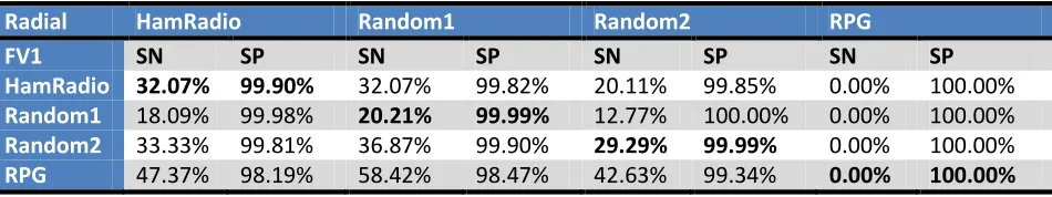
Radial HamRadio Random1 Random2 RPG
FV1 SN SP SN SP SN SP SN SP
18
Table 1 summarizes results from FV1 consisting of the Cosine Similarity and Tanimoto coefficient of two compared fragments. Initial results here are from the Radial kernel operating with Epsilon 0.02, Gamma = 2.67812144546692 and C = 1. This classifier is running at an average SN of 23.95% with a 99.70% SP translating into almost ¼ of the fragments being correctly grouped into the original document, and only a 0.30% false positive rate on all possible comparisons. Of specific note is the abysmal performance on the RPG set. Even with an inability for RPG to converge, however, it still has some strong classification power on the other data sets.
Radial HamRadio Random1 Random2 RPG
FV2 SN SP SN SP SN SP SN SP
HamRadio 14.13% 99.98% 23.37% 99.29% 41.30% 98.61% 11.96% 99.82% Random1 5.32% 99.99% 30.85% 99.98% 26.60% 99.78% 7.98% 100.00% Random2 8.59% 99.99% 27.78% 99.85% 28.79% 99.98% 9.09% 99.96% RPG 3.68% 99.91% 22.11% 99.70% 34.21% 99.28% 22.63% 99.96% Table 2 FV2 Results
Table 2 FV2 Results summarizes results from FV2 consisting of a keyword comparison between the Target and Comparison files. Initial results here are from the Radial kernel operating with Epsilon 0.02, Gamma = 2 and C = 1. This classifier is running at an average SN of 19.90% with a 99.75% SP.
Radial HamRadio Random1 Random2 RPG
FV3 SN SP SN SP SN SP SN SP
HamRadio 0.00% 100.00% 0.00% 100.00% 0.00% 100.00% 0.00% 100.00% Random1 0.00% 100.00% 0.00% 100.00% 0.00% 100.00% 0.00% 100.00% Random2 0.00% 100.00% 0.00% 100.00% 0.00% 100.00% 0.00% 100.00% RPG 0.00% 100.00% 0.00% 100.00% 0.00% 100.00% 0.00% 100.00% Table 3 FV3 Results
As seen from Table 3 FV3 Results, FV3 (the presence or absence of the top N occurring unknown tokens of the target fragment in the comparison fragment) performance was an across the board failure. Unlike the results about to be presented for FV4, FV3 had no additional classification power when combined with other feature vectors. Possible reasons for this occurrence will be explored in chapter 5 under deeper analysis in the unknown token subsection. As will be explored later the probable reason for this failure in what otherwise seems to be an information rich data source may be explained by a significant amount of noise which will require filtering before FV 3 becomes viable as a classification mechanism in future work.
Radial HamRadio Random1 Random2 RPG
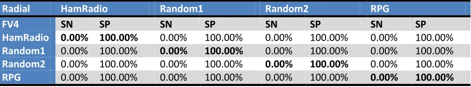
FV4 SN SP SN SP SN SP SN SP
19
Table 4 FV4 Results summarizes results from FV4 consisting of a ratio between the number of unknown tokens the two fragments have in common and the total number of unknown tokens in the Target fragment . Performance on FV4 is on first inspection a complete failure. However, as will be shown later, there is information content in FV4 but either not enough or the FV magnitude is too small to classify with an SVM. Later examples with combination feature vectors show a marked increase in SN power when FV4 is combined with one of the other FVs.
FV1 and FV2 have very similar performance; performance for both is around 20% for SN, and at or above 99.70% for SP. Each has slight variations in performance seemingly indicative of weaknesses or strengths with certain kinds of dataset comparisons such as random to subject specific, or vice versa. Moving forward, the next section examines performance gains or losses for combinations of the simple feature vectors. Henceforth analysis will concentrate on the three most effective feature vectors: FV1, FV2, and FV4.
Combination Feature Vectors Results
Radial HamRadio Random1 Random2 RPG
FV1+2 SN SP SN SP SN SP SN SP
HamRadio 39.67% 99.97% 14.67% 99.70% 26.63% 99.77% 1.63% 99.99% Random1 10.64% 100.00% 50.00% 99.96% 16.49% 99.97% 4.26% 100.00% Random2 19.70% 99.91% 33.84% 99.82% 61.62% 99.99% 10.61% 99.99% RPG 16.32% 99.33% 23.68% 99.35% 31.58% 99.47% 42.11% 99.99% Table 5 FV1+2 Results
Table 5 FV1+2 Results summarizes the results from Combination Feature Vector (“CFV”) FV1+2 (a feature vector formed by combining FV1 and FV2.) FV1 and FV2 yielded an average SN of 23.95% and 19.90% respectively, the combined vector FV1+2 raised the average SN to 25.21% for a performance gain of 1.26-5.31% with an increase to SP versus FV2 of 0.08% and a decrease to SP versus FV1 of 0.13%. Initial results here are from the Radial kernel operating with Epsilon 0.02, Gamma = 1.340775 and C = 1.
Radial HamRadio Random1 Random2 RPG
FV1+4 SN SP SN SP SN SP SN SP
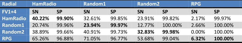
HamRadio 40.22% 99.90% 32.61% 99.85% 23.91% 99.82% 2.17% 99.97% Random1 20.74% 99.96% 23.94% 99.97% 12.77% 100.00% 2.66% 100.00% Random2 38.89% 99.66% 40.91% 99.73% 32.83% 99.98% 0.00% 100.00% RPG 65.26% 96.88% 71.05% 96.77% 53.68% 99.04% 6.32% 100.00% Table 6 FV1+4 Results
Table 6 FV1+4 Results summarizes the results from FV1+4 a CFV combining FV1 and FV4. FV4 yielded an average SN of 0% making a comparison to FV1+4 irrelevant and a SN increase of 9.35% over the
20
has enough to push the gray area back or the addition of the FV4 components to the FV1+4 vector open up a clearer separating hyperplane within the dataset. Initial results here are from the Radial kernel operating with Epsilon 0.02, Gamma = 1.08855013343707 and C = 1.
Radial HamRadio Random1 Random2 RPG
FV2+4 SN SP SN SP SN SP SN SP
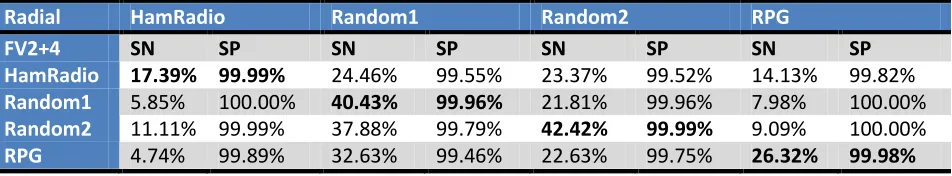
HamRadio 17.39% 99.99% 24.46% 99.55% 23.37% 99.52% 14.13% 99.82% Random1 5.85% 100.00% 40.43% 99.96% 21.81% 99.96% 7.98% 100.00% Random2 11.11% 99.99% 37.88% 99.79% 42.42% 99.99% 9.09% 100.00% RPG 4.74% 99.89% 32.63% 99.46% 22.63% 99.75% 26.32% 99.98% Table 7 FV2+4 Results
Table 7 FV2+4 Results summarizes the results from FV2+4 a CFV combining FV2 and FV4. Of this group of CFVs formed from two individual feature vectors, the FV2+4 group is the worst performing. It provides an SN increase of 1.49% SN over FV2 alone. Again here, while modest, the addition of the previously badly performing FV4 to the FV2 results in a performance increase. Initial results here are from the Radial kernel operating with Epsilon 0.02, Gamma = 0.19601 and C = 1.
The next stage was to continue the path of combining the FVs to squeeze out additional performance.
Radial HamRadio Random1 Random2 RPG
FV1+2+4 SN SP SN SP SN SP SN SP
HamRadio 42.93% 99.98% 11.41% 99.91% 15.22% 99.90% 2.17% 99.99% Random1 10.11% 100.00% 51.60% 99.99% 15.43% 99.99% 1.60% 100.00% Random2 15.66% 99.93% 28.28% 99.88% 64.65% 99.99% 5.05% 100.00% RPG 19.47% 98.81% 16.84% 99.56% 24.74% 99.48% 20.53% 100.00% Table 8 FV1+2+4 Results
Table 8 FV1+2+4 Results summarizes the results from FV1+2+4 a CFV combining all three of the simple feature vectors under consideration. SN increase was slightly over the FV2+4 CFV, but underperforming against FV1+2 and FV1+4. Initial results here are from the Radial kernel operating with Epsilon 0.02, Gamma = 0.5167 and C = 1.
Summary of Combination Feature Vectors
It is clear from the previous results the combination of individual feature vectors does provide an increase in performance, but the performance increase is not as substantial as was hoped for. All results in the previous two sections were first evaluated on the previously explained default gamma value of 2 then, as discussed, tuned using a genetic algorithm to determine a more optimal setting for the kernel function with the tuned results presented above. These will be considered optimal or as near optimal as practical for the remainder of this text.
Committee of SVMs
21
separation point between the true and false comparisons. In this next set of experiments SVMs trained on each individual feature vector are used to generate a new training set based on their classification which will in turn train a “higher order” SVM functioning similarly to a committee style classifier such as is often used with neural networks and SVMs (13).
This committee approach differs somewhat from classic committees which produce their decisions based on simple voting, or weighted voting methodologies. Here, instead, the classifications from the individual SVMs for the above IFV and CFV sets were extracted as features in a new feature vector and retrained into a Committee. It, in turn, was tuned by genetic algorithm and used as a classifier. For this experiment each individual feature vector and combination feature vector (FV1, FV2, FV1+2, FV1+4, FV2+4, FV1+2+4) is classified and the resulting classifications are used to form a new magnitude 6 feature vector. The more optimal gamma values previously determined using the automatic tuning genetic algorithm are used for the respective feature vector it performed well for.
Specifically given SVMs trained on data sets FV1, FV2, FV1+2, FV1+4, FV2+4, and FV1+2+4 the training set was reclassified to produce the functional values for each vector. (FV3, and FV4 were omitted as they had no classification power on their own, and FV3 was not used in combination with other FVs due to its lack of “bosting” power) Normally the functional value’s sign is used to determine classification (±1), but here the functional values for the comparison (Fragment A compared to Fragment B) for the 6 trained SVMs is fed into another “committee” training set, with the committee SVM trained from it. The process is repeated on testing data with the test set first classified by the individual SVMs, then the functional values combined to create a vector for the committee SVM to classify.
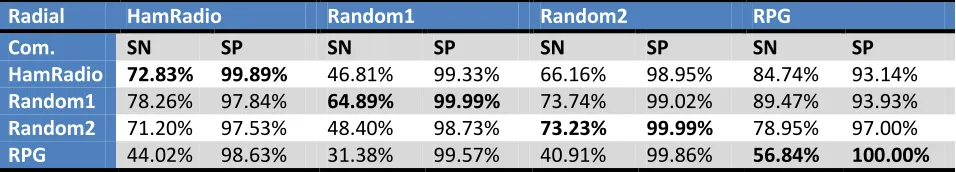
Radial HamRadio Random1 Random2 RPG
Com. SN SP SN SP SN SP SN SP
HamRadio 72.83% 99.89% 46.81% 99.33% 66.16% 98.95% 84.74% 93.14% Random1 78.26% 97.84% 64.89% 99.99% 73.74% 99.02% 89.47% 93.93% Random2 71.20% 97.53% 48.40% 98.73% 73.23% 99.99% 78.95% 97.00% RPG 44.02% 98.63% 31.38% 99.57% 40.91% 99.86% 56.84% 100.00% Table 9 SVM Committee Results
Table 9 SVM Committee Results summarizes results from the committee approach. The data shows a significant gain for training maximum SN, as well as a significant gain for testing SN with a small decrease in SP performance for testing sets. This approach over all allows the trade off of small SP decreases for large SN increases. In many cases 1-2% of SP degradation is matched by a 40-50% SN gain. Clearly the SVM applied in a committee fashion is able to use weaker information from the member SVMs which did not quite push a specific test case over the threshold and use it to deduce a positive classification from a weaker signal in effect taking advantage of multiple separating hyperplanes. Initial results here are from the Radial kernel operating with Epsilon 0.02, Gamma = 0.2089679855192752 and C = 1.
Non-ASCII Files
ASCII files are common in a system for numerous purposes of interest including log files, instant
22
interesting target for forensic examiners is the .doc file or another equivalent. These word processing files have supplanted text files as the preferred format for reports, memos, and other information sources.
A collection of 74 .doc files were gathered randomly from the Internet using Google. They were split in half based on byte count, and then the linux strings program was used to extract ASCII data from each fragment. The amount of ASCII data extractable from documents is only due to increase in the future with the shift of various popular document formats to XML rather than binary based files, and other non-word processing files such as PDF often also store ASCII data from an OCR process to allow document searches. (14)
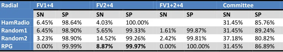
Radial FV1 FV2 FV4 FV1+2
SN SP SN SP SN SP SN SP
HamRadio 5.64% 98.34% 6.45% 99.96% 0.00% 100.00% 1.61% 99.76% Random1 8.06% 97.80% 10.48% 98.64% 0.00% 100.00% 6.45% 99.41% Random2 4.84% 98.11% 26.61% 93.29% 0.00% 100.00% 4.84% 99.36% RPG 0.00% 100.00% 5.65% 99.93% 0.00% 100.00% 1.61% 99.96% Table 10 .DOC Results pt 1
Radial FV1+4 FV2+4 FV1+2+4 Committee
SN SP SN SP SN SP SN SP
HamRadio 6.45% 98.64% 4.03% 100.00% 31.45% 85.76%
Random1 6.45% 98.90% 5.65% 99.33% 1.61% 99.87% 31.45% 89.24% Random2 3.23% 98.90% 14.52% 99.26% 2.42% 99.81% 37.18% 80.82% RPG 0.00% 99.99% 8.87% 99.97% 0.00% 100.00% 31.45% 86.89% Table 11 .DOC Results pt 2
Table 10 .DOC Results pt 1 and Table 11 .DOC Results pt 2 summarize the results from the classification process. For comparison the HamRadio and Random1 datasets were used as training sets to classify the .doc set for each of the eight feature vector sets (FV1, FV2, FV4, FV1+2, FV1+4, FV2+4, FV1+2+4, and Committee of SVMs.) Results across the board were in the 50-60% range, with most near 54% for SN, and most SP performance near 98-99%. Performance is on par with a pure ASCII file format making the approaches previously presented for ASCII files directly applicable to non-ASCII files which contain string data.
Higher Fragmentation
Previous work in the area of file carving has identified documents which are often appended as
23
performance, while necessarily degraded due to reduced information to draw on as fragment size decreases, must still be able to perform a proportionally effective classification.
To test this, the previous HamRadio sample was divided into three parts rather than two as in the earlier results. HamRadio was chosen in particular as well representative of standard prose, as well as being subject specific and thusly difficult to classify by pure subject specific words.
3 Frag FV1 FV2 FV4 FV1+2
Train/Test SN SP SN SP SN SP SN SP
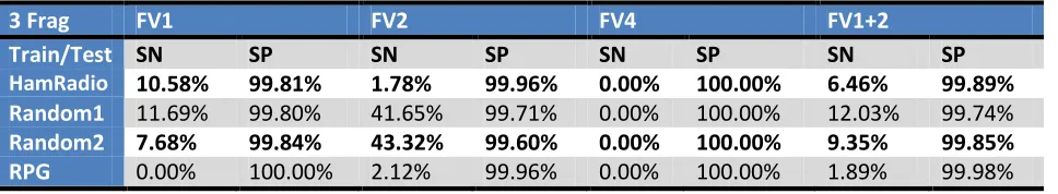
HamRadio 10.58% 99.81% 1.78% 99.96% 0.00% 100.00% 6.46% 99.89% Random1 11.69% 99.80% 41.65% 99.71% 0.00% 100.00% 12.03% 99.74% Random2 7.68% 99.84% 43.32% 99.60% 0.00% 100.00% 9.35% 99.85% RPG 0.00% 100.00% 2.12% 99.96% 0.00% 100.00% 1.89% 99.98% Table 12 Tertiary Fragmentation Results pt 1
FV1+4 FV2+4 FV1+2+4 Committee
SN SP SN SP SN SP SN SP
HamRadio 11.36% 99.87% 2.67% 99.95% 4.01% 99.93% 29.18% 99.35% Random1 10.25% 99.87% 11.47% 99.83% 9.58% 99.84% 66.37% 98.96% Random2 5.90% 99.91% 7.68% 99.88% 7.57% 99.90% 58.57% 99.02% RPG 0.56% 100.00% 1.45% 99.99% 0.89% 99.99% 14.14% 99.65% Table 13 Tertiary Fragmentation Results pt 2
24
Chapter 5
Deeper Analysis
Unknown Tokens
For the following analysis the unknown tokens for the Random2 data set were used. In the 200 fragments there were a total of over 18k unknown tokens. The early experimental work concentrated on determining a ratio between total unknown tokens in a fragment and the number it shared in
common with a comparison fragment. These results, as previously demonstrated, were not as successful as was hoped for in expanding results through SVM classifiers. However, there still appears to be
significant classification potential within the unknown token sets.
File 1 File 2 Unknown Token
promodem.txt.00 promodem.txt.01 enablectsrts
pcgpe10.txt.00 pcgpe10.txt.00 feldman
p123.txt.00 p123.txt.01 endor
Bangsonic-1.7.00 Bangsonic-1.7.01 frankie
area709doc.phk.00 area709doc.phk.01 grbank
DLPH05_25.txt.00 DLPH05_25.txt.01 johnreed
kfyi-593.hac.00 kfyi-593.hac.01 kommando
rzr1292.nfo.01 solar.nfo.01 hoppermania
aspbb4.lst.00 pcgpe10.txt.00 hillcrest
Gmj46.d70.00 govtbbs.phk.01 kimberly
jonsj2.txt.00 blooprs1.asc.00 magna
fido1102.nws.01 rrr199402.txt.00 netware
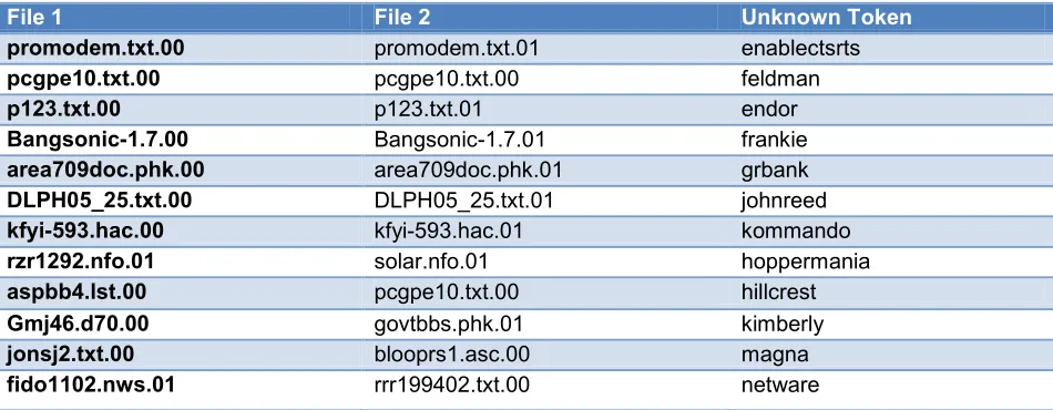
Table 14 Unknown Token Sample
Table 14 Unknown Token Sample shows a selection of unknown tokens contained in exactly two fragments in the Random2 dataset. This example shows 7 tokens where the value existed only in both fragments of the same original document and 5 tokens where the value exists in fragments of different original documents.
Promodem.txt contains the token enablectsrts in both fragments of the original document. It turns out the token is a function call EnableCTSRTS for the ProModem RS232 Interrupt Driven Serial
25 Figure 5 EnableCTSRTS
pcgpe10.txt contains the word feldman in both fragments of the original document. The document in question is entitled THE PC GAMES PROGRAMMERS ENCYCLOPEDIA 1.0 (“PCGPE”) whose author, upon cursory inspection, appears to be Mark Feldman. His name appears in several segments of the file as an author annotation to source code snippets. Again using Google to identify any other relevance as a search term the unknown token might have, the second search result yields the original home of PCGPE along with information it was discontinued in September 2000 after 3 years without updates.
26 Figure 7 Feldman Original Website
P123.txt contains the unknown token endor in both fragments of the original document. This match surprised me as I was expecting something related to Star Wars and Ewoks as Endor is more commonly associated with the Star Wars movie franchise. To my surprise the text is in fact a text on the early childhood of Jesus, and Endor is listed as one of the places Joseph worked. Google search, naturally, brings up Ewoks rather than Jesus.
Bangsonic-1.7 contains the unknown token frankie in both fragments of the original document. This document is actually a Usenet posting from alt.rec.music.comp of an “E-mag” and the token in question is picked up in both fragments as one of the contributing authors' names “Frankie Machine.”
Area709doc.phk contains the unknown token grbank in both fragments of the original document. This document is a listing of telephone exchanges in Newfoundland as of December 1991. The token in question is an index abbreviation used to denote which portions of the 709 area code its corresponding municipalities belong to. The tail end of the second fragment shows the token corresponds to “Grand Bank.”
DLPH05_25.txt contains the unknown token johnreed in both fragments of the original document. It is interesting because it occurs more than once for what prior to inspection seems a typographic error. Upon inspection the document appears to be an archive of BBS postings in which John Reed was taking part. The system displayed user names presumably based on email addresses and in the case of John Reed displayed him as JOHNREED thus dispelling the assumption as to its nature.
27 Figure 8 Kommando Google Search
The previous seven examples demonstrated unknown tokens with a high degree of classification value within the data set. Within the limited dataset examined, Random2, each would have had enough classification power to correctly classify the two fragments in and of itself, but this is unlikely to be the case in larger scale datasets. Still, the results so far are optimistic for the power of unknown tokens despite the lack luster performance in the SVM experiments. Next I analyze five instances where the unknown token is present in two fragments from different original documents.
Both rzr1292.nfo fragment 2, and solar.nfo fragment 2 contain the unknown token hoppermania. The original location of the two fragments reveals they were randomly selected from the same subsection of the archive piracy/RAZOR. The fragments appear to be identification sections of information files which would accompany pirated software distributions (“warez”). The token Hoppermania appears to be the alias for a member of the group who administrated one of the warez group RAZOR 1911 (“razor”)'s BBSes. As an interesting side note the razor group membership dynamics can be observed by comparing hoppermania's listing as an “outpost” (likely a denotation of rank or acceptance within the group) in the time of rzr1292.nfo's posting for the game Legends of Valour in December 1992, and solar.nfo's posting for the game Solar Winds: Episodes 1&2 in March 1993 where hoppermania's BBS was upgraded to an “affiliate.”
Both aspbb4.lst fragment 1 and pcgpe10.txt fragment 1 contain the unknown token hillcrest. Aspbb.lst is from an Association of Shareware Professionals BBS listing (“A.C.S. BBS”), and pcgpe10.txt is as previously discussed. In this case Hillcrest is a street name in the former, and a city in the later, both used as part of an address though the addresses themselves are unrelated.
Both gmj46.d70 fragment 1 and govtbbs.phk fragment 2 contain the unknown token kimberly.
28
Both jonsj2.txt fragment 1 and blooprs1.asc fragment 1 contain the unknown token magna. As a side note Magna is not truely an unknown token unless one concentrates only on English language
information, it is actually the latin adjective magnus, magna, magnum meaning great, or large. Jonsj2.txt is from the archive subsection on erotica stories in which one of the characters is described as
graduating magna cum laude whereas the second document blooprs1.asc is a text from the humor subsection mentioning the Magna Carta.
Finally, both fido1102.nws fragment 2 and rrr1994002.txt fragment 1 contain the unknown token netware. Netware in this example belongs the the unknown token category of highly specific terms. The former fragment contains a short passage on AT&T selling Unix to Novell in which Novell's production of Netware is identified, and the later contains another passage on the release of Dr. Dos 7 containing a version of Netware.
The twelve examples demonstrated here show a small glimpse into the possible reasons an unknown token may exist within a document as well as the classification power they may have from the highly relevant ones such as EnableCTSRTS to the near irrelevant Magna. The examples were pulled only from those tokens matched in only two fragments. Next I will examine the statistical distribution of unknown tokens by the number of fragments they occur in.
Figure 9 Fragment Frequency
As can be seen above the significant bulk of unknown tokens exist in a single fragment (roughly 13.6k of 18.4k or 74%). Contrary to my initial hypothesis, the bulk of misspelled words exist in the 74% of unknown tokens which exist in only one fragment. This thus eliminates any classification power a misspelling may have if it is not misspelled consistently and pervasively within the document. This bulk also supports the idea unknown tokens do have significant classification potential in the face of lack luster results from the SVM experiments in that the bulk of possible comparisons between fragments will be specific to only one and will drown out classification potential of the intersecting unknown tokens through sheer number. The future work section details additional steps to be taken in
0 2000 4000 6000 8000 10000 12000 14000 16000
29
investigating this phenomenon, but significant work on filtering will be required before unknown tokens can be applied with precision.
Figure 10 Fragment Occurrence
Figure 10 Fragment Occurrence is a chart detailing distribution by Occurrence. The Y axis denotes the number times an individual fragment has a token occurring a number of times specified by the X axis. As expected from Figure {Distribution Chart} the single occurrence of a token within a fragment is the majority case, and while there is no direct overlaps the curve decrease is relatively similar to Figure {Distribution Chart}. By comparing Figure {Distribution Chart} and Figure {Occurrence Distribution Chart} the populations of tokens with 2-5 occurrences which occur in 2-7 fragments seem to be the most interesting for further study. These numbers are, of course, subject to change with larger data sets under consideration.
RPG Dataset
Ham False Positives
When dealing with false positives the inherent question is: why do some files classify as positive. In some cases it is a simple inescapable aspect of inseparable cases (see Figure 3 Hyperplane With Non-Seperable Case) where the positive and negative data points overlap in some way. In other cases it is because the data files are extremely similar as in the following examples from the Ham false positives.
0 5000 10000 15000 20000 25000 30000
30
First is fragment 1 from cbbook.txt and fragment 1 from copcode.txt. When manually inspected it is obvious these two files not only deal with the same topic, Ham Radio, but with a very specific subject matter: radio codes. The specific subject is so specific in this case, the files contain almost identical sections of information:
10-0 Exercise great caution. 10-1 Reception is poor. 10-2 Reception is good. 10-3 Stop transmitting. 10-4 Message received. 10-5 Relay message. 10-6 Change channel.
10-7 Out of service/unavailable for assignment. 10-7A Out of service at home.
10-7B Out of service - personal. 10-7od Out of service - off duty
10-8 In service/available for assignment. 10-9 Repeat last transmission.
10-10 Off duty.
10-10A Off duty at home. 10-11 Identify this frequency.
10-12 Visitors are present (be discrete). 10-13 Advise weather and road conditions. 10-14 Citizen holding suspect.
10-15 Prisoner in custody. 10-16 Pick up prisoner. 10-17 Request for gasoline. 10-18 Equipment exchange.
10-19 Return/returning to the station. 10-20 Location?
Figure 11 Excerpt from copcode.txt
10-1 Receiving poorly. 10-2 Receiving well. 10-3 Stop transmitting. 10-4 OK, message received. 10-5 Relay message. 10-6 Busy, stand by.
10-7 Out of service, leaving air, not working. 10-8 In service, subject to call, working well. 10-9 Repeat message.
10-10 Transmission completed, standing by. 10-11 Talking too fast.
10-12 Visitors present.
31 10-18 Anything for us?
10-19 Nothing for you, return to base. 10-20 Location; My location is __________. Figure 12 Excerpt from cbbook.txt
What is easy to see here is the unknown tokens, which have been shown as the more powerful classifier, as well as the various similarity functions are going to pick up not only the matching 10-0 etc codes, but similar word usages within the document as a whole because essentially the two fragments, while not coming from the same document, are effectively the same.
In a similar vein other fragments such as fragment 2 of epfreq.txt have false matches to many fragments (around 10) for similar reasons. In this case epfreq.txt contains lists of radio frequencies with which government or other agency it is assigned to, and so do the fragments it matches too. Despite the name differences, these lists could be different versions of the same file.