Desert 23-1 (2018) 107-121
Spatio-temporal analysis of diurnal air temperature
parameterization in Weather Stations over Iran
M. Gholamnia
a, R. Khandan
b, A. Darvishi Boloorani
b, S. Hamzeh
b, M. Gharaylou
c,
S. Duan
d, S.K. Alavipanah
b*a
Department of Surveying Engineering, Sanandaj Branch, Islamic Azad University, Sanandaj, Iran b Department of Remote Sensing and GIS, Faculty of Geography, University of Tehran, Tehran, Iran
c
Institute of Geophysics, University of Tehran, Tehran, Iran
d Key Laboratory of Agricultural Remote Sensing, Ministry of Agriculture/Institute of Agricultural Resources and Regional Planning, Chinese Academy of Agricultural Sciences, Beijing 100081, China
Received: 28 December 2017; Received in revised form: 14 March 2018; Accepted: 25 April 2018
Abstract
Diurnal air temperature modeling is a beneficial experimental and mathematical approach which can be used in many fields related to Geosciences. The modeling and spatio-temporal analysis of air Diurnal Temperature Cycle (DTC) was conducted using data obtained from 105 synoptic stations in Iran during the years 2013-2014 for the first time; the key variable for controlling the cosine term in DTC modeling known as β was analyzed and considered both as monthly and annual parameter. The effect of environmental variables of humidity, pressure, diurnal air temperature range, and wind speed were analyzed on β. The results showed that there is no significant difference between considering β as monthly (dynamic) or annual (constant) parameter through the year. The RMSE of approach with dynamic β was 2.1 °C and with constant 2.2 °C at 95% percent of whole data in all stations. The analysis of environmental variables showed that humidity had an indirect effect on β. Low pressure areas showed higher β values but high pressure areas showed higher variability in β and lower mean values. In areas with high air diurnal temperature range, lower β values with less standard deviation were observed. High wind areas showed positive effect on β values.
Keywords: Air temperature; DTC model; Humidity; Pressure, Wind, Spatio-temporal
1. Introduction
Air temperature is an important variable in many fields like climate (Hansen and Lebedeff, 1987; Jones et al., 1999), biology (Peng et al., 2004; Tanja et al., 2003), agriculture (Walthall et al., 2013), hydrosphere (Haas et al., 2013; Lofgren, 2014), atmosphere (Philandras et al., 2015), health (Lowen et al., 2007) and biosphere (De Kauwe et al., 2017). The spatio-temporal behaviors of air temperature depend on many environmental factors like wind speed, soil moisture and surface roughness (Geiger et al., 2009; Prihodko and Goward, 1997; Prince
Corresponding author. Tel.: +98 912 3207202
Fax: +98 21 61111
E-mail address: [email protected]
temperature time series in western half of Iran. Türkeş and Sümer (2004) studied the spatio-temporal behavior of maximum and minimum temperatures and diurnal temperature range in Turkey. Gadgil and Dhorde (2005) analyzed air temperature changes in Pune city of India. The relation of environmental variables with air temperature were investigated in some studies (Aikawa et al., 2008; Bonnardot et al., 2017; Ephrath et al., 1996; Nojarov, 2014; Péré et al., 2014; Xia et al., 2016; Zhang et al., 2014). Study of air temperature in continuous temporal space is possible by energy-budget and empirical models. Energy budget models require a large number of input parameters. Empirical models like DTC models are sinusoidal models which only require maximum and minimum temperature and some parameters as input (Parton and Logan, 1981). These parameters are calculated based on latitude, day of year and maximum and minimum air temperatures. Leuning et al. (1995) proposed a Diurnal Temperature Cycle (DTC) for air temperature. One of these parameters in this model, known as β in this research, controls the half with cosine term in DTC model. In some researches (Leuning et al., 1995; Parton and Logan, 1981; Stisen et al., 2007), this parameter was considered as a constant parameter derived experimentally. No methodology was proposed
for calculation of theses parameter and it relation to environmental variables in these studies.
The main purposes of this study were: 1) applying a DTC model for air temperature over the study area for the first time, 2) calculating and analyzing the β value in this area, and 3) analyzing the relationships between environmental variables and β. The outcomes of present study can pave the way for boosting modeling temporal observations of air temperature in the study area. As result more accurate results can be achieved from climate and meteorological researches.
2. Materials and Methods
2.1. Study area
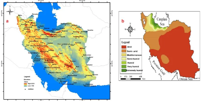
Iran, located between 25° - 40° N and 45°- 60°E, has diverse climate regimes due to wide latitude, Alborze and Zagros mountain chains in north and west, vast deserts (the Kavir and Lut Deserts). North of Iran is limited by Caspian Sea and south of Iran is constrained by Persian Gulf and Oman Sea. According to (De Martonne, 1926, the main climate zones include: arid, semi-arid, Mediterranean, Semi-arid, humid, very humid, and extremely humid.
Fig. 1. a) Topographic map and weather stations of the study area. b) the climate classification of Iran based on De Martonne climate type (1966- 2005) (Tabari et al., 2014)
2.2. Data and Methodology
Data including Air temperature, relative humidity, and pressure in three hourly intervals were obtained from 105 synoptic stations of
series and missed data were excluded from dataset. The applied air DTC model in this
study is based on (Gholamnia et al., 2017):
Ta−day(t) = Tmin+ (Tmax− Tmin) cos ( π
ωair(t − tm)) (1)
Ta−nigth(t) = Tmin+ [(Tmax− Tmin) cos ( π
ωair(ts− tm))] e
(t−ts)
k t > ts (2)
ωair= ω + 2 β (3)
k =ωair
π tan −1( π
ωair(ts− tm)) (4)
Where, Ta is the air temperature (˚C) at time
t; Tmin and Tmax are two variables of minimum
and maximum diurnal air temperatures; tm is
the time when maximum diurnal air temperature occur, ts is the turning point of DTC model, ω
is day duration, and ωair is modified day
duration indicating the width over the half period of the cosine term. β is a coefficient which was used to tune the period of cosine term with air temperature changes. In order to calculate β, the values of 105 synoptic stations the proposed methodology in (Gholamnia et al., 2017) was applied and the range of β was defined between 0 and 10.
Day duration was calculated by (Duffie and Beckman, 1980):
ω = 2
15 arccos(−tanφ tanδ) (5)
φ is latitude and δ is solar declination dependent on day of year (DOY) based on ELAGIB∗et al. (1999):
δ = 23.45 sin (360
365(284 + DOY)) (6)
The behavior and sensitivity of β to environmental variables of humidity, diurnal temperature range, pressure and wind speed were analyzed; in the first step the spatial behavior of β values for 12 months were shown over study area by using Kriging interpolation method. After that variation bars (mean values with standard deviation) were applied to show the behavior of β in contrast with each environmental variable in each month. Finally,
the monthly average of environmental variables was plotted with β values to analyze the general trends in one year period for all weather stations in the study area and their effects on β were discussed.
3. Results
3.1. Estimation of β in the study area
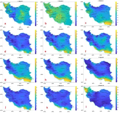
The estimated βvalues were shown in figure (2) for each month in the study area. In January the maximum β was 2.6 in North West of Iran (Figure 2a). In February (Figure 2b), β was decreased in North West but in other areas it had slight increase. In March (Figure 2 C), β had slight decrease except for south east of the study area. In April (Figure 2d), β increased significantly specially at south part of Iran with 9.2. The spatial extent of high β values in south, south west, south east and central part of Iran was increased and reached maximum in May, June and July (Figure 2 e, f, and g). In July the values of β were decreased up to December (Figure 2 h, i, j, k, and l).
3.2. The accuracy of air temperature modeling
Fig. 2. The spatio-temporal behavior of β in the study area; a) January, b) February) March, d) April, e) May, f) June, g) July, h) August, i) September, j) October, k) November, and l) December
3.3. Annual analysis of environmental variables and their relation to β
The humidity pattern in the study area was shown in Figure (4) for each month. In January (figure 4 a) in west, south west, north and north east of Iran, the relative humidity is more than 60 %. In south part (near coast stations) the humidity was almost 55%. The central part, east and south east had relative humidity less than 55%. In February, March, April, May, June, July, August, September, and October (Figure 4 b, c, d, e, f, g, h, i, and j) the humidity in north of Iran was more than other parts (more than 60%). The humidity in May was increased slightly in northwest and west of Iran which can be attributed to the activity of convective
systems during this month of the year (Alijani and Harman, 1985). In south part in near coast stations, the relative humidity was higher in warm periods of year due to the effect of high irradiation and sea breeze. In November and December, the relative humidity was increased in Northwest, west, and north east again. The annual trend showed that in central and eastern parts of Iran, the relative humidity was decreased in warm period of year. The temporal variations in north of Iran had the lowest variation of humidity (minimum humidity range was 4% in Jirandeh in north of Iran). In most of weather stations the humidity was decreased in warm seasons. West of the study area showed high humidity variations (maximum variation was 56.67% in Qasreshirin).
Fig. 4. The spatio-temporal behavior of humidity through a year in the study area; a) January, b) February) March, d) April, e) May, f) June, g) July, h) August, i) September, j) October, k) November, and l) December
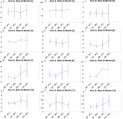
Figure (5) shows the variation bars of mean humidity and its standard deviation against β values for every month (from January to
between 1.9 and 2.3 (Figure 5 a). In February and March, mean β values had slight decrease below 2 (Figure 5 b and c). The pattern of mean β variations in these three months are almost the same; in class three of humidity a slight decrease is observed. After that, the mean β range was increased and in April, except for class two of humidity, mean β had an almost increasing trend (Figure 5d). In May (Figure 5 e), β had a decreasing trend up to class three of humidity and then increased. In June the range of β range was increased and the maximum value (5.8) was observed at fourth level of humidity (Figure 5 f). In July (Figure 5 g), the β range still grew and except for group two it has an increasing trend. In August (Figure 5 h), the
same trend as July was almost observed and the β range was decreased slightly. In September (Figure 5 i) the β reached its maximum value (6.3) in the third group of humidity. In October (Figure 5 j), the range of β decreased suddenly in group three of humidity and has the maximum value of 3.4. In November (Figure 5 k) the curve of plot is reverse in contrast with other plots and has the maximum value in the second class of humidity. In December (Figure 5 l) the trend of plot has an increasing trend from first to forth class of humidity. The general analysis of all variation bars showed no specific trend for humidity and mean β. It is clear that mean β had an increasing trend after March and then decreased after October.
Fig. 5. Variation bars of mean and standard deviation of relative humidity against different β classes; a) January, b) February) March, d) April, e) May, f) June, g) July, h) August, i) September, j) October, k) November, and l) December
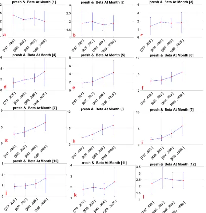
In figure (6) the monthly patterns of pressure in the study area were shown. The results (Figure 6 a, b, c, d, e, f, g, h, I, j, k, and l)
coast) which has low elevation almost 20 m AMSL had highest pressures in the study area (more than 960 hPa). In mountainous regions, west and north west, the pressure was lower in
contrast with other parts. One should note that since no weather station is present in Alborz Mountains in north of Iran, the pressure values at this part were not interpolated properly.
Fig. 6. The spatio-temporal behavior of pressure in the study area; a) January, b) February) March, d) April, e) May, f) June, g) July, h) August, i) September, j) October, k) November, and l) December
The variation bars of mean β and mean pressure for each month is shown in figure (7). Based on annual maximum observed pressure range in weather stations, four classes were defined. In January, February, and March (Figure 7 a, b and c), almost the same pattern
Fig. 7. Variation bars of mean and standard deviation of relative pressure against different β classes; a) January, b) February) March, d) April, e) May, f) June, g) July, h) August, i) September, j) October, k) November, and l) December
The mean of temperature range at each month were shown in Figure (8) in the study area. The spatial pattern of temperatures at each month did not show a specific behavior. This showed that spatial behavior of mean temperature range in the study area is complex
Fig. 8. The spatio-temporal behavior of temperature range in the study area; a) January, b) February) March, d) April, e) May, f) June, g) July, h) August, i) September, j) October, k) November, and l) December.
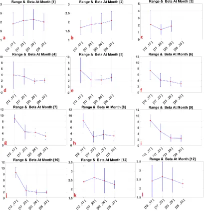
In Figure (9) the variation bars of mean diurnal temperature range and β values at each month are shown. The diurnal temperature range was divided to four classes based on maximum observed mean diurnal temperature range in weather stations. In January, February, and March β did not changed significantly in four classes (Figure 9 a, b, c). From April to November (Figure 9 e, f, g, h, I, j, and k), β experienced significant ranges almost between 2 and 8.9 (in July it had the maximum value). The
Fig. 9. Variation bars of mean and standard deviation of mean diurnal air temperature against different β classes; a) January, b) February) March, d) April, e) May, f) June, g) July, h) August, i) September, j) October, k) November, and l) December
In figure (10) the mean of wind speed were shown at each month in the study area. In January, February and March (figure 10 a, b and c) the pattern of wind speed is almost the same and central part of study area had higher values and the wind speed increased (between 3.2 and 3.8). In April, May, June, and July (Figure 10 d, e, f, and g) the mean wind speed was increased specially in eastern and south eastern parts
Fig. 10. The spatio-temporal behavior of wind in the study area; a) January, b) February) March, d) April, e) May, f) June, g) July, h) August, i) September, j) October, k) November, and l) December
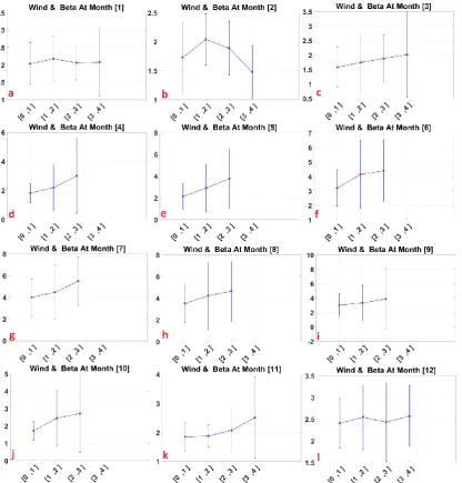
Figure (11) shows the variations of mean wind speed in contrast with β for each month. The wind speed was classified based on the maximum observed range. From April to August the range of β increased and reached its maximum in July (5.7) (Figure 11 c, d, e, f, and
Fig. 11. Variation bars of mean and standard deviation of wind against different β classes; a) January, b) February) March, d) April, e) May, f) June, g) July, h) August, i) September, j) October, k) November, and l) December
In order to analyze the annual variations of β, the mean values of all environmental variables were calculated for one year and the variation bars were shown (Figure 12). In figure (12 a), the variation bar of β values against humidity classes were shown. In class two of humidity (30 to 50) an abrupt decrease in β is observed and an increasing trend is happened but the total range of β did not change significantly. The maximum variation in β values was observed at fourth class of humidity. Based on the results from figure (5) it can be concluded that the humidity can have a direct effect on β. Figure (12 b) shows the variation of β against with pressure classification. As the variation bar shows as far as pressure increases, the β increased. Also, the variations of β at each
the study area has high β value and lower diurnal temperature range. In Figure (3 c) the β is the largest in comparison to last stations. The diurnal temperature range in Jask station was the lowest (less than 2 °C) and the RMSE of fitting is the largest (1.37 °C). Figure (12 d)
shows the β values against mean wind speeds. By mean wind speed increase, the β values increased. Also, the variations of β around mean were increased from the first to the third class but in the fourth class it decreased significantly.
Fig. 12. The variation bars of mean and standard deviation of relative mean diurnal air temperature against different β classes in one year; a) humidity, b) pressure) mean diurnal temperature range, d) wind
Fig. 13. The DTC model and air temperature observations in three sample weather stations; a) Abali, b) Boushehr, and c) Jask
5. Discussion and Conclusion
The diurnal modeling of air temperature by DTC model was implemented over Iran with RMSE of less than 2.1° C in 95% percent of data and the sensitivity of β coefficient as a dynamic variable in relation to environmental variables of humidity, pressure, diurnal temperature range, and wind speed were analyzed. The results showed that the accuracy of air DTC modeling did not have significant difference by considering β both as constant (for one year) or dynamic parameter (monthly) through the year. The variability of β showed significant monthly differences at each weather station and weather stations in south of Iran had the maximum values at most of months (Konarak station had maximum variation between 0.9 and 10 ). The relationships between β and environmental factors of humidity,
spatial pattern but the humid regions in north and south of the study area had lowest variations. Diurnal temperature range show negative relation with β; as far as the diurnal temperature increases the standard deviation and values of β decreased; by increase of temperature range the β values experience lower standard deviations (between 1.8 and 2.5). This may shows that in desert areas with high diurnal temperature ranges, the β values were the lowest and in high lands they were highest. Wind variable showed positive effect on β; the more the wind speed increased, the more mean of β values were increased. This can be concluded that in areas with higher wind values, the β values should increase to fit the mathematical model DTC to temperature observations. The results from this study can be applicable in many disciplines. It is necessary to conduct researches in future to analyze future the effect of environmental variables at each climate regime on β values. Also, it would be beneficial if the performance of different DTC approaches be compared to the study area.
Acknowledgments
The authors deeply thank the Iranian National Science Foundation and Iranian National Space Administration for their great support in conducting this research.
References
Aikawa, M., T. Hiraki, J. Eiho, H. Miyazaki, 2008. Role of the wind in the control of the air temperature distribution. Meteorology and Atmospheric Physics, 102; 15-22.
Alijani, B., J. R. Harman, 1985. Synoptic climatology of precipitation in Iran. Annals of the Association of American Geographers, 75; 404-416.
Benali, A., A. Carvalho, J. Nunes, N. Carvalhais, A. Santos, 2012. Estimating air surface temperature in Portugal using MODIS LST data. Remote Sensing of Environment, 124; 108-121.
Bonnardot, V., V. Carey, S. Cautenet, 2017. Diurnal wind, relative humidity and temperature variation in the Stellenbosch-Groot Drakenstein wine-growing area. South African Journal of Enology and Viticulture, 23; 62-71.
De Kauwe, M. G., B. E. Medlyn, A. P. Walker, S. Zaehle, S. Asao, B. Guenet, A. B. Harper, T. Hickler, A. K. Jain, Y. Luo, 2017. Challenging terrestrial biosphere models with data from the long term multifactor Prairie Heating and CO2 Enrichment experiment. Global Change Biology, 23; 3623-3645. Duffie, J. A., W. A. Beckman, 1980. Solar engineering of thermal processes. John Wiley & Sons.
Elagib, N. A., S. H. Alvi, M. G. Mansell, 1999. Day- length and extraterrestrial radiation for Sudan: a comparative study. International Journal of Solar Energy, 20; 93-109.
Ephrath, J., J. Goudriaan, A. Marani, 1996. Modelling diurnal patterns of air temperature, radiation wind speed and relative humidity by equations from daily characteristics. Agricultural Systems, 51; 377-393. Gadgil, A., A. Dhorde, 2005. Temperature trends in twentieth century at Pune, India. Atmospheric Environment, 39; 6550-6556.
Geiger, R., R. H. Aron, P. Todhunter, 2009. The climate near the ground. Rowman & Littlefield.
Gholamnia, M., S. K. Alavipanah, A. Darvishi Boloorani, S. Hamzeh, M. Kiavarz, 2017. Diurnal Air Temperature Modeling Based on the Land Surface Temperature. Remote Sensing, 9; 915.
Haas, E., S. Klatt, A. Fröhlich, P. Kraft, C. Werner, R. Kiese, R. Grote, L. Breuer, K. Butterbach-Bahl, 2013. LandscapeDNDC: a process model for simulation of biosphere–atmosphere–hydrosphere exchange processes at site and regional scale. Landscape Ecology, 28; 615-636.
Hansen, J., S. Lebedeff, 1987. Global trends of measured surface air temperature. Journal of geophysical research: Atmospheres, 92; 13345-13372.
Jones, P. D., M. New, D. E. Parker, S. Martin, I. G. Rigor, 1999. Surface air temperature and its changes over the past 150 years. Reviews of Geophysics, 37; 173-199.
Leuning, R., F. Kelliher, D. d. Pury, E. D. Schulze, 1995. Leaf nitrogen, photosynthesis, conductance and transpiration: scaling from leaves to canopies. Plant, Cell & Environment, 18; 1183-1200.
Lofgren, B. M., 2014. Simulation of atmospheric and lake conditions in the Laurentian Great Lakes region using the Coupled Hydrosphere-Atmosphere Research Model (CHARM). NOAA Tech. Memo. GLERL-165, 23 pp.[Available online at http://www. glerl. noaa. gov/ftp/publications/tech_reports/glerl- 165/tm-165. pdf.].
Lowen, A. C., S. Mubareka, J. Steel, P. Palese, 2007. Influenza virus transmission is dependent on relative humidity and temperature. PLoS Pathog, 3; e151. Nojarov, P., 2014. Atmospheric circulation as a factor for air temperatures in Bulgaria. Meteorology and Atmospheric Physics, 125; 145-158.
Parton, W. J., J. A. Logan, 1981. A model for diurnal variation in soil and air temperature. Agricultural Meteorology, 23; 205-216.
Peng, S., J. Huang, J. E. Sheehy, R. C. Laza, R. M. Visperas, X. Zhong, G. S. Centeno, G. S. Khush, K. G. Cassman, 2004. Rice yields decline with higher night temperature from global warming. Proceedings of the National academy of Sciences of the United States of America, 101; 9971-9975.
Péré, J., B. Bessagnet, M. Mallet, F. Waquet, I. Chiapello, F. Minvielle, V. Pont, L. Menut, 2014. Direct radiative effect of the Russian wildfires and its impact on air temperature and atmospheric dynamics during August 2010. Atmospheric Chemistry and Physics, 14; 1999-2013.
Philandras, C., P. Nastos, I. Kapsomenakis, C. Repapis, 2015. Climatology of upper air temperature in the Eastern Mediterranean region. Atmospheric Research, 152; 29-42.
Prihodko, L., S. N. Goward, 1997. Estimation of air temperature from remotely sensed surface observations. Remote Sensing of Environment, 60; 335-346.
temperature, atmospheric precipitable water and vapor pressure deficit using Advanced Very High- Resolution Radiometer satellite observations: comparison with field observations. Journal of Hydrology, 212; 230-249.
Qu, M., J. Wan, X. Hao, 2014. Analysis of diurnal air temperature range change in the continental United States. Weather and Climate Extremes, 4; 86-95. Stensrud, D. J., 2009. Parameterization schemes: keys to understanding numerical weather prediction models. Cambridge University Press.
Stisen, S., I. Sandholt, A. Nørgaard, R. Fensholt, L. Eklundh, 2007. Estimation of diurnal air temperature using MSG SEVIRI data in West Africa. Remote Sensing of Environment, 110; 262-274.
Sun, D., R. T. Pinker, M. Kafatos, 2006. Diurnal temperature range over the United States: A satellite view. Geophysical Research Letters, 33.5
Tabari, H., P. H. Talaee, 2011. Recent trends of mean maximum and minimum air temperatures in the western half of Iran. Meteorology and Atmospheric Physics, 111; 121-131.
Tabari, H., P. H. Talaee, S. M. Nadoushani, P. Willems, A. Marchetto, 2014. A survey of temperature and precipitation based aridity indices in Iran. Quaternary International, 345; 158-166.
Tanja, S., F. Berninger, T. Vesala, T. Markkanen, P.
Hari, A. Mäkelä, H. Ilvesniemi, H. Hänninen, E. Nikinmaa, T. Huttula, 2003. Air temperature triggers the recovery of evergreen boreal forest photosynthesis in spring. Global Change Biology, 9; 1410-1426.
Türkeş, M., U. Sümer, 2004. Spatial and temporal patterns of trends and variability in diurnal temperature ranges of Turkey. Theoretical and Applied Climatology, 77; 195-227.
Walthall, C., J. Hatfield, E. Marshall, L. Lengnick, P. Backlund, S. Adkins, E. Ainsworth, F. Booker, D. Blumenthal, J. Bunce, 2013. Climate Change and Agriculture: Effects and Adaptation.
Xia, G., L. Zhou, J. M. Freedman, S. B. Roy, R. A. Harris, M. C. Cervarich, 2016. A case study of effects of atmospheric boundary layer turbulence, wind speed, and stability on wind farm induced temperature changes using observations from a field campaign. Climate Dynamics, 46; 2179-2196. Yue, S., M. Hashino, 2003. Temperature trends in Japan: 1900-1996. Theoretical and Applied Climatology, 75; 15-27.