0 BACKGROUND
Pump failures induce rapid changes in the flow rate, which causes extremely high-pressure water hammer surges in the water supply system, including extremely high- and low-pressure water hammer surges. Extreme water hammer pressure damages pipes and hydraulic equipment and results in water supply service interruptions. To eliminate or reduce the impact of extreme water hammer pressure on water delivery systems, water hammer prevention measures are normally implemented; these include bypass pipes, air valves, check valves, air tanks, pressure regulating chambers, unidirectional pressure regulating chambers, pressure discharge valves, water hammer prevention valves, etc. [1] to [3]. An air valve is a common, economical, and effective piece of water hammer prevention equipment that is normally installed at the local peak of a pipe. When negative pressure occurs inside the pipe, the air valve opens to allow air in; when the pressure inside the pipe increases, the air valve releases it by discharging air [4] and [5]. A check valve is an economical and
reasonable water hammer prevention measure that is widely used in pumping stations [6]. Check valves can prevent water pumps from rotating in reverse due to liquid backflow and thus prevent damage to the motor. However, instant check valve closure results in a catastrophically high pressure [7] and [8]. Therefore, when a check valve is installed in a pumping station to control transients, an air tank should also be installed near the pumping station to prevent the increase in pressure that results from closing the check valve [9]. However, air tanks have drawbacks that include their large volume, high maintenance cost and complex operation (the gas in the tank should be replenished). A pressure discharge valve with the proper parameters can prevent a water delivery system from generating excessively high or low pressures; otherwise, the negative impact of water hammer surges on the water delivery system is exacerbated [10]. To ensure proper protection of a water delivery system by a pressure discharge valve, the pressure discharge valve should have so little inertia that it can be opened promptly in response to a rapid change in the pressure to prevent delays in its opening [11]. A water hammer
Numerical Simulation of Transient Pressure Control
in a Pumped Water Supply System
Using an Improved Bypass Pipe
Li, X.– Zhu, M.– Xie, J.
Xiaozhou Li– Manlin Zhu* – Jiancang Xie
Xi’an University of Technology, State Key Laboratory Base of Eco-hydraulic Engineering in Arid Area, China
The use of a bypass pipe in a pump system is an economical and simple method of preventing water hammer surges to control the extreme transient pressures induced by pump failure. Currently, conventional bypass pipes (CBPs) have certain limitations in engineering applications. To overcome these limitations, in this study, a CBP is modified to create an improved bypass pipe (IBP). Unlike that of a CBP, the control valve in an IBP system is a hydraulic control valve that uses a controller on an uninterruptible power source (UPS) to turn the valve on or off. This modification enables the hydraulic control valve to be precisely controlled and facilitates the prevention of water hammer surges. To study the transient control effect of the IBP using the method of characteristics (MOC), a mathematical model of a complex system that includes an IBP, a check valve, and a water pump is established. Using MATLAB software, a water supply system in an industrial zone is used as an example for numerical simulations of the transient process experienced by this pump after it fails. The extreme pressure variations and the envelope of the pipe pressure in a typical section of the pumped water supply system are analysed and compared. The results show that an IBP can effectively reduce the maximum extreme pressure in a pumped water supply system.
Keywords: improved bypass pipe, hydraulic transient, pumped water supply system, UPS controller, numerical simulation Highlights
• Based on a conventional bypass pipe, a new, economical, and effective water hammer prevention measure, i.e., an improved bypass pipe, is proposed.
• A hydraulic control valve with an on/off status determined by an uninterruptible power source controller is installed in the bypass pipe to control the transient pressure.
• The on/off time for the newly developed improved bypass pipe is accurately controlled to facilitate transient pressure control. • Based on the method of characteristics, a mathematical model for a complex system containing an improved bypass pipe is
prevention valve may have inaccurate hydraulic control that causes its opening to be delayed, or that causes it to close excessively fast, which results in water hammer damage. Wylie [12] proposed two types of conventional bypass pipes (CBPs) for preventing water hammer surges in pumping stations. One was to install a check valve in the water pump’s outlet and a control valve in the bypass pipe to prevent the pump from rotating in reverse due to water backflow. After pump failure, the bypass pipe control valve opens instantly and then closes gradually to release the high pressure inside the system and eliminate water hammer surges. The other type was designed to prevent low pressure and water column separation in the water pump’s outlet from being caused by pump failure. A control valve was installed at the water pump’s outlet, and a check valve was installed in the bypass pipe; therefore, the water flowing into the reservoir could be directed to the water pump’s outlet through the bypass pipe. Both types of CBPs have certain drawbacks. The first type of bypass pipe cannot accurately control the valve’s on/off timing; therefore, it may not be able to prevent water hammer surges as well as is desired. The second type of bypass pipe cannot release the high pressure in the system and is only applicable to pumping station water supply systems that ignore the effect of backflow and have water pump inlets with positive water head pressures.
Compared with experimental studies, numerical simulations take less time and are more economical. With advances in computer technology, numerical simulations have become widely employed in water hammer analyses [13] to [15]. To predict pressure variations in a water supply system and to choose appropriate water hammer preventive measures, numerical simulations of water hammer surges are indispensable, simple, and effective [16]. Methods of numerically analysing water hammer surges include arithmetic, graphical, algebraic and linear analysis methods as well as the method of characteristics (MOC). At present, the MOC is the simplest and most popular method for numerically solving transient flow problems. Izquierdo proposed mathematical models for simulating transient boundary conditions in simple and complex hydraulic systems [17] and [18]. Because the results of hydraulic transient numerical simulations are in good agreement with those of test measurements [19] and [20], the results of numerical simulations of water hammer surges are widely accepted.
A composite bypass pipe and check valve is installed in a pumping station to reduce the extremely high water pressure associated with water hammer
surges in a pumped water supply system. However, this type of CBP has limitations. Therefore, this study has three purposes:
1) To overcome the limitations of CBPs, an improved bypass pipe (IBP)-based water hammer prevention measure is proposed, and the operational principle of an IBP is explained. 2) Based on previous studies and the method of
characteristics (MOC), a mathematical model of the boundary conditions of an IBP is established, and a solution for this mathematical model is described.
3) A water supply system in an industrial zone is used as an example in a numerical simulation of the water hammer prevention effect of a pump with an IBP-based protective device on a water supply system and to provide evidence for the use of an IBP-based water hammer prevention measure in a system.
1 THE STRUCTURE AND OPERATIONAL PRINCIPLE OF THE IMPROVED BYPASS PIPE
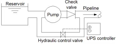
Fig. 1 shows a diagram of the IBP. It is based on a CBP, but the control valve in the CBP is replaced by a hydraulic control valve. The hydraulic control valve consists of a valve body, a hydraulic pressure system, an oil cylinder, an energy storage tank, and an electromagnetic valve. The IBP’s hydraulic control valve leverages an uninterruptible power source (UPS), which provides power to the electromagnetic valve, which controls when and for how long the main valve is open. This improvement can prevent the valve from turning on or off in response to man-made or hydraulic interference and provide more accurate control over the valve’s status than a conventional manually or hydraulically controlled valve can.
Fig. 1. Schematic of the IBP
After the pump fails, the UPS-powered controller can predefine a delayed opening time,
rod-less chamber of the oil cylinder and rotates the valve board to open the main valve. The main valve’s opening time, t2 (the time it takes the main valve to
make the transition from being completely closed to being completely open), is regulated via the pressure at the valve that controls the oil’s flow rate according to actual requirements. After the time allotted for the electromagnetic valve to be open expires, the UPS-powered controller closes the electromagnetic valve, and the oil in the energy storage tank enters the rod chamber of the oil cylinder and pushes the piston back to close the main valve. The main valve’s closing time, t4 (the time it takes for the main valve to make
the transition from completely open to completely closed), is regulated by a valve closure regulation valve according to actual requirements. The difference between the time for which the electromagnetic valve is open and the time required for the main valve to open is defined as the main valve’s opening duration,
t3 (the time the main valve is completely open). Fig. 2
shows the IBP in operation.
Fig. 2. Flowchart of the IBP’s operation
2 CHARACTERISTIC EQUATIONS FOR CALCULATING WATER HAMMER SURGES AND THEIR SOLUTION
2.1 Basic Differential Equations for Water Hammer Surges
The basic differential equations for water hammer surges consist of an equation of motion Eq. (1), and a continuity equation, Eq. (2).
∂ ∂ +
∂ ∂ +
∂
∂ + =
h x g
v t
v g
v x
f D
v v g 1
2 0, (1)
∂
∂ +
∂
∂ − +
∂
∂ =
h t v hx
a g
v x
( sin )θ .
2
0 (2)
2.2 Simplified Finite-Difference Equations
The numerical calculation of water hammer surges is based on comprehensive and complete basic differential equations, Eqs. (1) and (2). These two
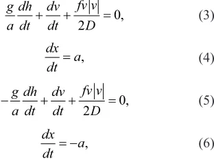
equations comprise a pair of non-linear hyperbolic partial differential equations, which is very difficult to solve using conventional methods. Therefore, the MOC is used to convert the two partial differential equations that take pipeline hydraulic friction into account into ordinary differential equations of a specific form. These are called characteristic equations and are given in Eqs. (3) and (4) for C+ andin Eqs. (5)
and (6) for C–:
g a
dh dt
dv dt
fv v D
+ + =
2 0, (3)
dx
dt =a, (4)
−g + + =
a dh dt
dv dt
fv v D
2 0, (5)
dx
dt = −a, (6)
where, because ν sinθ is typically much smaller compared with any other item in the equation for the transient process and because wave speed a is far larger than the flow velocity ν, ν sinθ is ignored in Eq. (3) and Eq. (5), and the flow velocity, ν, is ignored in Eq. (4) and Eq. (6).
Next, the characteristic equations are integrated to generate a set of simplified finite-difference equations, Eqs. (7) to (10).
C h+ i j t=Cp−BQi j t
: ,∆ ,∆, (7)
C h− i j t=CM +BQi j t
: ,∆ ,∆, (8)
CP =hi−1,(j−1)∆t+BQi−1,(j−1)∆t−RQi−1,(j−1)∆t Qi−1,(j−1)∆t , (9)
CM =hi+1,(j−1)∆t−BQi+1,(j−1)∆t−RQi+1,(j−1)∆t Qi+1,(j−1)∆t . (10)
In Eqs. (7) to (10) B = a/(gA), R = fΔx/(2gDA2), hi–1,( j–1)Δt, hi+1,( j–1)Δt, Qi–1,( j–1)Δt and Qi+1,( j–1)Δt, and
are known from the previous step; only hi,jΔt and Qi,jΔt
are unknown.
2.3 Procedure for Solving the Water Hammer Equations
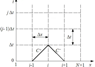
Fig. 3 shows the grid diagram used in the MOC. The solution process normally starts with a stable flow at
t = 0. Therefore, the initial values of h and Q in each calculation section are known. Based on their values at t = 0 in all the sections of a layer, the values of h and
of the layer are calculated. The same procedure is followed until values at the required time, t = jΔt, are calculated.
Fig. 3. A characteristic line in space (x) - time (t)
3 BOUNDARY CONDITIONS AND A MATHEMATICAL MODEL FOR THE IBP
Fig. 4 shows that the check valve and the controllable bypass pipe composite are installed at the pump’s outlet to prevent water hammer surges. The check valve is installed at the water pump’s outlet to prevent backflow in the water delivery pipe due to accidental power failure and to facilitate maintenance and repairs. However, a check valve by itself may close suddenly and cause damage if there is a water hammer surge resulting from a pump failure or if there is a severe engineering accident. Therefore, installing a controllable bypass pipe can prevent an increase in pressure resulting from a sudden closure of the check valve. To study the water hammer prevention effect of a controllable bypass pipe, the MOC is employed to perform a numerical analysis and calculations. The MOC is a widely used numerical method that is verified in reference [12].
Before establishing a mathematical model, the following assumptions are made:
1. From when the pump fails to when the flow rate at the water pump’s outlet drops to zero, the check valve local coefficient of resistant is a constant,
kc1, and when the flow rate at the water pump’s outlet is Q6 ≤ 0, the check valve closes instantly.
2. The local water head losses at T-type nodes upstream and downstream of the water pump are ignored.
3. The T-type nodes connecting the pipe and the bypass pipe upstream and downstream of the water pump (the dashed box in Fig. 4) are very short, and loss during the flow is ignored; they are analysed as an integral unit.
When a power failure occurs, the water pump in the water supply system suddenly loses power, the pump’s outlet pressure drops, and water flows back. When the flow rate at the water pump’s outlet is less than or equal to zero (Q6,( j–1)Δt = 0), the check valve
closes instantly (Q6, jΔt = 0). When the pump fails at
time T ≤ t1, the IBP closes (Q4, jΔt = Q5, jΔt = 0). When the
pump fails at time t1 < T < t1+t2+t3+t4 , the IBP opens
quickly and stays open. At this point, the backflow water column is discharged from the IBP to the reservoir. When the pump fails at time T ≥ t1+t2+t3+t4 ,
the IBP closes slowly (Q4, jΔt = Q5, jΔt = 0).
Fig. 4. A boundary model of the IBP Continuity equation:
Q Q Q Q Q Q
Q Q Q
j t j t j t j t j t j t
j t j t
2 3 4 7 5 6
3 6
, , , , , ,
, ,
, ,
∆ ∆ ∆ ∆ ∆ ∆
∆ ∆
= + = +
= =υ RR, Q4,j t∆ =Q5,j t∆, (11)
water balance equation:
h H a b
kc Q Q
gA
j t R
j t j t
3
2 2 0
1 0
1
3 3
2 ,
, ,
( tan )
∆
∆ ∆
+
(
+)
+ +
−
−
−
α υ π υ
α
1 1
2 6
4 2
4 4
2
2 5
2 3
2 =
− =
=
h
h kc Q Q
gA h
h h
j t
j t j t j t j t
j t j t
,
,
, , ,
, ,
, ∆
∆
∆ ∆
∆
∆ ∆==h4,j t∆, h5,j t∆ =h6,j t∆=h7,j t∆, (12)
characteristic equation:
h2,j t∆ =CP−B Q1 2− 2,j t∆, h7,j t∆ =CM +B Q7 8− 7,j t∆, (13) water pump’s unit inertia equation:
α υ π υ
α β
π α α
2 2 1
1
1 0
2
0
15 0
+
(
)
+ +
+ −
− − =
−
a b
WR g
N TRR t
( tan )
( ) .
∆ (14)
F C C B B Q Q
H a b
P M R j t
R
1 1 2 7 8 4
2 2 0 1 = − −
(
+)
(
+)
+ +(
+)
+ + − − − υ α υ π υ α ,( tan )
∆ 0 0 1 1 2 2 0 −
−kc Q =
gA
Rυ υ , (15)
F C C B B Q Q
kc Q Q
gA
P M R j t
j t j t
2
2 0
1 2 7 8 4
2 4 4 2 2 = − −
(
+)
(
+)
− − = − − υ , , , , ∆ ∆ ∆ (16)F a b
WR g
N TRR t 3 15 0 2 2 1 1 1 0 2 0 =
(
+)
+ + + + − − = − α υ π υ α β π α α( tan )
( )
∆ .. (17)
Eq. (15), Eq. (16) and (17) can be solved using the Newton-Raphson method [12].
F F B B Q
H a b a
R
R
1 1
2
1 2 7 8
0 1 0 υ υ υ π υ α =∂ ∂ = − + + + + + + − − − ( )
tan 00 1
1 2 α υ
−kc QgA
R , (18)
F1 F HR a b a
1
2 0 1
0 0 α α α π υ α υ =∂ ∂ = + + − −
tan , (19)
F F
Q B B
Q j t j t 1 1 4 4
1 2 7 8 , , ( ), ∆ ∆ = ∂
∂ = − − + − (20)
F2υ = Fυ2 B1 2 B Q7 8 R ∂
∂ = −( − + − ) , (21)
F2α F2 0
α =∂
∂ = , (22)
F F
Q B B kc
Q gA Q j t j t j t 2 2 4 4
1 2 7 8 2 4 2 2 , , , ( ) , ∆ ∆ ∆ = ∂
∂ = − − + − − (23)
F3 F3 2 a1 b a
1 1 1 υ υ υ π υ α α =∂ ∂ = + + + −
tan , (24)
F F a b
a WR
g N TRR t
3 3 2
15 1 1 1 1 2 α α α π υ α υ π =∂ ∂ = + + − − + − tan ,
∆ (25)
F F
Q
Q
j t
j t
3 3 0
4 4 , , . ∆ ∆ = ∂
∂ = (26)
The Newton-Raphson equations are represented as matrices:
F F F
F F F
F F F
Q Q Q j t j t j t
1 1 1
2 2 2
3 3 3
4 4 4 υ α υ α υ α υ α , , , ∆ ∆ ∆ ∆ ∆ ∆∆Q ∆
F F F j t 4 1 2 3 , . = − − − (27)
Initial values are assigned to υ and α as follows:
υ= υ −υ α= α −α = − − − − − 2 2 2
1 2 1 2
4 4 1
( ) ( ) ( ) ( )
, ,( )
, ,
j t j t j t j t
j t j
Q Q
∆ ∆ ∆ ∆
∆ ∆∆t−Q4,(j−2)∆t. (29)
Eqs. (15) to (26) are substituted into Eq. (28) and solved for Δυ, Δα and ΔQ4, jΔt . Then, Eq. (29) is
rewritten as:
υ υ= +∆υ α α, = +∆α, Q4,j t∆ =Q4,j t∆ +∆Q4,j t∆. (30)
The above procedure is repeated until Δυ, Δα
and ΔQ4, jΔt are within the allowable deviation range:
|Δυ|+|Δα|+|ΔQ4, jΔt| < ε.
The allowable deviation ε is set to approximately 0.0002 [12].
The solutions of the above equations are represented as matrices,
∆ ∆ ∆ ∆ ∆ ∆ υ α υ α α υ
Q F F F F F F
F
j t Q Q
Q
j t j t 4
1
1 2 3 1 2 3
1 4 4 4 , ( , , = + + ,, , , , )
j t j t
j t j t
F F F F F
F F F F F F
F
Q
Q Q
∆ ∆
∆ ∆
2 3 1 2 3
1 2 3 1 2 3
4 4 4 υ α α υ υ α α υ − − − 2
2 3 2 3 1 3 1 3 1 2
4 4 4 4 4
αF Q,j t∆ −F Q,j t∆F α F Q,j t∆ F α −F Fα Q,j t∆ F Fα Q,j t∆ −FF F
F F F F F F F F
Q
Q Q Q Q
j t
j t j t j t j t
1 2
2 3 2 3 1 3 1 3
4
4 4 4 4
,
, , , ,
∆
∆ ∆ ∆ ∆
α
υ− υ υ − υ FF F F F
F F F F F F F F F F F
Q j t Q j t
1 2 1 2
2 3 2 3 1 3 1 3 1 2
4,∆ υ υ 4,∆
υ α α υ α υ υ α υ α
−
− − − 11 2
1
2
3 αF υ
F F F − − −
4 USE OF AN IBP IN A PUMPED WATER SUPPLY SYSTEM
4.1 System Overview
As shown in Fig. 5, a pumping station water supply system consists of three identical water pumps operating in parallel, two parallel pipes, and upstream and downstream reservoirs. The pumping station’s static head is 142 m, the water pump’s rated head is
HR = 149.5 m, the rated flow rate is QR = 0.37 m³/s
and the water pump’s rated rotation speed is
NR = 1450 rpm. The pump’s characteristic curve is
based on data for the specific rotation speed ns = 25
(SI), according to reference [12]. Each pump unit’s extreme moment of inertia is WR2 = 450N·m2. The
pipe length is L = 1390 m, and the pipe’s inner diameter is D = 781 mm. The wave speed is a = 1213 m/s, and the pipe’s coefficient of friction is f = 0.02. When the pump stops and backflow starts, the check valve behind the pump closes immediately, and the bypass pipe control valve opens or closes according to the predefined procedure. According to Appendix B of reference
[12]
, when the check valve is completely open (i.e., the valve’s opening level is τ = 1), its discharge coefficient is Cd = 1.4, and when the checkvalve is completely closed (i.e., the valve’s opening level is τ = 0), its discharge coefficient is Cd = 0. Fig.
6 shows the relationship between the hydraulic control valve’s discharge coefficient and opening level. The relationship between the valve’s discharge
coefficientCd , and its local resistance coefficient, kc,
is shown in Eq. (31).
kc=1Cd
2
. (31)
4.2 Numerical Simulations
Numerical simulations and calculations for two post-pump failure scenarios, without an IBP and with an IBP, are performed for the pumped water supply system shown in Fig. 5.
4.2.1 Case 1: Without an IBP
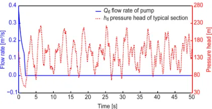
When all three parallel water pumps fail due to an accident and backflow occurs, the check valves behind the pumps immediately close, and the IBP is not involved. The transient process that occurs in the pumped water supply system in this situation is numerically simulated. Fig. 7 shows the flow rate at each water pump’s outlet (Q6) and the typical section
pressure (h6).
Fig. 7. Variations in the flow rate and pressure without an IBP Fig. 7 shows that when the three parallel water pumps fail simultaneously after an accident, the flow rate at each water pump’s outlet (the pipe between the water pump and the main pipe) drops rapidly until
T = 1.99 s, when it becomes negative (i.e., reaches its minimum value), and the typical section pressure at the water head also drops to its minimum value. At this point, the check valve closes instantly to prevent a high volume of backflow, and the flow rate at each water pump’s outlet stabilizes at zero. However, the closure of the check valve also stops the transient high-pressure wave from returning and being discharged, which may lead to an extremely high-pressure water hammer surge in the system.
4.2.2 Case 2: With an IBP
Fig. 8 shows that the hydraulic control valve’s on/ off program opens the IBP 2.5 s after pump failure (t1 = 2.5 s). It takes 3 s (t2 = 3.0 s) to make the transition
Fig. 5. A diagram of a pumped water supply system
from being completely closed to being completely open; it remains completely open for 5 s (t3 = 5 s), and then it takes 15 s (t4 = 15 s) to make the transition from
being completely open to being completely closed.
Fig. 8. Operation of the hydraulic valve
Fig. 9 shows the flow rate at the outlet of a water pump with an IBP and typical variations in the section pressure. Fig. 9 shows that when the three parallel water pumps fail simultaneously, the flow rate at each water pump’s outlet (Q6) also drops rapidly until T = 1.99 s, when it becomes negative (i.e., reaches its minimum value), and the typical section pressure at the water head drops to its minimum value as well. At this point, the check valve closes instantly to prevent a high volume of backflow, and the flow rate at each water pump’s outlet stabilizes at zero. Because the IBP opens at a predefined time, the returned transient high-pressure wave is not blocked by the closed check valve. Instead, it is discharged by the IBP, eliminating the extremely high-pressure water hammer surge from the system. During this period, the maximum flow rate in the IBP reaches Q5 = –1.062 m³/s. In addition, the IBP gradually closes at a predefined time to prevent valve closure-induced water hammer surges.
Fig. 9. The flow rate and pressure variation at the IBP
4.3 Comparison and Analysis of Simulation Results
The mathematical model of the IBP presented in this study is used in numerical simulations and
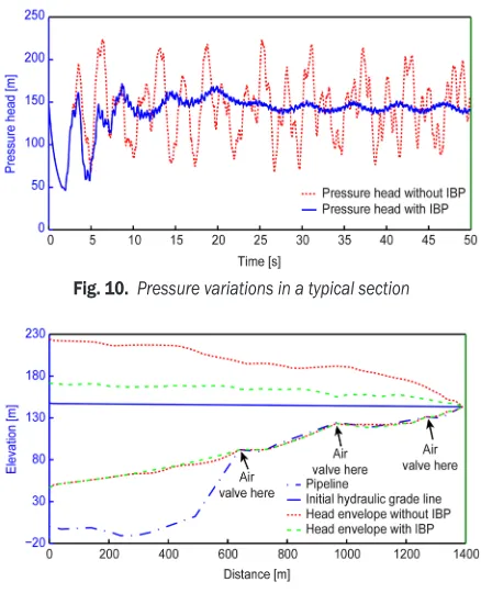
calculations of a transient process in a pumped water supply system. The typical variations in the section pressure determined by the simulations are shown in Fig. 10. In the graph, the red dashed line represents typical variations in the section pressure when there is no IBP, and the solid blue line represents typical variations in the section pressure when there is an IBP. The simulation results show that without an IBP, the water head of the maximum transient pressure in a typical section reaches 223.2 m, which is 1.51 times the initial pressure water head (147.5 m). With an IBP, the water head of the maximum transient pressure in a typical section drops to 171.8 m, which is 1.16 times the initial pressure water head (147.5 m). These results show that the presence of an IBP can significantly reduce the water head of a typical section’s maximum transient pressure.
Fig. 10. Pressure variations in a typical section
Fig. 11. Envelopes of extreme pressure
This graph shows that an IBP significantly reduces the maximum extreme pressure in a pumped water supply system, which ensures that the water supply system operates safely and reliably.
5 CONCLUSIONS AND FUTURE WORK
In a pumped water supply system, pump failure reduces the pressure in the water supply pipe and results in subsequent liquid backflow in the pipe. An enormous backflow not only results in water column separation but also impacts the water pump’s impeller and makes it rotate in reverse. In severe cases, it threatens the pumped water supply system’s safe operation. Check valves are widely used in pumped water supply systems to prevent pump failure-induced water backflow and reverse rotation of the water pump. However, rapid check valve closure also results in extremely high-pressure water hammer surges. Previous researchers combined a CBP with a check valve to release the high pressure in the system and eliminate water hammer surges. However, because the timing of the CBP valve’s on/off setting cannot be accurately controlled, it may not be possible to achieve the desired water hammer prevention effect. To overcome this limitation of CBPs, this study improved the CBP and proposed a new water hammer prevention measure, the IBP. An IBP is a bypass pipe with a hydraulic control valve controller whose on/ off procedure is predefined by a UPS. Therefore, the valve’s setting can be accurately controlled. Using the MOC, a mathematical model of the IBP is established, and calculations are performed. This mathematical model simulates and calculates typical variations in the transient section pressure and the distribution of the pressure in the water supply pipe for a pumped water supply system in an industrial zone. A comparison of the simulation results shows that the IBP (whose hydraulic control valve’s setting is changed at
t1 = 2.5 s, t2 = 3.0 s, t3 = 5 s and t4 = 15 s) water hammer prevention measure in a pumped water supply system can significantly reduce the maximum extreme pressure of water hammer surges in the pumped water supply system. However, some of the problems encountered in this study require further research: 1) The mathematical model of the IBP does not take into account the bypass pipe’s length and diameter; it only considers the bypass pipe valve’s local coefficient of resistance, so the next step is to incorporate the bypass pipe’s length, l, and diameter, d, into the mathematical model to study the effect of the bypass pipe’s length and diameter on water hammer prevention. 2) The numerical simulation and calculation of the pumped
water supply system’s transient process shows that an IBP can protect the water supply system from damage due to water hammer surges; however, the sensitivity of key parameters affecting the IBP’s water hammer prevention effect (the bypass pipe’s length, l, and diameter, d, and the bypass pipe hydraulic control valve’s delayed opening time, t1, opening time, t2, opening duration, t3 and closing time, t4) will analyzed to provide reference parameters for engineering applications.
6 ACKNOWLEDGMENTS
This research program is sponsored by the National Natural Science Foundation of China (Grant Nos. 41471451 and 51479160).
7 NOMENCLATURE
t time [s] T time [s]
h pressure head [m] ν flow velocity [m/s]
g acceleration of gravity [m/s2]
a wave speed of water hammer surge [m/s] x distance along pipe [m]
θ pipe slope
f Darcy-Weisbach friction factor D pipe inner diameter [m] A area of pipe section [m2]
C+ name for forward characteristic line C– name for reverse characteristic line CP known constant in MOC
CM known constant in MOC B known constant in MOC
R known constant in MOC Δx spatial step size [m] Δt time step size [s]
i subscript denoting the position of the section
j number of time segments
N number of pipe segments
A1 area of check valve section [m2] A2 area of hydraulic valve section [m2] kc1 minor loss coefficient of check valve
kc2 minor loss coefficient of hydraulic valve
QR rated discharge of pump [m3/s] HR rated head of pump [m] υ dimensionless pump discharge α dimensionless pump speed ratio
a0, b0 parameters for pump head characteristics
a1, b1 parameters for pump torque characteristics β dimensionless torque ratio
NR rated rotation speed of pump [rpm] TR rated torque of pump [N·m]
π constant F function symbol
ε assigned precision control τ valve opening ratio L pipe length [m]
ns specific speed
Cd discharge coefficient of valve
l bypass pipe length [m] d bypass pipe inner diameter [m]
8 REFERENCES
[1] Boulos, P.F., Karney, B.W., Wood, D.J., Lingireddy, S. (2005). Hydraulic transient guidelines for protecting water distribution systems. Journal American Water Works Association, vol. 97, no. 5, p. 111-124.
[2] Bergant, A., Kruisbrink, A., Arregui, F. (2012). Dynamic behaviour of air valves in a large-scale pipeline apparatus. Strojniški vestnik - Journal of Mechanical Engineering, vol. 58, no. 4, p. 225-237, DOI:10.5545/sv-jme.2011.032.
[3] Ramezani, L. (2015). An exploration of transient protection of pressurized pipelines using air valves, PhD thesis, University of Toronto, Toronto.
[4] Karadžič, U., Bulatović, V., Bergant, A. (2014). Valve-induced
water hammer and column separation in a pipeline apparatus. Strojniški vestnik - Journal of Mechanical Engineering, vol. 60, no. 11, p. 742-754, DOI:10.5545/sv-jme.2014.1882.
[5] Carlos, M., Arregui, F.J., Cabrera, E., Palau, C.V. (2011). Understanding air release through air valves. Journal of Hydraulic Engineering, vol. 137, no. 4, p. 461-469, DOI:10.1061/(ASCE)HY.1943-7900.0000324.
[6] Thorley, A.R.D. (2004). Fluid Transients in Pipeline Systems: A Guide to the Control and Suppression of Fluid Transients in Liquids in Closed Conduits. ASME Press, New York.
[7] Sugiyama, H., Mizobata, K., Ohtani, K., Ohishi, T., Sasaki, Y., Musha, H., Miwa, T. (2003). Dynamic characteristics of a check valve for drain pumps. ASME/JSME 4 Joint Fluids Summer Engineering Conference, p. 2851-2856, DOI:10.1115/ FEDSM2003-45256.
[8] Thorley, A.R.D. (1989). Check valve behavior under transient flow conditions: A state-of-the-art review.
Journal of Fluids Engineering, vol. 111, no. 2, p. 178-183, DOI:10.1115/1.3243620.
[9] Purcell, P. (1997). Case study of check-valve slam in rising main protected by air vessel. Journal of Hydraulic Engineering, vol. 123, no. 12, p. 1166-1168, DOI:10.1061/(ASCE)0733-9429(1997)123:12(1166).
[10] Zhang, K.Q., Karney, B.W., McPherson, D.L. (2008). Pressure-relief valve selection and transient pressure control. Journal American Water Works Association, vol. 100, no. 8, p. 62-69. [11] Chaudhry, M.H. (1987). Applied Hydraulic Transients, 2nd ed.
Van Nostrand Reinhold, New York.
[12] Wylie, E.B., Streeter, V.L., Suo, L. (1993). Fluid Transients in Systems. Prentice Hall, New Jersey.
[13] Kaliatka, A., Vaišnoras, M., Valinčius, M. (2014). Modelling of
valve induced water hammer phenomeno in a district heating system. Computers&Fluids, vol. 94, p. 30-36, DOI:10.1016/j. compfluid.2014.01.035.
[14] Skulovich, O., Perelman, L., Ostfeld, A. (2014). Bi-level optimization of closed surge tanks placement and sizing in water distribution system subjected to transient events. Procedia Engineering, vol. 89, p. 1329-1335, DOI:10.1016/j. proeng.2014.11.449.
[15] Wan, W., Huang, W., Li, C. (2014). Sensitivity analysis for the resistance on the performance of a pressure vessel for water hammer protection. Journal of Pressure Vessel Technology, vol. 136, no. 1, p. 011303, DOI:10.1115/1.4025829.
[16] Wood, D.J. (2005). Waterhammer analysis—essential and easy (and efficient). Journal of Environmental Engineering, vol. 131, no. 8, p. 1123-1131, DOI:10.1061/(ASCE)0733-9372(2005)131:8(1123).
[17] Izquierdo, J., Iglesias, P.L. (2004). Mathematical modelling of hydraulic transients in complex systems. Mathematical and Computer Modelling, vol. 39, no. 4–5, p. 529-540, DOI:10.1016/S0895-7177(04)90524-9.
[18] Izquierdo, J., Iglesias, P.L. (2002). Mathematical modelling of hydraulic transients in simple systems. Mathematical and Computer Modelling, vol. 35, no. 7-8, p. 801-812, DOI:10.1016/S0895-7177(02)00051-1.
[19] Kendir, T.E., Ozdamar, A. (2013). Numerical and experimental investigation of optimum surge tank forms in hydroelectric power plants. Renewable Energy, vol. 60, p. 323-331, DOI:10.1016/j.renene.2013.05.016.