The numerical values of the nodal points for the Sturm-Liouville equation with one turning point

(1)

The numerical values of the nodal points for the Sturm-Liouville

equation with one turning point

Abdol Ali Neamaty∗ Department of Mathematics,

University of Mazandaran, Babolsar, Iran.

E-mail: [email protected]

Najibeh Yousefi Department of Mathematics,

University of Mazandaran, Babolsar, Iran.

Abdol Hadi Dabbaghian Department of Mathematics,

Islamic Azad University, Neka Branch, Neka, Iran.

Abstract An inverse nodal problem has first been studied for the Sturm-Liouville equation with one turning point. The asymptotic representation of the corresponding eigen-functions of the eigenvalues has been investigated and an asymptotic of the nodal points is obtained. For this problem, we give a reconstruction formula for the poten-tial function. Furthermore, numerical examples have been established and results have been illustrated in tables and graphics.

Keywords. Turning point, Inverse nodal problem, Nodal Points, Eigenvalues, Eigenfunctions.

2010 Mathematics Subject Classification. 34A55, 34B24, 47E05, 34E20.

1. _Introduction

In the literature review of mathematics, a large number of research studies has been devoted entirely or partially to the study of the Sturm-Liouville equation i.e.,

y00(x) + (λφ2(x)−q(x))y= 0, (1.1)

where λ=ρ2 _{and the real valued functions} _φ2 _and _q _{are said to be the coefficients}

of the problem, φ2 _{is the weight and} _q _{is the potential function. The zeros of} _φ2

are called turning points of (1.1). Differential equations with turning points play an important role in various areas of mathematics and other branches of natural sci-ences. For example, in elasticity, optics, geophysics(see [8, 11, 18] and the references therein).

Inverse spectral problems consist in recovering operators from their spectral char-acteristics. The first spectral problem was given by Ambarzumyan [4]. Since 1945, various forms of the inverse problems have been considered by several authors (see, for

Received: 11 October 2017 ; Accepted: 16 December 2018.

∗Corresponding author.

(2)

example, [5, 10, 13, 15, 16, 17, 20, 23]). In particular, in later years, these problems were studied for Sturm-Liouville operators with turning points (refer to [3, 7, 9, 21] and the references therein).

Recently, some researchers have paid attention to a new class of inverse problem. This is the so-called inverse nodal problem. Inverse nodal problems consist in recovering operators from given nodes (zeros) of their eigenfunctions.

It seems that J.R. Mclaughlin [19] to be the first one who considered this sort of inverse problem, in 1988. Later on, these results expanded to some problems with different conditions. For example, X.F. Yang got the uniqueness for general boundary conditions using the same method as Mclaughlin (see [24]). Besides, several authors have studied inverse nodal problems for different operators (see [6, 12, 22] and other works).

In the references cited above, the inverse nodal problems were studied for second-order differential equations without turning points. In this work, we consider the Dirichlet problem

y00(x) + (λx−q(x))y= 0, −1≤x≤1, (1.2)

y(−1) = 0 =y(s), (1.3)

with variable xon (−1, s), s ∈ [−1,1] is fixed,q(x) is a continuous function in the interval [-1,1] andλis a real parameter.

The purpose of this paper is to present a method for solving the inverse nodal problem related to (1.2) where there is a turning point in [-1,1].

The paper is organized as follows. In the next section, we investigate the asymptotic behavior of the eigenvalues and the eigenfunctions and derive a detailed asymptotic formulas for the nodal points. In section 3, we give a reconstruction formula for the potential function q. In section 4, we have considered the eigenfunctions and nodal parameters in the numerical examples.

2. Asymptotic of the nodal points

LetC(x, λ) is a solution for equation(1.2) with the initial conditions

C(−1, λ) = 0, ∂C

∂x(−1, λ) = 1. (2.1)

The functionC(s, λ) has a zero set for each s, say {λn(s)}, so thatC(s, λn(s)) = 0,

which corresponds to eigenvalues of the Dirichlet problem for equation (1.2) on the closed interval [−1, s]. Note thatλn(s)6= 0 for anysby Sturm’s comparison theorem

since we assume that 0≤q(x).

(3)

The functionC(x, λ) satisfies the integral equations

C(x, λ) =            1 √

λ(−x) −1

4sinhp(x) √

λ

+√1 λ

Rx

−1(xt) −1

4sinh √

λ(p(x)−p(t))q(t)C(t, λ)dt, −1≤x <0,

x_√−14 λ{e

2 3 √

λ_cos(2 3x

3 2

√

λ−π

4) +e −2 3 √ λ1 2sin( 2 3x 3 2 √ λ−π

4)}

+√1 λ

Rx

0(xt) −1

4sin √

λ(f(x)−f(t))q(t)C(t, λ)dt, x >0,

(2.2)

wheref(x) =Rx

0

√

νdν andp(x) =Rx

−1

√ −νdν. In [2], it was shown that

C(x, λ) =      1 √

λ(−x) −1

4sinh(p(x) √

λ) +O(1_λexp(|√λ|x)), −1≤x <0,

x−14 √

λ{e 2 3 √

λ_cos(2 3x

3 2

√

λ−π

4) +e −2 3 √ λ1 2sin( 2 3x 3 2 √ λ−π

4)}

+O(1_λexp(|√λ|x)), x >0.

(2.3)

The Dirichlet problem corresponding to equation (1.2) on [−1, s], where s < 0 is fixed, has an infinite number of negative eigenvalues {λ(1)n (s)}. The asymptotic

distribution of each functionλ(1)n (s) is of the form

q

−λ(1)n (s) =

nπ Rs

−1

√

−tdt+O(

1

n), s <0. (2.4)

Fors∈(0,1], fixed, the Dirichlet problem of (1.2) on [−1, s] has an infinite number of positive and negative eigenvalues which we denote by{λ(2)n (s)},{λ

(3)

n (s)}, respectively.

The positive eigenvaluesλ(2)n (s) admit the asymptotic representation

q

λ(2)n (s) =

nπ−π

4 Rs 0 √ tdt+ 1

2nπT1+O(

1

n2), (2.5)

where

T1=

5

72Rs

0 √ tdt+ 1 2 Z s 0 q(t)

√

tdt.

Similarly, the negative eigenvalues, λ(3)n (s), admit the asymptotic representation of

the form

q

−λ(3)n (s) =

nπ−π

4 R0 −1 √ −tdt + 1

2nπT2+O(

1

n2), (2.6)

where

T2=

5

72R0

−1

√ −tdt+

1 2

Z 0

−1 q(t)

√ −tdt.

For more details see [1].

(4)

Theorem 2.1. ([2,Theorem 1]) Let C(x, λ) be the solution of the Dirichlet problem (1.2) and (1.3) with variablexon (−1, s), for fixed s, which satisfies the initial con-dition (2.1). Then

a) Fors∈[−1,0)fixed, the corresponding eigenfunctions of the negative eigenvalues

λ(1)n (s), has the asymptotic representation

C(x, λ(1)_n (s)) = p(s) (−x)14nπ

sinnπp(x)

p(s) +O( 1

n2). (2.7)

b) Fors∈(0,1]fixed, the corresponding eigenfunctions of the positive eigenvalues,

λ(2)n (s), admit the asymptotic representation

C(x, λ(2)_n (s)) =

e23( nπ−π₄

f(s) )_cos[_f₍_x₎₍nπ− π 4 f(s) )−

π

4]

x14(nπ− π 4 f(s) )

+O( 1

n2). (2.8)

c) Fors∈(0,1]fixed, the corresponding eigenfunctions of the negative eigenvalues,

λ(3)n (s), admit the asymptotic representation

C(x, λ(3)_n (s)) = 2e

(nπ−π 4)icos[x

3

2(nπ−π

4)i−

π

4]

3x14(nπ−π

4)i

+O(1

n2).

Supposex(_ji)n, is thejthnodal point of the eigenfunctionC(x, λ(ni)),i∈ {1,2}. In

other words,C(x(_ji)n, λn(i)) = 0. DenoteX(i)={x

(i)n

j }n≥1,j=1,n. X

(i)_{is called the set}

of nodal points.

LetI_j(1)n = [x(1)_j n, x(1)_j₊₁n] be the j-th nodal domain of the n-th eigenfunction and let

l_j(1)n=|I_j(1)n|=x(1)_j₊₁n−x(1)_j n be the nodal length. We also define the functionjn(x)

to be the largest indexjsuch that −1≤x(1)_j n ≤x.

Here we give asymptotic formulas of the nodal points for the problem (1.2)-(1.3).

Theorem 2.2. We obtain the asymptotic formulae of the nodal points for the eigen-functionC(x, λ(1)n ):

x(1)_j n=−1 +jp(s)

n +O(

1

n2), x <0, asn→ ∞uniformly in j.

Proof. For a fixedn, using (2.7), we arrive at

q

−λ(1)n (s)C(x, λ(1)n (s)) = (−x)− 1 4sin nπ

p(s)p(x) +n(x),

wheren(x) =O(1_n). From

0 = (−x)−14sin nπ

p(s)p(x) +n(x),

we obtain

p(x)nπ

p(s) =jπ+ (−1)

j+1_arcsin

(5)

which is equivalent for largento

p(x) =X_nj(p(x)) := jp(s)

n +

j

n(x), j = 1, n, (2.9)

wherej

n(x) =p(s)(−1)j+1 arcsin n(x)

nπ . Forn→ ∞:

j_n(x) =O(1

n2), (2.10)

uniformly inj. Consider the equation (2.9) onR. According to (2.10) and since there

existsθ∈(x1, x2) such that

X_nj(p(x1))−Xnj(p(x2)) = (jn(x))0(θ)(x1−x2),

there exists N0 such that for all n > N0 the function Xnj(p(x)) is a contracting

mapping inRfor j = 1, n. Letn > N0. Thus, for each j = 1, n the equation (2.9)

has a unique solution in_R, which we denote byp(x(1)_j n). From (2.9) it follows that

Z x(1)nj −1

√

−υdυ=p(x(1)_j n) =jp(s)

n +O(

1

n2), n→ ∞

uniformly with respect toj. Solving the integral, we have

x(1)_j n =−1 + jp(s)

n +O(

1

n2).

Hence, the function C(x, λ(1)n (s)) has exactly n−1 zeros inside the interval (-1,0),

namely: −1< x(1)₁ n< ... < x_n(1)₋n₁<0.

Theorem 2.3. We obtain the asymptotic formulae of the nodal points for the eigen-functionC(x, λ(2)n ):

x(2)_j n= [3(j−

1 2)

2(n−1 4)

f(s)]23 +O(1

n2), x >0,

asn→ ∞uniformly in j.

q

λ(2)n (s)C(x, λ(2)n (s)) =

e23( nπ−π

4

f(s) )_cos[_f₍_x₎₍nπ− π 4 f(s) )−

π

4]

x14

+O(1

n).

From

0 = e

2 3(

nπ−π₄

f(s) )_cos[_f₍_x₎₍nπ− π 4 f(s) )−

π

4]

x14

+O(1

n),

and Taylor’s expansion of arccos(t), we obtain the following formula asn→ ∞ uni-formly inj:

Z x(2)nj

0

√

υdυ=f(x(2)_j n) = j−

1 2 n−1 4

f(s) +O( 1

(6)

Solving the integral, we have

x(2)_j n= [3(j−

1 2)

2(n−1 4)

f(s)]23 ₊_O₍ 1

n2).

Remark 2.4. For s∈(0,1] fixed, the corresponding eigenfunctions of the negative eigenvaluesλ(3)n (s) have no zeros.

For solving the inverse nodal problem we need a more detailed asymptotic formulas of the nodal points. Hence, we state a theorem which gives more precise asymptotic approximation for the eigenfunctionsC(x, λ(ni)) wherei∈ {1,2,3}.

Theorem 2.5. a) For s ∈ [−1,0) fixed, the corresponding eigenfunctions of the negative eigenvalues,λ(1)n (s), have the asymptotic representation:

C(x, λ(1)_n (s)) = p(s)(−x)

−1 4

nπ sin

nπp(x)

p(s)

−p

2₍_s₎₍₋_x₎−1 4

n2_π2 cos nπp(x)

p(s) Z x

−1

(−t)−12q(t) sin2nπp(t)

p(s) dt+O( 1

n3). (2.11)

b) For s ∈ (0,1] fixed, the corresponding eigenfunctions of the positive eigenvalues,

λ(2)n (s), admit the asymptotic representation:

C(x, λ(2)_n (s)) = x

−1 4e

2 3(

nπ−π₄

f(s) )_cos[_f₍_x₎₍nπ− π 4 f(s) )−

π

4]

(nπ−π4 f(s) )

+x

−1 4e

2 3(

nπ−π 4 f(s) )

(nπ−π4 f(s) )2

×[sin[f(x)(nπ−

π

4 f(s) )−

π

4] Z x

0

t−12_q₍_t_{) cos}2_[_f₍_t₎₍nπ− π

4 f(s) )−

π

4]dt] +O( 1

n3). (2.12)

c) Fors ∈(0,1] fixed, the corresponding eigenfunctions of the negative eigenvalues,

λ(3)n (s), admit asymptotic representation,

C(x, λ(3)_n (s)) = 2x

−1

4e(nπ−π4)icos[x32(nπ−π

4)i−

π

4]

3(nπ−π

4)i

+x

−1

4e(nπ−π4)i

(nπ−π4 2 3

)2

×[sin[x32(nπ−π

4)i−

π

4] Z x

0

t−12q(t) cos2[t 3

2(nπ−π

4)i−

π

4]dt] +O( 1

n3). (2.13)

Proof. a) In this case the eigenvalues are negative. Substituting the asymptotic

form (2.4) in (2.2) and noting that√λ=i q

−λ(1)n (s) we can get

C(x, λ(1)_n (s)) = 1

i q

−λ(1)n (s)

(−x)−14_sinh(_ip₍_x₎

q

−λ(1)n (s))

+ 1

i q

−λ(1)n (s)

Z x

−1

(xt)−14_sinh(_i₍_p₍_x₎−_p₍_t₎₎

q

(7)

Moreover, substituting the asymptotic form ofC(x, λ) from (2.3), we calculate

C(x, λ(1)n (s)) =

(−x)−14 nπ p(s)+O(

1

n)

[sinp(x)nπ

p(s) cosO( 1

n) + cos p(x)nπ

p(s) sinO( 1

n)]

− (−x) −1

4

(_pnπ₍_s₎+O(1_n))2(

Z x

−1

(−t)−12q(t)[sinp(t)nπ

p(s) cosO( 1

n) + cos p(t)nπ

p(s) sinO( 1

n)] 2_dt₎

×[cosp(x)nπ

p(s) cosO( 1

n)−sin p(x)nπ

p(s) sinO( 1

n)] +O(

1

n3).

Using the following facts for largen:

cosO(1

n) = 1 +O(

1

n2), sinO(

1

n) =O(

1

n),

we get the result.

Similarly by inserting the asymptotic formulae (2.5) and (2.6) into (2.2) we get the results (b) and (c).

Theorem 2.6. We obtain the asymptotic formulae of the nodal points for the eigen-functionC(x, λ(1)n )as follows

x(1)_j n=−1 +jp(s)

n +

p2₍_s₎ n2_π2

Z x(1)n_j

−1

q(t)

(−t)12

sin2nπp(t)

p(s) dt+O( 1

n3), x <0, (2.14)

asn→ ∞uniformly in j. Hence, the nodal length is

l(1)_j n= p(s)

n +

p2₍_s₎ n2_π2

Z x(1)n_j+1

x(1)n_j

q(t)

(−t)12

sin2nπp(t)

p(s) dtdt+O( 1

n3). (2.15)

q

−λ(1)n (s)C(x, λ(1)n (s)) = (−x) −1

4_sin

q

−λ(1)n (s)p(x)

− (−x) −1

4

q

−λ(1)n (s)

cos q

−λ(1)n (s)p(x)

Z x

−1

(−t)−12_q₍_t_{) sin}2nπp(t)

p(s) dt+ +O( 1

n2).

From

0 = (−x)−14 sin

q

−λ(1)n (s)p(x)

− (−x) −1

4

q

−λ(1)n (s)

cos q

−λ(1)n (s)p(x)

Z x

−1

p(s) dt+O( 1

n2),

we obtain

tan q

−λ(1)n (s)p(x) =

Rx

−1(−t) −1

2q(t) sin2nπp(t) p(s) dt

q

−λ(1)n (s)

+O( 1

(8)

Using Taylor’s expansion of the arctangent function, we obtain the following formulae, asn→ ∞uniformly inj∈N

nπ p(s)p(x

(1)n

j ) =jπ+

p(s)

nπ

Z x(1)n_j

−1

p(s) dt+O( 1

n2),

which implies

Z x(1)nj −1

√

−νdν =p(x(1)_j n) =jp(s)

n +

p2₍_s₎ n2_π2

Z x(1)nj −1

p(s) dt+O( 1

n3).

x(1)_j n=−1 + jp(s)

n +

p2(s)

n2_π2

Z x(1)n_j

−1

q(t)

(−t)12

sin2nπp(t)

p(s) dt+O( 1

n3), x <0.

The nodal length is

l_j(1)n=x(1)_j₊₁n−x(1)_j n= p(s)

n +

p2₍_s₎ n2_π2

Z x(1)nj+1 x(1)n_j

q(t)

(−t)12

sin2nπp(t)

p(s) dt+O( 1

n3).

Corollary 2.7. From Theorem 2.6 it follows that the setX(1)₌_{_x(1)n

j } is dense in [-1,0).

Theorem 2.8. We obtain the asymptotic formula of the nodal points for the eigen-functionC(x, λ(2)n )as follows:

x(2)_j n = [3 2

(j−1 4)f(s) n−1

4

]23 − 1

3

r

[3₂(j−14)f(s) n−1

4

]

×[ f

2₍_s₎

(nπ−π

4) 2

Z x(2)nj

0

q(t)

t12

cos2[f(t)(nπ−

π

4 f(s) )−

π

4]dt+O( 1

n2)], x >0 (2.16)

asn→ ∞uniformly in j.

q

λ(2)n (s)C(x, λ(2)n (s)) =x −1

4e 2 3(

nπ−π 4

f(s) )_cos[_f₍_x₎₍nπ− π

4 f(s) )−

π 4] +x −1 4e 2 3(

nπ−π₄

f(s) )

q λ(2)n (s)

sin[f(x)(nπ−

π

4 f(s) )−

π

4] Z x

0

t−12q(t) cos2[f(t)(

nπ−π

4 f(s) )−

π

4]dt+O( 1

n2).

From

0 =x−14_e 2 3(

nπ−π 4

f(s) )_cos[_f₍_x₎₍nπ− π

4 f(s) )−

π 4] +x −1 4e 2 3(

nπ−π₄

f(s) )

q λ(2)n (s)

sin[f(x)(nπ−

π

4 f(s) )−

π

4] Z x

0

t−12_q₍_t_{) cos}2_[_f₍_t₎₍nπ− π

4 f(s) )−

π

4]dt+O( 1

(9)

we obtain

cot(f(x)(nπ−

π

4 f(s) )−

π

4) =−

f(s)

nπ−π

4

Z x

0

t−12q(t) cos2[f(t)(

nπ−π

4 f(s) )−

π

4]dt+O( 1

n2).

Using Taylor’s expansion of arccos(t), we obtain the following formula, as n → ∞

uniformly inj∈N

f(x(2)_j n)(nπ−π4 f(s) )−

π

4 =

(j−1 2)π−

f(s)

nπ−π 4

Rx

(2)n j

0 t−

1

2q(t) cos2[f(t)(nπ− π 4 f(s) )−

π

4]dt+O( 1

n2),

which implies Rx (2)n j 0 √

υdυ =f(x(2)_j n)

= j−

1 4 n−1 4

f(s)−₍_nπf(₋s)π2 4)2

Rx

(2)n j

0 t−

1

2q(t) cos2[f(t)(nπ− π 4 f(s) )−

π

4]dt+O( 1

n3).

x(2)_j n = [3 2

(j−1 4)f(s) n−1

4

]23 − 1

3

r [3

2 (j−1

4)f(s) n−1

4

]

×[ f

2₍_s₎

(nπ−π

4) 2

Z x(2)nj

0

q(t)

t12

cos2[f(t)(nπ−

π

4 f(s) )−

π

4]dt+O( 1

n2)]. (2.17)

Corollary 2.9. From theorem 2.8 it follows that the set X(2)₌_{_x(2)n

j } is dense in (0,1].

3. _{Reconstruction of the potential function}

We consider the following inverse nodal problem.

Problem.Fixi∈ {1,2}. From given nodal points setX(i)which is dense in (-1,1), how to find the potentialq?

Theorem 3.1. Assume thatq∈L1[−1,0], then

q(x) = (−x)12 _lim

n→∞2(ρ (1)

n )

2

(ρ

(1)

n l(1)j n

π −1), (3.1)

for almost everywherex∈(−1,0), withj=jn(x).

Proof. We takeρ(1)n = q

−λ(1)n . By (2.15), we have

l(1)_j n= π ρ(1)n

+ 1

(ρ(1)n )2 Z x(1)n_j+1

x(1)n_j

q(t) (−t)12

sin2nπp(t) p(s) dt+O(

1 n3)

= π

ρ(1)n

+ 1

2(ρ(1)n )2 Z x(1)n_j+1

x(1)n_j

q(t)

(−t)12

dt− 1 2(ρ(1)n )2

Z x(1)n_j+1 x(1)n_j

q(t)

(−t)12

(10)

and

2(ρ(1)n )

2

(ρ

(1)

n l(1)j n

π −1) = ρ(1)n

π

Z x(1)n_j+1 x(1)n_j

q(t) (−t)12

dt−ρ

(1)

n

π

Z x(1)n_j+1 x(1)n_j

q(t) (−t)12

cos(2p(t)ρ(1)n )dt+O(1)

= ρ

(1)

n

π

Z x(1)n_j+1 x(1)n_j

q(t) (−t)12

dt−Hn(x) +O(1),

where

Hn(x) =

ρ(1)n

π

Z x(1)n_j+1 x(1)n_j

q(t) (−t)12

cos(2p(t)ρ(1)n )dt.

By the proof of [14, Lemma 3.2], the sequence of functionsHn(x) tends to zero for almost everyx∈(−1,0). Therefore,

lim n→∞2(ρ

(1)

n )

2

(ρ

(1)

n l(1)j n

π −1) =q(x)(−x)

−1 2_.

Hence the proof of (3.1) is complete.

Theorem 3.2. Assume thatq∈L1(0,1), then

q(x) =2 jx

1 2 _lim

n→∞(ρ (2)

n )2[

3

s

3(ρ(2)n )2(j−1₄)

2π2 x

(2)n j −

3 2(j−

1

4)], (3.2)

for almost everywherex∈(0,1).

Proof. We takeρ(2)n = q

λ(2)n . By (2.16), we have

x(2)j n

3

s

3π(j−1 4)

2ρ(2)n

−(3π(j−

1 4)

2ρ(2)n

) = 1

2(ρ(2)n )2 Z x(2)n_j

0

q(t)

(t)12

dt

+ 1

2(ρ(2)n )2 Z x(2)n_j

0

q(t)

(t)12

cos 2(f(t)ρ(2)n −

π

4)dt+O( 1 n3).

By the same way as in the proof of Theorem 3.1, we obtain the following representation

2 lim n→∞(ρ

(2)

n )2[

3

s

3(ρ(2)n )2(j−1₄)

2π2 x

(2)n j −

3 2(j−

1

4)] =jq(x)x

−1 2_.

Hence, the proof of (3.2) is complete.

4. Numerical Examples

In this section, we have considered the numerical examples about eigenfunction and nodal parameters for illustrating the theoretical results of the previous sections.

(11)

Table 1. Detailed results for the nodal points ofx(1)j nwherej= 1,8

andn= 1,8.

x(1)n_j j=1 j=2 j=3 j=4 j=5 j=6 j=7 j=8 n=1 -0.137721

n=2 -0.645494 -0.112124

n=3 -0.771919 -0.502777 -0.106618

n=4 -0.831649 -0.644065 -0.423245 -0.104486

n=5 -0.866544 -0.721873 -0.560833 -0.371741 -0.103512

n=6 -0.889444 -0.771531 -0.643778 -0.501718 -0.335368 -0.103019

n=7 -0.905631 -0.806062 -0.699902 -0.584949 -0.457277 -0.308165 -0.102717

n=8 -0.917682 -0.831491 -0.740572 -0.643669 -0.538812 -0.422489 -0.286958 -0.102505

We can obtain the eigenfunction of this problem as

C(x(1)_j n, λ(1)n (s)) =

p(s)(−x(1)j n)

−1 4

nπ sin

nπp(x(1)j n)

p(s)

−p(s)(−x

(1)n j )

−1 4

nπ cos

nπp(x(1)_j n) p(s)

Zx(1)n_j

−1 t (−t)12

1 n3).

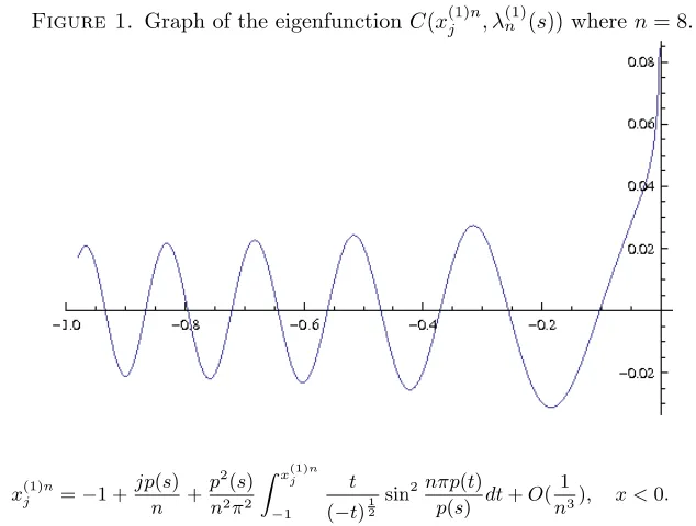
In Figure 1, we illustrate graph of the eigenfunction C(x(1)_j n, λ(1)n (s)) where n = 8,−1 ≤

x <0.

Using (2.14), we obtain

Figure 1. Graph of the eigenfunctionC(x(1)j n, λ

(1)

n (s)) wheren= 8.

x(1)j n=−1 +

jp(s) n +

p2(s) n2_π2

Z x(1)n_j

−1 t (−t)12

1

n3), x <0.

(12)

Table 2. Detailed results for the nodal points ofx(2)j nwherej= 1,8

andn= 1,8.

x(2)n_j j=1 j=2 j=3 j=4 j=5 j=6 j=7 j=8 n=1 0.967396

n=2 0.565054 0.994646

n=3 0.419539 0.738236 0.997899

n=4 0.341553 0.600941 0.812288 0.998887

n=5 0.291896 0.513548 0.69415 0.853605 0.999312

n=6 0.257053 0.452236 0.611272 0.751686 0.879995 0.999533

n=7 0.231028 0.406443 0.549374 0.675568 0.790883 0.898316 0.999663

n=8 0.210721 0.370714 0.501079 0.616179 0.721355 0.819343 0.91178 0.999745

We can obtain the eigenfunction of this problem as

C(x, λ(2)n (s)) =

x−14_e 2 3(

nπ−π 4

f(s) )_cos[_f₍_x₎₍nπ− π 4

f(s) )−

π

4]

(nπ−π4

f(s) )

+x

−1 4e

2 3(

nπ−π₄

f(s) )

nπ−π 4

f(s)

sin[f(x)(nπ− π

4 f(s) )−

π 4]

Z x

0

t12_cos2_[_f₍_t₎₍nπ−

π

4 f(s) )−

π

4]dt+O( 1

n3). (4.1)

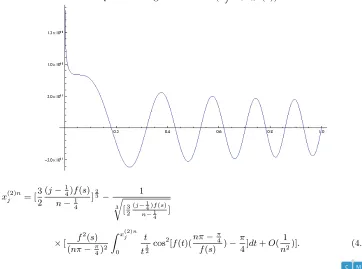
In Figure 2, we illustrate graph of the eigenfunctionC(x(2)_j n, λn(2)(s)) wheren= 8, 0≤x <1. Using (2.16), we obtain

Figure 2. Graph of the eigenfunctionC(x(1)j n, λ

(2)

n (s)) wheren= 8.

x(2)_j n= [3 2

(j−1 4)f(s) n−1

4

]23₋ 1

3

r

[3₂(j−

1 4)f(s)

n−1 4

]

×[ f

2₍_s₎

(nπ−π

4) 2

Z x(2)n_j

0 t

t12

cos2[f(t)(nπ− π

4 f(s) )−

π

4]dt+O( 1

(13)

5. Conclusions

In this study, the nodal points were used to solve the inverse Sturm-Liouville problem with a turning point. In the numerical examples, we have shown that the obtained nodes correspond to the roots of eigenfunction. Then we calculated the solution of inverse problem by using the nodal points.

References

[1] A. J. Akbarfam, Higher-order asymptotic approximations to the eigenvalues of the Sturm-Liouville problem in one turning point case, AJSE., 24 (1999), 1A, January. DOI 10.1137/S0036142994264882.

[2] A. J. Akbarfam and E. Pourreza,A Research note on the second order differential equation, J. Sci. I. R. Iran.,10(3) (1999), 185–192.

[3] A. J. Akbarfam and A. B. Mingarelli, The canonical product of the solution of the Sturm-Liouville equation in one turning point case, Canad. Appl. Math. Quart.,13(4) (2000), 305–320. [4] V. A. Ambarzumyan,Uber eine frage der eigenwerttheorie¨ , Z. Phys.,53(1929), 690–695. [5] G. Borg,Eine umkehrung der Sturm-Liouvillesehen eigenwertaufgabe, Acta Math.,78(1945),

1–96.

[6] S. A. Buterin and C. T. Shieh,Incomplete inverse spectral and nodal problems for differential pencils, Results. Math. ,62(2012), 167–179.

[7] A. Dabbaghian and A. Neamaty, On the determination of asymptotic formula of the nodal points for the Sturm-Liouville equation with one turning point, Caspian Journal of Mathematical Sciences.,3(1) (2014), 175–181.

[8] W. Eberhard, G. Freiling, and A. Schneider,Connection formulae for second-order differential equations with a complex parameter and having an arbitrary number of turning points, Geophys. J. R. Astr. Soc.,50(1997), 303–309.

[9] G. Freiling and V. A. Yurko, Inverse problems for differential equations with turning points, Inverse Problems.,13(1997), 1247–1263.

[10] G. Freiling and V. A. Yurko,Inverse Sturm-Liouville Problems and Their Applications. Nova Science Publishers, New York, 2001.

[11] A. L. Goldenveizer, V. B. Lidsky, and P. E. Tovstik,Free vibration of thin elastic shells, Nauka, Moscow, 1979.

[12] H. Koyunbakan and E. S. Panakhov,Inverse problem for a singular differential operator, Math-ematical and Computer Modelling.,47(2008), 178–185.

[13] H. Koyunbakan,A new inverse problem for the diffusion operator, Appl. Math. Lett.,19(2006), 995–999.

[14] C. K. Law, C. L. Shen, and C. F. Yang,The inverse nodal problem on the smoothness of the potential function, Inverse Problems. ,15(1999), 253–263.

[15] B. M. Levitan,On the determination of the Sturm-Liouville operator from one and two spectra, Mathematics of the USSR Izvestija.,12(1978), 179–193.

[16] V. A. Marchenko,Certain problems of the theory of one dimensional linear differential operators of the second order 1, Tr. Mosk. Mat. Obs.,1(1952), 327–340.

[17] V. A. Marchenko, Sturm-Liouville operators and their applications, Naukova Dumka, Kiev, 1977; English transl., Birkhuser, 1986.

[18] J. Mc Hugh,An historical survey of ordinary linear differential equations with a large parameter and turning points, Arch. Hist. Exact Sci.,7(1970), 277–324.

[19] J. R. McLaughlin,An inverse spectral theory using nodal points as a data-a uniqueness result, J. differential Equations.,73(1988), 354–362.

[20] J. D. Murray,Asymptotic analysis, Springer-Verlag, New York, 1973.

[21] A. Neamaty and S. Mosazadeh, On the canonical solution of Sturm-Liouville problem with singularity and turning point of even order, Canad. Math. Bull.,54(3) (2011), 506–518. [22] C. T. Shieh and V. Yurko,Inverse nodal and inverse spectral problems for discontinuous

(14)

[23] Y. P. Wang, C. F. Yang, and Z. Y. Huang,Half inverse problem for Sturm-Liouville operators with boundary conditions dependent on the spectral parameter, Turkish J. Math.,37(3) (2013), 445–454.