Ecosystem function and particle flux dynamics across the Mackenzie Shelf (Beaufort Sea, Arctic Ocean): an integrative analysis of spatial variability and biophysical forcings

Biogeosciences, 10, 2833–2866, 2013 www.biogeosciences.net/10/2833/2013/ doi:10.5194/bg-10-2833-2013

© Author(s) 2013. CC Attribution 3.0 License.

Advances in

Geosciences

Open Access

Natural Hazards

and Earth System

Sciences

Open Access

Annales

Geophysicae

Open Access

Nonlinear Processes

in Geophysics

Open Access

Atmospheric

Chemistry

and Physics

Open Access

Atmospheric

Chemistry

and Physics

Open Access

Discussions

Atmospheric

Measurement

Techniques

Open Access

Atmospheric

Measurement

Techniques

Open Access

Discussions

Biogeosciences

Open Access Open Access

Biogeosciences

Climate

of the Past

Open Access Open Access

Climate

of the Past

Discussions

Earth System

Dynamics

Open Access Open Access

Earth System

Dynamics

Discussions

Geoscientific

Instrumentation

Methods and

Data Systems

Open Access

_{Geoscientific}

Instrumentation

Methods and

Data Systems

Open Access

Discussions

Geoscientific

Model Development

Open Access Open Access

Geoscientific

Model Development

Hydrology and

Earth System

Sciences

Open Access

Hydrology and

Earth System

Sciences

Open Access

Discussions

Ocean Science

Open Access Open Access

Ocean Science

Discussions

Solid Earth

Open Access Open Access

Solid Earth

The Cryosphere

Open Access Open Access

The Cryosphere

Discussions

Natural Hazards

and Earth System

Sciences

Open Access

Discussions

Ecosystem function and particle flux dynamics across the Mackenzie

Shelf (Beaufort Sea, Arctic Ocean): an integrative analysis of spatial

variability and biophysical forcings

A. Forest1, M. Babin1, L. Stemmann2, M. Picheral2, M. Sampei3, L. Fortier1, Y. Gratton4, S. B´elanger5, E. Devred1,

J. Sahlin1, D. Doxaran2, F. Joux6,7, E. Ortega-Retuerta6,7,8, J. Mart´ın8,10, W. H. Jeffrey9, B. Gasser10, and

J. Carlos Miquel10

1_{Takuvik Joint International Laboratory, UMI 3376, Universit´e Laval (Canada) – CNRS (France), D´epartement de Biologie} and Qu´ebec-Oc´ean, Universit´e Laval, Qu´ebec G1V 0A6, Canada

2_{UPMC Universit´e Paris 06, UMR 7093, Laboratoire d’Oc´eanographie de Villefranche 06230, Villefranche-sur-Mer, France} 3_{Graduate School of Biosphere Science, Hiroshima University, Higashi Hiroshima 739-8511, Japan}

4_{Institut National de la Recherche Scientifique – Eau Terre Environnement, Qu´ebec G1K 9A9, Canada}

5_{D´epartement de Biologie, Chimie et G´eographie, Universit´e du Qu´ebec `a Rimouski, Rimouski, Qu´ebec G5L 3A1, Canada} 6_{UPMC Universit´e Paris 06, UMR 7621, Laboratoire d’Oc´eanographie Biologique de Banyuls, Observatoire Oc´eanologique,} 66650 Banyuls-sur-Mer, France

7_{CNRS, UMR 7621, Laboratoire d’Oc´eanographie Microbienne, Observatoire Oc´eanologique, 66650 Banyuls-sur-Mer,} France

8_{Instituto de Ciencias del Mar (CSIC). Paseo Mar´ıtimo de la Barceloneta, 37-49, 08003 Barcelona, Spain}

9_{Center for Environmental Diagnostics and Bioremediation, University of West Florida, Pensacola FL-32514, USA} 10_{IAEA Environment Laboratories, MC98000, Monaco, Monaco}

Correspondence to: A. Forest (alexandre.forest@takuvik.ulaval.ca)

Received: 24 July 2012 – Published in Biogeosciences Discuss.: 14 August 2012 Revised: 22 March 2013 – Accepted: 1 April 2013 – Published: 2 May 2013

Abstract. A better understanding of how environmental changes affect organic matter fluxes in Arctic marine ecosys-tems is sorely needed. Here we combine mooring times se-ries, ship-based measurements and remote sensing to assess the variability and forcing factors of vertical fluxes of par-ticulate organic carbon (POC) across the Mackenzie Shelf in 2009. We developed a geospatial model of these fluxes to proceed to an integrative analysis of their determinants in summer. Flux data were obtained with sediment traps moored around 125 m and via a regional empirical algo-rithm applied to particle size distributions (17 classes from 0.08–4.2 mm) measured by an Underwater Vision Profiler 5. The low fractal dimension (i.e., porous, fluffy particles) de-rived from the algorithm (1.26±0.34) and the dominance (∼77 %) of rapidly sinking small aggregates (<0.5 mm) in total fluxes suggested that settling material was the product of recent aggregation processes between marine detritus,

by diatoms. Among biophysical parameters, bacterial pro-duction and northeasterly wind (upwelling-favorable) were the two strongest corollaries of POC fluxes (r2cum.=0.37). Bacteria were correlated with small aggregates, while north-easterly wind was associated with large size classes (>1 mm ESD), but these two factors were weakly related with each other. Copepod biomass was overall negatively correlated (p<0.05) with vertical POC fluxes, implying that metazoans acted as regulators of export fluxes, even if their role was mi-nor given that our study spanned the onset of diapause. Our results demonstrate that on interior Arctic shelves where pro-ductivity is low in mid-summer, localized upwelling zones (nutrient enrichment) may result in the formation of large fil-amentous phytoaggregates that are not substantially retained by copepod and bacterial communities.

1 Introduction

The magnitude and nature of particulate organic carbon (POC) fluxes in marine ecosystems are key indices of biolog-ical productivity and ecosystem functioning (e.g., Longhurst et al., 1989; Wassmann, 1998; Boyd and Trull, 2007). Down-ward POC fluxes drive the transfer of energy from the sunlit surface layer to benthic organisms and eventually support the sequestration of atmospheric carbon dioxide (CO2)in marine sediments (Honjo et al., 2008). In regions close to the con-tinental shelf, resuspension and lateral advection processes that transport POC from the shelves to the deep basins are additional mechanisms that facilitate the long-term storage of CO2at depth (Hwang et al., 2010). Conversely, trophic in-teractions in planktonic food webs keep cycling organic mat-ter in the pelagic environment, move energy toward verte-brates, and ultimately return POC back to atmospheric CO2 through respiration (e.g., Forest et al., 2011). Understanding the spatial–temporal variability and physical–biological de-terminants of organic matter fluxes is therefore crucial to bet-ter resolve processes structuring marine food webs and con-trolling the biological pumping of CO2by the ocean biota. This is particularly true as rising CO2and associated global warming progressively alter physical and chemical parame-ters of the water column (e.g., temperature, freshwater con-tent, pH, etc.) and modify various biological properties such as plankton metabolism, size distribution, and trophic inter-actions (Doney et al., 2012). Changes in the lower food web have implications for biogeochemical cycling and feedback to the climatic machinery (e.g., Steinberg et al., 2012) and might directly impact ecosystem services upon which people depend for their subsistence and economic wellbeing.

A better comprehension of particle flux dynamics in rela-tionship with ecosystem functioning is particularly needed in Arctic marine ecosystems where rapid environmental changes induced by the combination of both anthropogenic and natural forcings currently occur (ACIA, 2005; IPCC,

broad spatial structures was performed using the principal coordinate of neighbor matrices method (PCNM; Borcard et al., 2004). Assessment of relationships between physical– biological variables, spatial–temporal trends and vertical flux size classes (i.e., used as “species”) was conducted using redundancy analyses (RDAs), forward selection procedures, and variation partitioning. Our statistical analyses enabled us to test an exhaustive suite of hypotheses regarding the con-trol and variability of vertical POC fluxes across the Arctic shelf-basin system.

2 Material and methods

2.1 Physical and biological setting of the study area

Seasonal sea ice over the Mackenzie Shelf (Fig. 1) reaches a maximum thickness of∼2–3 m in March–April and is usu-ally melted by mid-September (Barber and Hanesiak, 2004). The shelf is influenced by the Mackenzie River, which brings a large volume of freshwater (330 km3yr−1)and sediment load (124 ×106t yr−1), primarily between May and Septem-ber (Gordeev, 2006). During summer, ice melt and river runoff generate a highly stratified surface layer in the top 5– 10 m of the water column (Carmack and Macdonald, 2002). Water masses in the region come from various sources and comprise the following: sea ice melt water, the Mackenzie River, the winter polar mixed layer (above∼50 m), summer and winter water of Pacific origin (∼50–200 m), Atlantic water (∼200–800 m), and Canada Basin deep water (below 800 m depth) (Lansard et al., 2012). Surface ocean circula-tion in the region is complex and largely influenced by wind and sea ice conditions (Ingram et al., 2008). Inshore, a typ-ical coastal current flows from the west to the east. North-westerly winds tend to retain surface waters inshore (down-welling conditions), whereas easterlies push them seaward (upwelling conditions) (Macdonald and Yu, 2006). The dis-tance of the ice edge from the shelf break strongly influences the strength of the upwelling/downwelling flow (Carmack and Chapman, 2003). Offshore, surface circulation is over-all driven by the anticyclonic Beaufort Gyre, while below the surface layer, circulation is reversed and dominated by the eastward Beaufort Undercurrent carrying waters of both Pacific and Atlantic origin along the slope (Ingram et al., 2008). A narrow shelf break jet (20 km width, centered at 100–200 m depth) appears to be an inherent structure of the subsurface countercurrent (Pickart, 2004).

Primary production in the Beaufort Sea is low when com-pared with other Arctic shelves and typically ranges from 30 to 70 g C m−2yr−1(Sakshaug, 2004; Carmack et al., 2004). The spring bloom rapidly evolves into a subsurface chloro-phyll maximum (SCM) that progressively lowers the nitr-acline over the growth season (Martin et al., 2010). The injection of deep nutrients into the surface layer through

141°W _138°W

135°W 132°W 129°W 126°W

Depth (m)

50 100 250 500 750 1000

25

Sampling date 1 Aug

18 Jul 15 Aug

72°N

71°N

70°N

69°N

Tuktoyaktuk Peninsula

Cape Bathurst

Amundsen Gulf

Mackenzie River Mackenzie

Trough Franklin Bay

Kugmallit Valley

Mackenzie Delta

CA05

CA16 Line 100

Mackenzie

Shelf G09

A1

Canada Basin

Line 200 Line

400 Line 500

St. 345 Line 300

Line 600 Line 700

North America Arctic Ocean

Oceanographic stations

Long-term moorings Drifting sediment traps

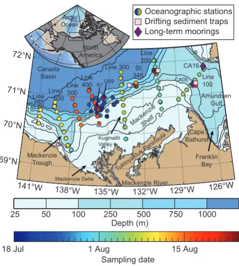
Fig. 1. Bathymetric map of the southeast Beaufort Sea (Arctic Ocean) with position of the sampling stations conducted in July– August 2009 as part of the ArcticNet-Malina campaign. The Arc-ticNet sampling sites were located in the exploration license area EL446, whereas transects 100–700 and station 345 correspond to the Malina sampling grid. On each Malina transect, station IDs are numbered in increasing number from north to south (e.g., 110 to 170 from north to south on line 100). The position of short-term (ca. 24 h) and long-term (ca. 1 yr) deployments of automated sed-iment traps is also indicated on the map. Technical details on the short-term drifting traps and long-term moorings can be found in Table 1. A 3-D interactive visualization of the bathymetric domain of southeast Beaufort Sea is also accessible through the online Sup-plement (see Appendix C for details).

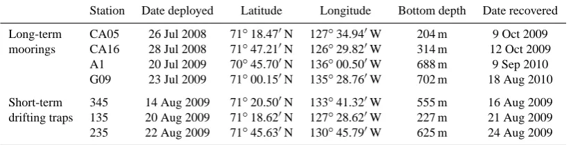
Table 1. Locations and periods of deployment of the long-term moorings and short-term drifting traps used in the present study. The location of each station is mapped on Fig. 1.

Station Date deployed Latitude Longitude Bottom depth Date recovered

Long-term CA05 26 Jul 2008 71◦18.470N 127◦34.940W 204 m 9 Oct 2009 moorings CA16 28 Jul 2008 71◦47.210N 126◦29.820W 314 m 12 Oct 2009 A1 20 Jul 2009 70◦45.700N 136◦00.500W 688 m 9 Sep 2010 G09 23 Jul 2009 71◦00.150N 135◦28.760W 702 m 18 Aug 2010

Short-term 345 14 Aug 2009 71◦20.500N 133◦41.320W 555 m 16 Aug 2009 drifting traps 135 20 Aug 2009 71◦18.620N 127◦28.620W 227 m 21 Aug 2009 235 22 Aug 2009 71◦45.630N 130◦45.790W 625 m 24 Aug 2009

2.2 Atmospheric conditions, sea ice, and river discharge

Mean daily wind and pressure data at surface (0.995 sigma level, 2.5◦ _×2.5◦ _{resolution) were obtained from the}

Na-tional Centers for Environmental Prediction (NCEP) Re-analysis project (Kalnay et al., 1996) available online (http: //www.esrl.noaa.gov/psd/). NCEP wind and pressure data were favored over measurements made at coastal weather stations (e.g., Tuktoyaktuk) because of uncertainties related to the presence of land (Williams et al., 2006). Wind and pressure data were spatially averaged for the whole study re-gion (69.5–72◦N, 126–141◦W, Fig. 1) in order to produce an annual time series for the year 2009. A 7-day recent history of average wind conditions was also produced for every near-est 2.5◦×2.5◦ pixel corresponding to each oceanographic station conducted during the ArcticNet-Malina campaign (Fig. 1). These wind data were adjusted (50°anticlockwise) to produce along-shelf (northeasterly) and cross-shelf (south-easterly) wind vectors that are favorable to shelf break up-welling (Ingram et al., 2008).

Daily averaged sea ice concentrations (% of coverage) across the Mackenzie Shelf region were obtained from the Special Sensor Microwave Imager (SSM/I) located onboard the DMSP satellite. Daily maps were processed by the Ifremer-CERSAT Team (http://cersat.ifremer.fr/) using the daily brightness temperature maps from the National Snow and Ice Data Center (Maslanik and Stroeve, 1999). The Artist sea ice algorithm (Kaleschke et al., 2001) was used to process daily sea ice concentration maps at 12.5 km resolution. Sea ice concentrations were averaged for the whole study area in order to produce a time series of sea ice conditions in 2009 compared with 1998–2008. A 15-day history of mean sea ice concentration (37.5×37.5 km) was also produced for each station conducted during the summer 2009 expedition (Fig. 1).

Mean daily water discharge from the Mackenzie River (station Arctic Red River, 10LC014) was obtained from the Water Survey of Canada (http://www.wsc.ec.gc.ca/ applications/H2O/). We used data from Arctic Red River as it represents roughly 94 % of the total Mackenzie catch-ment and corresponds to the most downstream station before

the Mackenzie River splits into many channels in the delta (Leitch et al., 2007). A time series of Mackenzie River wa-ter discharge was constructed for the year 2009 to be used in comparison with the mean discharge from 1998 to 2008.

2.3 Satellite remote sensing of surface POC

concentrations

A time series of 290 level-1b satellite images (free or partly free of clouds) of the Mackenzie Shelf region col-lected with the Medium Resolution Imaging Spectrome-ter (MERIS) onboard the Envisat platform over the period of May–September 2009 were acquired from the ODESA website (http://earth.eo.esa.int/odesa/). All images were pro-cessed to level 2 with the ODESA CFI software and using the alternative atmospheric correction of Babin and Mazeran (2010). For more information about the standard process of MERIS level-2 products, please see ESA (2011). Monthly (May, September) and semi-monthly (June–August) com-posites of MERIS images (1 km resolution) were gener-ated using the mosaic algorithm of the Beam/VISAT open-source software (http://www.brockmann-consult.de/beam/). The sea ice adjacency mask of B´elanger et al. (2007) to de-tect pixels potentially contaminated by the presence of sea ice was implemented in the mosaicking processing chain. A regional POC algorithm based on the empirical relation-ship between in situ surface POC concentration and the blue-to-green ratio of remote-sensing reflectance (490, 560 nm) measured during the Canadian Arctic Shelf Exchange Study (CASES) 2004 and Malina 2009 field campaigns was applied to level-2 images during the process. For a complete method-ology on the development of the regional POC algorithm, see Appendix B.

traps

Four long-term mooring lines (bottom-anchored) equipped with automated sediment traps at∼100 and / or∼200 m depth (Technicap PPS 3/3 cylindrico-conical trap, 0.125 m2 aperture, aspect ratio of 2.5 in their cylindrical part) were de-ployed across the Mackenzie Shelf region during 2009 (Ta-ble 1, Fig. 1). All moorings were equipped with conductiv-ity/temperature sensors (RBR CT or JFE ALEC) and acous-tic doppler current profilers (Nortek or Teledyne) to record basic physical properties and oceanic circulation at various depths throughout the water column. Only mooring CA05 (Fig. 1) was equipped with a complete suite of bio-optical sensors: photosynthetic available radiation (PAR) at 54 m (JFE ALEC ALW), chlorophyll a (Chl a)fluorescence at 54 m (JFE ALEC CLW), as well as turbidity at 54 m (JFE ALEC CLW), 57 m (Seapoint), and 178vm (AADI). Moor-ing CA05 was also the only observatory equipped with an Aanderaa RCM-11 multisensors located ∼ 20 m above the seafloor to monitor current speed, direction, temperature, salinity, and turbidity close to the benthic boundary layer. Current-meter data were filtered using the pl64 low-pass fil-ter (Alessi et al., 1985) to remove the tidal signal. Current components (U, V) and bio-optical sensor data were then av-eraged over daily periods.

During the Malina field campaign, a drifting line equipped with an array of automated sediment traps (Technicap PPS 3/3, same traps as on long-term moorings) was deployed at 3 sites across the region (Table 1, Fig. 1). Given the rela-tively high weight of each trap in water (17 kg), drifting lines were equipped with an adequate series of Viny and Nokalon floats to ensure suitable floatability. The use of sequential traps in such drifting mode has been successfully tested in various environments (e.g., Peinert and Miquel, 1994; Guidi et al., 2008). For each deployment, the length of the mooring line, number of instruments, and sampling intervals had to be adapted to the constraints imposed by bottom depth, ice cover and survey schedules. The first deployment took place from 14–16 August at station 345. Four traps were installed at depths of 45, 90, 150, and 200 m. The total sampling time spanned for 32 h, divided into two 16 h intervals. The sec-ond deployment took place from 20 to 22 August at station 135. Three traps were deployed at 40, 85, and 150 m depth for 28 h, in two intervals of 14 h each. The third deployment took place at station 235 from 22 to 24 August. Four traps were attached to the drifting line at 40, 85, 145, and 200 m depth respectively. A single sample (50 h) was retrieved per trap. Given the limited amount of settling mass flux in all cases, the two sequential samples in deployments first and second were merged in a single filter in order to obtain reli-able results.

Before deployments, sediment traps for both long-term and short-term deployments were prepared following the JGOFS protocol (Knap et al., 1996). The traps’ sample cups

salinity with NaCl. Formalin was added for preservation (5 % v/v, sodium borate buffered) to prevent grazing by zooplank-ton and remineralization of organic matter. No brine to fill the whole sediment trap was added in any of the short-term or long-term collection. After retrieval, cups were checked for salinity and put aside 24 h to allow particles to settle. Sam-ples were stored at 4 °C until they were processed.

Analyses of long-term mooring samples were performed at Universit´e Laval (Canada) whereas drifting trap sam-ples were processed at the IAEA Environment Laboratories (Monaco). In all samples, “swimmers” (zooplankton deemed to be alive at the time of collection) were handpicked from the samples with forceps under a stereomicroscope. Micro-scopic analyses to discriminate the contribution of zooplank-ton carcasses to the sinking flux (Sampei et al., 2009) will be presented elsewhere. Particle samples were divided into several subsamples with a Motoda splitting box (Canada) or a McLane Wet Samples Divider (Monaco). Long-term sedi-ment trap subsamples were filtered through preweighed GF/F filters (25 mm, precombusted at 450 °C for 3 h), desalted with freshwater, and dried for 12 h at 60 °C for the determination of dry weight (DW). The subsamples were exposed for 12 h to concentrated HCl fumes to remove the inorganic carbon fraction. Samples were analyzed on a CHN Perkin Elmer 2400 Series II to measure POC fluxes. Different fractions of short-term trap samples were processed and stored apart for other analyses than DW and POC, whose results will be presented elsewhere. A 40 % fraction was used for DW and POC analyses. This fraction was desalted and vacuum-filtered unto precombusted QMA 25 mm filters. The filters were dried at 40 °C overnight, left 24 h in a desiccator to stabilize at room temperature and then weighted to obtain mass flux. To obtain the organic carbon content (as % of dry weight), filters were decalcified with 1 M H3PO4and ana-lyzed in an Elementar Vario EL autoanalyzer. Several runs of blanks (precombusted QMA filters) and standards (Ac-etanilide Merck pro analysis) were also performed for cal-ibration of carbon measurements.

2.5 Ship-based measurements of physical and biological

variables

p<0.01,n=48). The two equations were linked to a change in the gain of the Seapoint fluorometer during the field cam-paign. Data from the CTD, fluorometer and transmissometer from all casts were averaged over 1 m bins.

The rosette profiler was also equipped with an Underwa-ter Vision Profiler 5 (UVP5) allowing routine recordings of particle size distributions (i.e., both nonliving particles and zooplankton). Full details of the technical specifications and processing operations of the UVP5 can be found in Picheral et al. (2010) and in Forest et al. (2012). Briefly, the UVP5 aims at recording and measuring all objects>80 µ m ESD (i.e., inferior limit of the lowest size class) in real time dur-ing deployment. The size and grey level of every object are calculated in situ, but only images of objects>600 µ m are stored on a memory stick for further processing. The Zoopro-cess imaging software (http://www.zooscan.com) was used to identify major zooplankton groups (>600 µm) with the Plankton Identifier (PkID) (Gorsky et al., 2010). The predic-tion of organisms obtained from the PkID files was exhaus-tively post-validated to obtain an accurate dataset of abun-dance and biovolume for zooplankton larger than 600 µ m from the UVP5. The zooplankton dataset acquired with the UVP5 during the ArcticNet-Malina campaign was further compared with zooplankton collected in situ with 29 verti-cal net tows, which showed very good agreement (see Forest et al., 2012 for details). This enabled us to use the zooplank-ton biovolume dataset obtained with the UVP5 to estimate zooplankton biomass over a fine-scale spatial grid.

Zooplankton biovolume was converted into carbon biomass using various conversion factors gathered from the literature. We are confident that the use of the UVP5 dataset provided reliable estimate of zooplankton biomass since large organisms dominate this biomass in the Beaufort Sea (e.g., Darnis et al., 2008; Forest et al., 2011). For copepods we used the regional relationship established by Forest et al. (2012). For appendicularians, ctenophores, chaetognaths, and other gelatinous organisms, we used the conversion fac-tors of Lehette and Hernandez-Leon (2009) assuming a 30 % carbon content in the DW of appendicularians and medusae (Deibel, 1986; Larson, 1986) and a 50 % carbon content in the DW of chaetognaths (Baguley et al., 2004). For proto-zoans we used the mean conversion factor for foraminifers and radiolarians of Michaels et al. (1995).

Exhaustive measurements of bacterial production (BP) were conducted throughout the ArcticNet-Malina expedition (Ortega-Retuerta et al., 2012a) with the classical3H-leucine incorporation method (Kirchman, 2001). Briefly, samples (1.5 ml in triplicates) were incubated for 2 h at in situ tem-perature with 10–20 nM of [4,5-3H]-leucine (specific activ-ity 139 Ci mmole−1, Amersham). Incubations were termi-nated by adding trichloroacetic acid (TCA, 5 % final concen-tration). The incorporated3H leucine was collected by mi-crocentrifugation and rinsed once with 5 % TCA and once with 70 % ethanol before radioassaying (Ortega-Retuerta et al., 2012a). A conversion factor of 1.2 kg C per mole of

leucine was used to transform3H-leucine incorporation into carbon production, following the rationale of a recent work on planktonic carbon flows in the Beaufort Sea (Forest et al., 2011). It should be noted that BP in the present study represents the production by the total community, including both free-living and particle-attached bacteria (see Ortega-Retuerta et al., 2012b, c for details).

2.6 Optimization procedure and statistical analyses

In order to obtain vertical particle fluxes at a fine spatial scale during the field campaign, we computed a regional algorithm linking the particle size distributions recorded by the UVP5 (0.08–4.2 mm ESD) to mass and POC fluxes estimated by the sediment traps at overlapping sampling locations and pe-riods. When more than one UVP5 deployment corresponded to only one sediment trap sample (mainly for long-term traps; see Fig. A1a), the abundance of particles for each size class for all corresponding profiles were averaged. A sensitivity test to document the degree of confidence in our approach was also conducted using a multiple random resampling of our database (Appendix A, Fig. A1b). The identifiable zoo-plankton dataset (≥ 0.6 mm ESD) was removed from the UVP5 particle database before proceeding to the computa-tion of the regional algorithm. The optimizacomputa-tion procedure of Guidi et al. (2008) making use of the Matlab function

fmin-search (MathWorks, USA) was adapted to our dataset to find

theAandbvalues that minimized the log-transformed dif-ferences between sediment trap data (mass and POC) and the spectrally estimated mass or POC fluxes in the following power-law equation:

F =

4.2

Z

0.08

n·A·db, (1)

whereF is the flux integrated from 0.08–4.2 mm ESD (mass or POC, in mg m−2d−1,nis the concentration of particles in a given size class (# L−1, or # 10−3m−3),Ais a constant (mg m1−bd−1),dis the mean ESD of particles in a given size class (mm, or 10−3m), andbis the scaling exponent of the power-law relationship (no unit). On the basis of the scal-ing exponentb, the mean fractal dimension (D, unitless) of particles (e.g., Jackson and Burd, 1998; Li and Logan, 2000; Guidi et al., 2008) along the size spectrum can be easily cal-culated using the equation

D=b+1

2 . (2)

at the same spatial and temporal resolution than the UVP5 dataset (including a set of spatial structures; see below). We could obtain 12 physical–biological constraints for our sta-tistical analyses: 2 near-history wind components, sea ice persistence, water column density (σθ), bottom depth,

sur-face POC concentration, mean beam attenuation coefficient, Chla inventory, bacterial production, and 3 groups of zoo-plankton (copepods, appendicularians and others; see Forest et al., 2012). The RDAs were followed by the forward se-lection of reduced models of only significant relationships and a variation partitioning analysis (Borcard et al., 2011 and references therein). All RDAs were plotted as symmetri-cally scaled by the square root of eigenvalues (i.e., scaling=

3; Oksanen, 2011) and station ordination scores were given as weighted sums of the species scores to show the overall variability for both sites and size classes. Prior to analysis, POC fluxes were log-transformed to give equal weights to all size classes. All analyses were conducted using the R free-ware (http://www.r-project.org/) with the appropriate pack-ages (Borcard et al., 2011).

Spatial structures of POC fluxes across the Mackenzie Shelf were obtained using the principal coordinates of neigh-bor matrices (PCNM) procedure. The goal of the PCNM method is to identify patterns and gradients across a whole range of fine-to-broad scales (2-D) perceptible within a given dataset (Borcard et al., 2004). This procedure generates a suite of variables that can readily be used in further analyses, such as RDAs and variation partitioning (e.g., Peres-Neto et al., 2006). When used on an irregular sampling design – such as in the present analysis – the PCNM functions corre-spond to irregular sinusoidal-like waveforms, within which spatial structures along the X-Y geographic coordinates are repeated. The scale of every PCNM function is zero-centered on the mean and is a measure of the recurrent spatial struc-ture, so that the value of each station (i.e., positive or nega-tive) provides its fitted position on the waveform (e.g., Bor-card et al., 2004). Briefly, the PCNM orthogonal variables are obtained through the following: (1) the construction of an Euclidean distance matrix among station sites, (2) the trunca-tion of this matrix to retain distances among close neighbors based on a threshold corresponding to the longest distance along the spanning tree drawn on the station map, (3) the computation of a principal component analysis of the trun-cated distance matrix, and (4) the retention of the PCNM functions that model a positive spatial correlation of Moran’s

I (Moran, 1950). Because the goal of the present study was

to include PCNM functions as part of a variation partition-ing analysis, POC flux data were not detrended, as advocated by Borcard et al. (2011). Hence, the pure linear trend due to sampling date and location was incorporated in the variation partitioning that aimed at quantifying the unique and com-bined fractions of variation explained by numerous sources.

3.1 Environmental conditions and surface POC

concentrations

Atmospheric pressure and wind conditions over the Macken-zie Shelf region varied markedly throughout 2009 (Fig. 2a). The yearly average surface pressure field yielded a value of 0.99 atm, and the annual mean wind vector was estimated as a weak easterly wind of 2.4 m s−1. Sea ice concentrations in 2009 were near the average of 1998–2008 (Fig. 2b), but it should be noted that a high standard deviation was associ-ated with the latter mean in the summer months (±30 % in June,±24 % in July, and±16 % in August; not shown). In fact, ice conditions in the Beaufort Sea were more severe in 2009 than during the previous 5 years when intensive sam-pling occurred as part of the CASES-ArcticNet expeditions and Circumpolar Flaw Lead (CFL) System Study.

Persistent northerly/northeasterly winds blew at an aver-age speed of 5 m s−1throughout much of the month of July prior to the field campaign (Fig. 2a). This resulted in a steady southward advection of the central ice pack visible in the satellite images of July (Fig. 3) and mirrored in the above-average ice concentration observed in late July (Fig. 2b). The wind pattern broke up in August and winds blowing from the south dominated in late summer. A steady decline from high to low atmospheric pressure was concomitantly recorded from early July to September (Fig. 2a), which brought cloudy conditions during the Malina campaign, especially during the second half of August, as revealed by the numerous white patches in Fig. 3 (panel 15–29 August). The southerly winds in August contributed to poleward ice motion and ice melt across the study area (Fig. 2b, Fig. 3).

Atmospheric

pressure (atm)

10

5

0

10 5

1.000

0.970 1.030

50

25

0 75 100

10

0 20 30

Wind speed

(m s

-1)

Sea ice

concentration (%)

River discharge (x10 3 m 3 s -1)

2009

Mean 1998-2008

2009

Mean 1998-2008

North Atm. press.

(a)

(b)

(c)

1.015

0.985

Jan Feb Mar Apr May Jun Jul Aug Sept Oct Nov Dec

ArcticNet-Malina

Fig. 2. Time series from January to December 2009 of (a) near-surface wind vectors and atmospheric pressure (source: NCEP); (b) daily ice concentration and recent decadal average (source: NSIDC); and (c) daily Mackenzie River discharge and decadal mean (as recorded at station Arctic Red River). Data from panels a–b correspond to regional averages over the entire southeast Beaufort Sea as defined as the area shown in Fig. 1. The gray-shaded column indicates the temporal window within which the ArcticNet-Malina campaign was conducted.

3.2 Mooring-based measurements and drifting

short-term traps

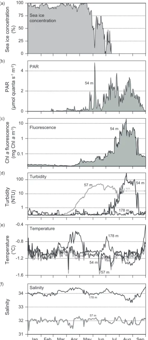
Physical and bio-optical parameters measured from January to September 2009 at mooring CA05 provided informa-tion on the seasonal variability of pelagic condiinforma-tions in the southeast Beaufort Sea prior to the summer field campaign (Figs. 4, 5). Light available (PAR) at 54 m remained close to nil values until late May consistently with sea ice con-centrations that ranged from 90 to 100 % during this period (Fig. 4a, b). Light in the upper water column during the melt period was sensitive to oscillation in sea ice concentration as an apparent negative correlation was observed between sea ice and PAR from late May to late July (Fig. 4a). PAR de-creased roughly twofold in early August, when fluorescence at the same depth rose above ∼ 1 mg Chlam−3 (Fig. 4b, c). Turbidity recorded with the JFE ALEC CLW at 54 m (same sensor as fluorescence) showed a quasi-parallel trend as Chlafluorescence. Interestingly, turbidity measured with the Seapoint sensor a 57 m depth exhibited an earlier rise (May) than the turbidity recorded with the CLW (July), but measurements with the Seapoint in mid-August–September were hindered by sensor fouling. Turbidity at 178 m re-mained low (<1 NTU) throughout the duration of the de-ployment (Fig. 4d). Temperature monitored at 54, 57, and 178 m at CA05 stayed below 0 °C from January to Septem-ber (Fig. 4e). Such a relative homogeneity of temperature at discrete depths in the upper water column could be in-dicative of well-mixed conditions, but the salinity time series (Fig. 4f) rather demonstrates that the water column was

con-tinuously stratified. In fact, temperature in the core of the Pacific-derived water mass (∼100 m) in the Beaufort Sea is commonly near−1.6 °C.

Variation in the intensity and direction of the water flow recorded at various depths at mooring CA05 over January to September 2009 was pronounced (Fig. 5). Direction of current vectors followed overall an along-shelf axis, follow-ing the bathymetry. Strongest currents (up to 35 cm s−1 at 22 m depth) were detected in late winter, when the ice cover was apparently consolidated over the region (Fig. 2b). Strong currents (up to 25–30 cm s−1 at 80 and 178 m depth) were also recorded in late August to early September just after the Malina campaign that ended on 22 August. Current ve-locities during the field expedition stricto sensu oscillated generally between 4 and 10 cm s−1, with a mean value of 7.5±4.6 cm s−1.

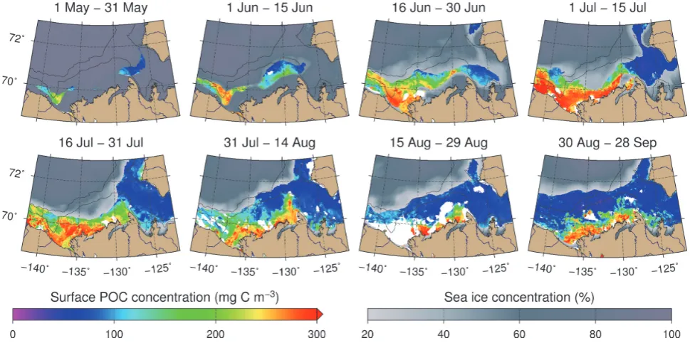
Fig. 3. MERIS composites of surface POC concentrations from May to September 2009 in the southeast Beaufort Sea as estimated with an empirical relationship established between in situ POC and the blue-to-green ratio of remote-sensing reflectance (490, 560 nm) measured during the CASES 2004 and Malina 2009 field campaigns. Sea ice concentration data (grayish scale, from 20 % to 100 % ice cover) as obtained from the SSM/I-DMSP orbiting sensor were superimposed over the satellite composites of surface POC concentrations (1 km resolution, 5 km radius interpolation). White patches correspond to ice-free areas within which no MERIS data were available during the time period due to the presence of clouds. The two bathymetric contour lines in each figure correspond to the 100 and 1000 m isobaths.

any spectacular increase in downward POC fluxes. When daily fluxes from all time series are cumulated and aver-aged for an annual cycle, the estimated mass flux across the Mackenzie Shelf region was higher at 200 than at 100 m depth (136 vs. 60 g DW m−2_yr−1_{). However, the} av-erage vertical POC flux was relatively similar at both depths (6.9 vs. 6.4 g C m−2yr−1). The C : N ratios of particulate or-ganic matter fluxes recorded with long-term traps generally oscillated between 6 and 10, with no clear seasonal or verti-cal pattern among time series (Fig. 6).

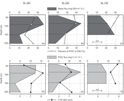
Vertical particle fluxes recorded with the short-term traps at three stations in the third week of August 2009 (Table 1) exhibited a similarly low magnitude ranging from ∼ 11– 54 mg DW m−2d−1 (Fig. 7), which was much lower than the average mass flux (∼ 270 mg DW m−2d−1) estimated for this period with the long-term traps. This was linked to the minuscule, but actual, quantity of particulate matter ob-served in the upper 200 m of drifting trap stations when sam-pling took place (see Figure A1). It should be noted, how-ever, that low mass fluxes (<50 mg DW m−2_d−1_{)were also} detected with the long-term traps at some stations or occa-sions in summer (Fig. 6), such as in previous studies of parti-cle fluxes in the Beaufort Sea and elsewhere (Table A1). The percentage of POC in vertical mass fluxes at drifting stations 345, 235, and 135 was relatively uniform (24±6 %). Hence, vertical patterns of POC fluxes in short-term traps (Fig. 7d–

f) followed those of mass fluxes. The C : N ratio of vertical fluxes recorded with short-term traps (6–9) was in the same range as the C : N ratio of fluxes collected with long-term traps (Figs. 6–7).

3.3 Vertical particle flux dynamics as obtained from the

UVP5 dataset

We obtained 21 overlaps between sediment trap sampling and UVP5 deployments over the course of the field cam-paign in July–August. The optimization procedure generated power-law parameters (Table 2) that transformed particles within the size range of 0.08–4.2 mm ESD into vertical mass and POC flux estimates with relatively strong coefficients of determination (r2=0.73 for DW fluxes;r2=0.68 for POC fluxes; Fig. 8). A multiple random resampling exercise of our database (Appendix A, Fig. A1b) enabled us to estimate a standard deviation corresponding to ∼20 % up to∼33 % of the variousAandbparameters (Table 2), which is in the range of comparable previous studies. The scaling exponent

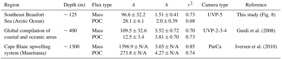
Table 2. Constant (A)and scaling exponent (b)of the empirical power-law relationships (±standard deviation) computed by the Nelder-Mead simplex minimization procedure between particle size determined by underwater cameras and the corresponding mass and particulate organic carbon (POC) fluxes measured with in situ sediment traps. The associated coefficients of determination (r2)describe the fits between the estimated fluxes using empirical equations and the sediment trap fluxes. See also Appendix A for a sensitivity analysis conducted on theAandbparameters. N/A: not available.

Region Depth (m) Flux type A b r2 Camera type Reference

Southeast Beaufort ∼125 Mass 96.6±32.2 1.51±0.41 0.73 UVP-5 This study (Fig. 8)

Sea (Arctic Ocean) POC 28.1±6.1 2.0±0.39 0.68

Global compilation of ∼400 Mass 109.5±32.6 3.52±0.72 0.70 UVP-2-3-4 Guidi et al. (2008) coastal and oceanic areas POC 12.5±3.4 3.81±0.70 0.73

Cape Blanc upwelling ∼1300 Mass 1396.9±N/A 3.65±N/A 0.85 ParCa Iversen et al. (2010) system (Mauritania) POC 273.8±N/A 4.27±N/A 0.74

When applied to the whole UVP5 dataset, vertical POC fluxes across the Mackenzie Shelf region can be conveniently plotted for a 3-D domain (Fig. 9). This enables quick grasp-ing of the main vertical flux structures, patterns and gradi-ents. For an in-depth description on how Fig. 9 was made and a further 3-D interactive visualization of POC fluxes across the study region using geographic information sys-tem (EnterVol for ArcGIS, C Tech, USA), see Appendix C and the online Supplement. The 7 Malina sections mapped in Fig. 1 are illustrated as 2-D cross-shelf vertical planes in Fig. 9, whereas ArcticNet stations located on the middle shelf and other Malina stations correspond to the small along-shelf planes. Vertical POC fluxes >75 mg C m−2_d−1 _were restricted to the shelf environment (<100 m isobath) and to the benthic boundary layer on the slope, in particular in Kug-mallit Valley and close to the Mackenzie Canyon (Fig. 9). At some locations on the inner shelf and in the Mackenzie Canyon, vertical POC fluxes, as estimated with our empir-ical relationships, were remarkably high – such as at shal-low stations 380/390 and 680/690 (Fig. 1), where POC fluxes ranged from∼1 up to∼5 g C m−2d−1. Relatively high POC fluxes (>75 mg C m−2d−1)were also detected at the begin-ning of the cruise in July when compared with the whole dataset, and especially with data obtained for the third week of August when fluxes were overall very low (e.g., line 400, stations 235 and 135; also short-term trap deployments as seen in Fig. 7). Around Cape Bathurst, part of the high POC fluxes on the shelf appeared to feed a lateral (i.e., oblique) ex-port of POC toward the deeper layers (Fig. 9). At the mouth of Amundsen Gulf, the abrupt transition from a high-to-low POC flux regime was linked to a real shift in the particle abundance from Cape Bathurst to Banks Island – and not to an artifact of the visualization software.

Cumulated histograms of average vertical fluxes for each size class along the size spectrum for the inshore and off-shore environments (delimited by the shelf break, 100 m iso-bath) illustrated that mass fluxes over the shelf were about 8 times higher than offshore and that POC fluxes were fivefold

greater (Fig. 10). Roughly 50 % of vertical mass fluxes were induced by particles less than 170 µ m (shelf) or 210 µ m (off-shore) (Fig. 10). In particular, a substantial fraction of mass fluxes (20 % inshore, 15 % offshore) was contained in the smallest size class of 80–100 µ m ESD (Fig. 10a, b). A sim-ilar trend was detected for mean vertical POC fluxes, within which half was comprised in the lower range of the size spec-trum for both the inshore (<260 µm) and offshore (<300 µm) environments. However, the contribution of smallest parti-cles was not that high for POC fluxes offshore, where the size class 260–330 µ m was actually the most important contrib-utor (12 %). Overall, ca. 77 % of both mass and POC fluxes were contained in size classes below 500 µm.

The modeled settling speed as a function of the coeffi-cientA and scaling exponentb (thus of the fractal dimen-sion) of the mass flux power-law equations (Table 2) were plotted for each size class along the particle size spectrum 0.08–4.2 mm ESD (Fig. 11). This revealed that particles in the lower size range (<300 µm) in the Mackenzie Shelf re-gion were apparently sinking faster (up to∼10 times) than in other studies, within which theAandbparameters were computed in a similar manner and for which a higher fractal dimension has been obtained (Fig. 11, Table 2). Conversely, the modeled (idealized) settling rate of particles larger than 1 mm. ESD (which represented a minor portion of the total fluxes; see above) was much lower in the southeast Beaufort Sea than in other systems. Based on our dataset, the max-imum “average” velocity of the population of sinking par-ticles was∼45 m d−1 for the largest size class centered on 3.8 mm ESD, which contributed to∼1 % of total mass fluxes (Fig. 10a, b).

3.4 Temporal variability of biotic and abiotic

components in the water column

4 0 25 50 75

1 0 2

Chl

a

fluorescence

(mg Chl

a

m

-3)

10

0.1

10

1 100

-0.8

-1.2 -0.4

-1.6

34

33

32

31

Turbidity (NTU)

Temperature

(°C)

Salinity

Sea ice concetration

(%)

PAR

(µmol quanta s

-1 m -2)

Jan Feb Mar Apr May Jun Jul Aug Sep Sea ice

concentration

(b)

(c)

(d)

(e)

(f)

PAR

Fluorescence

Turbidity

Temperature

Salinity

57 m 54 m

178 m

57 m 54 m

178 m

178 m

57 m

N/A 54 m 54 m

Fig. 4. Time series from January to September 2009 at mooring CA05 of (a) ice concentration (12.5×12.5 km pixel over the moor-ing); (b) photosynthetically active radiation at∼54 m; (c) chloro-phylla fluorescence at 54 m; (d) turbidity at 54, 57, and 178 m (measured with three different types of sensor; see Sect. 2.4 for de-tails); (e) temperature at 54, 57, and 178 m; and (f) salinity at 57 and 178 m. These variables aim at showing the general seasonality of the pelagic environment in southeast Beaufort Sea prior to the 2009 ArcticNet-Malina field campaign. N/A: no data available.

20 10 0 10 20 30

10

20 0 10

10

10 0 10

20 10 0

Current velocity (cm s

-1)

North

Jan Feb Mar Apr May Jun Jul Aug Sep

22 m

51 m

80 m

178 m (b)

(c)

(d)

Fig. 5. Time series from January to September 2009 of daily low-pass-filtered current vectors recorded at 22, 51, 80 and 178 m depth at mooring CA05. These current vectors aim at presenting the gen-eral seasonality of ocean circulation around the Mackenzie Shelf prior and during the 2009 ArcticNet-Malina field campaign. The location of the mooring is given in Fig. 1 and details of the deploy-ment in Table 1.

coefficient, zooplankton biomass, and bacterial production (BP) throughout the ArcticNet-Malina campaign (Fig. 12). These variables were available at the same spatial and tem-poral resolution than the POC fluxes, except for BP for which part of the time series was replaced by a statistical model (r2=0.71, n=339) based on temperature and carbon re-source (see Appendix D for details).

From 18 July to 23 August 2009, concentration of Chl

Vertical mass fluxes Percent of POC Vertical POC fluxes C:N ratios

S O N D

J F M A M J J A S O N D

2009

J F M A M J J A

2009 CA05 108 m CA16 110 m CA16 211 m A1 95 m A1 200 m G09 100 m G09 200 m

Mass flux (mg DW m

-2 d -1)1200

0 300 600 900

Percent of POC in DW (%)

40

0 10 20 30

POC flux (mg C m

-2 d -1)120

90

60

30

0

C:N ratio (a:a)

10.0

8.5

7.0

5.5

4.0

Mass flux (mg DW m

-2 d -1)1200

0 300 600 900

Percent of POC in DW (%)

40

0 10 20 30

POC flux (mg C m

-2 d -1)120

90

60

30

0

C:N ratio (a:a)

10.0

8.5

7.0

5.5

4.0

Mass flux (mg DW m

-2 d -1)1200

0 300 600 900

Percent of POC in DW (%)

40

0 10 20 30

POC flux (mg C m

-2 d -1)₁₂₀

90

60

30

0

C:N ratio (a:a)

10.0

8.5

7.0

5.5

4.0

Mass flux (mg DW m

-2 d -1)1200

0 300 600 900

Percent of POC in DW (%)

40

0 10 20 30

POC flux (mg C m

-2 d -1)120

90

60

30

0

C:N ratio (a:a)

10.0

8.5

7.0

5.5

4.0

Mass flux (mg DW m

-2 d -1)1200

0 300 600 900

Percent of POC in DW (%)

40

0 10 20 30

POC flux (mg C m

-2 d -1)₁₂₀

90

60

30

0

C:N ratio (a:a)

10.0

8.5

7.0

5.5

4.0

Mass flux (mg DW m

-2 d -1)1200

0 300 600 900

Percent of POC in DW (%)

40

0 10 20 30

POC flux (mg C m

-2 d -1)120

90

60

30

0

C:N ratio (a:a)

10.0

8.5

7.0

5.5

4.0

Mass flux (mg DW m

-2 d -1)1200

0 300 600 900

Percent of POC in DW (%)

40

0 10 20 30

POC flux (mg C m

-2 d -1)120

90

60

30

0

C:N ratio (a:a)

10.0 8.5 7.0 5.5 4.0 N/S N/S N/S N/S N/S N/S N/S N/S N/S N/S N/S N/S N/S N/S (a) (b) (c) (d) (e) (f) (g) (h) (i) (j) (k) (l) (m) (n)

30

30 45

20 10 0

15 0

50

150 100

200

Depth (m)

30

30 45

20 10 0

15 0

30

30 45

20 10 0

15 0

5

0 10 15

9 7

5 50

150 100

200

Depth (m)

5

0 10 15

9 7

5

5

0 10 15

9 7

5

Mass flux (mg DW m-2 _d-1₎

Percent of POC in DW (%)

POC flux (mg C m-2 _d-1₎

C:N ratio (a:a) (a)

N/S

N/S

(b) (c)

(d) (e) (f)

Fig. 7. Vertical profiles of daily vertical mass fluxes (dry weight, DW), percentage of POC in DW, particulate organic carbon fluxes (POC), and C : N ratios, recorded with short-term drifting traps deployed at stations 345 (a, d), 235 (b, e), and 135 (c, f), during the Malina 2009 campaign. The location of the short-term traps is given in Fig. 1 and details of the deployments in Table 1. N/S: no sampling.

upper slope of the Mackenzie Trough (124 m bottom depth). The beam attenuation coefficient followed a similar inshore-offshore gradient than Chla, but did not mirror the fluores-cence pattern at every station (Fig. 12). In particular, numer-ous features of increased beam attenuation coefficient did not have their equivalent in the Chlatime series.

Zooplankton biomass as evaluated with the UVP5 over the Mackenzie Shelf (inshore zone) was generally concen-trated in water layers underneath the Chlamaxima (Fig. 12). Highest biomass (bottom-surface) was found over the inner shelf (∼ 7 g C m−2) in late July (Fig. 13). Offshore, zoo-plankton biomass was markedly patchy, with an apparent vertical deepening of the biomass (Fig. 12) and declining trend (Fig. 13) over the first half of the sampling period. In both zones, zooplankton biomass was low (∼1 g C m−2) af-ter the first week of August. Overall, zooplankton biomass was overwhelmingly dominated by copepods (Fig. 13), but appendicularians accounted for an increased fraction of the biomass (∼15 %) over the shelf when copepod biomass was low in late August. The combination of measured and mod-eled BP over July–August reflected a close association with the beam attenuation coefficient pattern (Fig. 12). As in other

variables, BP was distinctively higher (>2 mg C m−3_d−1₎ over the shelf than in the offshore area, except in early Au-gust, when stations on the upper slope of the Mackenzie Trough were sampled (Fig. 12).

3.5 Spatial structures and variation partitioning of

POC flux forcing factors

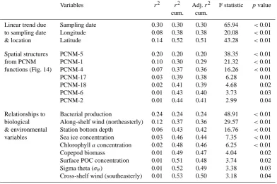
The first step toward the computation of the variation parti-tioning analysis was to calculate the linear trend due to sam-pling date and location, as well as to obtain all the significant spatial PCNM functions and physical–biological variables needed to perform the analysis. The linear trend between POC flux size classes and sampling date and location was significant (p<0.01). It could explain 52 % of the variability in the vertical flux data, with date as the main factor (Ta-ble 3). Redundancy analysis (RDA) and associated triplot of the linear trend model (Fig. 14a) illustrated that POC fluxes were negatively correlated with sampling date. The mean co-sine of the angle between the date vector and POC flux size classes (≈correlation) was−0.92±0.05.

Table 3. Output from the forward selection of explanatory variables of vertical POC fluxes (154 stations, 17 size classes each, all integrated over the top 200 m of the water column) based on the double criterion procedure as described in Borcard et al. (2011). For parsimony purpose, only the resulting reduced models of significant variables (p≤0.05) were used in the redundancy analyses (Fig. 14) and in the variation partitioning analysis of POC fluxes (Fig. 16). The list of all biophysical variables available for the present study is presented in Table 4. PCNM: principal coordinates of neighbor matrices (Borcard et al., 2011).

Variables r2 r2 Adj.r2 F statistic pvalue cum. cum.

Linear trend due Sampling date 0.30 0.30 0.30 65.94 <0.01 to sampling date Longitude 0.08 0.38 0.38 20.08 <0.01

& location Latitude 0.14 0.52 0.51 43.28 <0.01

Spatial structures PCNM-5 0.20 0.20 0.20 38.35 <0.01

from PCNM PCNM-1 0.10 0.30 0.29 21.32 <0.01

functions (Fig. 14) PCNM-4 0.07 0.37 0.36 16.26 <0.01

PCNM-17 0.03 0.39 0.38 6.28 0.01

PCNM-18 0.02 0.41 0.39 4.68 0.02

PCNM-6 0.01 0.43 0.40 3.73 0.03

PCNM-2 0.01 0.44 0.41 2.99 0.04

Relationships to Bacterial production 0.24 0.24 0.24 48.91 <0.01 biological Along-shelf wind (northeasterly) 0.12 0.37 0.36 29.57 <0.01 & environmental Station bottom depth 0.06 0.43 0.42 16.76 <0.01 variables Sea ice concentration 0.03 0.46 0.44 7.35 <0.01 Chlorophyllaconcentration 0.02 0.48 0.46 6.25 <0.01

Copepod biomass 0.01 0.49 0.47 4.04 0.02

Surface POC concentration 0.01 0.51 0.48 3.74 0.02

Sigma theta (σθ) 0.01 0.52 0.49 3.38 0.03

Cross-shelf wind (southeasterly) 0.01 0.53 0.50 3.18 0.04

integrated for the upper 200 m of the water column produced a series of 25 PCNM with positive Moran’s I. The truncation threshold distance resulting from the spanning tree among station sites was 77.9 km. The forward selection retained 7 significant PCNM variables (Fig. 15a–g) that explained 44 % of the undetrended POC flux data (Table 3). The PCNM-5 (Fig. 15d) was the most important structure (r2=0.20, Ta-ble 3) and was strongly correlated with POC fluxes as ob-served through the RDA triplot (Fig. 14b; mean cosine of the angle between POC fluxes and PCNM-5 was 0.97±0.02). The RDA between POC flux size classes, stations and PCNM variables generated three significant conical axes (p<0.05), but we retained only the first two in the triplot to ease the understanding of relationships in the multidimensional do-main (Fig. 14b). The third significant canonical axis was ex-plaining less than 1 % of the total PCNM variance. Maps of the fitted scores from the first two axes illustrated the main spatial structures of POC fluxes across the sampling region (Fig. 15h–i). The first axis can be seen as combination of PCNM-4, -5, and -17, whereas the second axis was related to PCNM-1, -2, -6, and 18 (Fig. 15). Multiple regressions between the fitted scores from the first two canonical axes of PCNM variance against the environmental variables avail-able in the present study provided insights on the physical–

biological determinants responsible of the orthogonal spatial structures (Table 4).

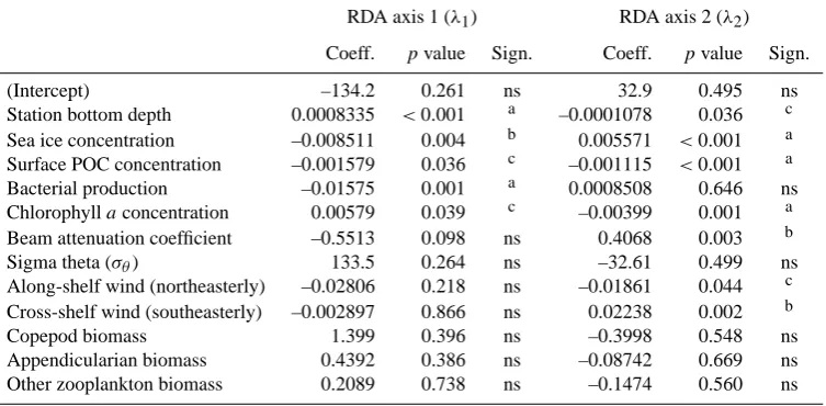
The RDA between POC fluxes and physical–biological variables produced a significant relationship (p<0.01) that was reduced to a parsimonious model of 9 significant param-eters (Table 3). The reduced model generated through for-ward selection explained 53 % of the POC flux data. Triplot of the reduced model (Fig. 14c) illustrated that BP and the northeasterly wind component were the two most important positive determinants. In particular, BP was closely related to small particles (0.08–0.42 mm, cosine=0.99±0.01), while northeasterly wind was associated with large aggregates (1.67–4.22 mm, cosine=0.94±0.04). Interestingly, the av-erage water density in the upper water column (σθ, 0–50 m)

had also a strong correlation with POC fluxes (mean cosine

=0.98±0.01). The two variables with the most negative cor-relations were bottom depth (mean cosine= −0.88±0.06) and copepod biomass (mean cosine= −0.84±0.07).

44.5 % and 5.0 % of the total PCNM variance, Fig. 15h–i) against the set of environmental and biological variables available in the present study. PCNM: principal coordinates of neighbor matrices (Borcard et al., 2011).

RDA axis 1 (λ1) RDA axis 2 (λ2)

Coeff. pvalue Sign. Coeff. pvalue Sign.

(Intercept) –134.2 0.261 ns 32.9 0.495 ns

Station bottom depth 0.0008335 <0.001 a –0.0001078 0.036 c Sea ice concentration –0.008511 0.004 b 0.005571 <0.001 a Surface POC concentration –0.001579 0.036 c –0.001115 <0.001 a Bacterial production –0.01575 0.001 a 0.0008508 0.646 ns Chlorophyllaconcentration 0.00579 0.039 c –0.00399 0.001 a Beam attenuation coefficient –0.5513 0.098 ns 0.4068 0.003 b

Sigma theta (σθ) 133.5 0.264 ns –32.61 0.499 ns

Along-shelf wind (northeasterly) –0.02806 0.218 ns –0.01861 0.044 c Cross-shelf wind (southeasterly) –0.002897 0.866 ns 0.02238 0.002 b

Copepod biomass 1.399 0.396 ns –0.3998 0.548 ns

Appendicularian biomass 0.4392 0.386 ns –0.08742 0.669 ns Other zooplankton biomass 0.2089 0.738 ns –0.1474 0.560 ns

Significance:a_:p≤0.001,b_:p≤0.01,c_{:p≤0.05, ns: nonsignificantp >0.05.}

due to sampling date, Table 3) and the two other models were also detected. The pure linear and PCNM spatial trends were relatively low (4.2 % and 6.7 %), whereas the pure trend due to biotic and abiotic variables was 13.0 %. The nega-tive percentage between the PCNM and environmental mod-els (−1.5 %) indicates that the contributions from these two submodels when taken separately are larger than their partial contributions.

4 Discussion

4.1 Seasonal variability of the atmosphere–ice–ocean

interface and vertical particle fluxes in Beaufort Sea during 2009

Mean ice concentration over the Mackenzie Shelf in 2009 was near the average of years 1998-2008, but the high stan-dard deviation (∼ 25 %) associated with the mean sea ice from June to August reflected the strong interannual variabil-ity of ice conditions in the Beaufort Sea in summer (e.g., Gal-ley et al., 2008). In fact, ice conditions were heavier in 2009 than during the previous 5 years, when intensive sampling was conducted in the region as part of the CASES, Arctic-Net and CFL programs, but were less severe in 2009 than over the period of 2000–2003, when the mean ice concen-tration remained above 40 % until August (CIS, 2009). Part of the reason why sea ice was relatively heavy in summer 2009 was linked to the persistent northerly winds of June– July (Fig. 2a) that induced the southward advection of large sea ice floes from the central Arctic pack. During that time a

high-pressure system was located over the northern Beaufort Sea (NSIDC, 2009). But as soon as the atmospheric pres-sure declined in late July, the northerly wind pattern relaxed and broke up, thus generating wind conditions over August that were more variable and generally from the south. This shift in the atmospheric pressure brought also cloudy condi-tions as well as divergence (i.e., spreading and melt) of the remaining sea ice cover. Hence, a substantial fraction (up to

∼60 %) of the surface layer (<10 m) across the study re-gion was comprised of sea ice melt water in August 2009, with an increasing proportion from the ice-free shelf toward the partly ice-covered basin (Lansard et al., 2013). Another source of freshwater was the Mackenzie River, which dis-charged 13 % more water during 2009 when compared with the average annual value of years 1998–2008 (Fig. 2c) – even if the runoff in August appears to have been lower than the mean. As a result, the upper water column during our field campaign was highly stratified and nitrate (the limiting nu-trient in Beaufort Sea) was depleted in the top 40 m, except near the river delta and on the eastern shelf, north of Cape Bathurst (Raimbault et al., 2011). Unfortunately, we do not know the history of nutrient fields in the area prior to late July and we have to rely on moorings and satellite imagery to infer spring/early summer productivity.

10 100 1000

10 100

10 100 10 100 1000

Sediment trap mass flux (mg DW m-2 _d-1₎

Sediment trap POC flux (mg C m-2 _d-1₎

UVP-derived mass flux (mg DW m

-2 d -1)

UVP-derived POC flux (mg C m

-2 d -1) (a)

(b)

Slope = 0.68 ± 0.09 Intercept = 23.39 ± 2.53

r2 _{= 0.73}

p < 0.01

n = 21

Slope = 0.74 ± 0.11 Intercept = 4.56 ± 2.01

r2 _{= 0.68}

p < 0.01

n = 21

Fig. 8. Regressions of vertical mass fluxes (a) and particulate or-ganic carbon (POC) fluxes as estimated with the UVP5 dataset and the empirical equations obtained with the minimization procedure (Table 2) against the mass fluxes and POC fluxes recorded by the in situ sediment traps (Table 1). See Appendix A for a rationale and sensitivity analysis conducted on the empirical equations obtained with the optimization technique.

the Alaskan shelf under the effect of persistent northerlies. As landfast ice broke up, the increase of surface POC con-centration nearshore was probably linked as well to au-tochthonous primary production. However, it is difficult to conclude on the exact contribution of each carbon source to the surface POC pool as based solely on satellite images. Cloudy conditions hindered the collection of sufficient satel-lite images to produce complete composites in August, but data collected in situ during the Malina campaign showed that the maximum turbidity zone of the Mackenzie River was restricted to waters within the 10 m isobath (Doxaran et al., 2012). The particulate backscattering ratio measured

nearshore revealed that particulate matter in this area was mineral rich (i.e., around 2–4 % POC). Between the 10 and 50 m isobath, a transition zone characterized by the near-surface (<4 m) spreading of the river plume overlying a rel-atively clear water column was observed. Beyond the 50 m depth boundary, the concentration of riverine material was low and the water optical properties were indicative of a sys-tem driven by phytoplankton-derived particles (Doxaran et al., 2012). These findings confirm that sediments carried by the Mackenzie River plume sink quasi-exclusively nearshore (cf. O’Brien et al., 2006) despite that riverine freshwater and dissolved organic matter may be transported beyond the shelf break (Matsuoka et al., 2012; Lansard et al., 2013). In fact, an exhaustive suite of molecular biomarker assays conducted on particles sampled at the shelf periphery in August indi-cated that particles beyond the shelf break were of marine origin at ∼99 % (Tolosa et al., 2013). Therefore, the ma-terial collected by sediment traps was obviously originating from a marine source, at least during the spring–summer pe-riod, when it is known to be the case in the area (Sampei et al., 2011 and references therein). Lipid tracer analyses of sediment trap samples collected at CA05, CA16, and G09 (Fig. 1) in July–August confirmed that sinking material was derived from planktonic productivity (Rontani et al., 2012).

Interestingly, the peak vertical POC flux over the 2009 an-nual cycle occurred in August, at the same time as Chla flu-orescence appeared to have reached its maximum at∼50 m depth (Fig. 4). This synchronicity supports our previous de-duction that vertical POC fluxes resulted primarily from local biological activity. According to previous studies that docu-mented the evolution of Chla over the spring–summer pe-riod in Beaufort Sea (e.g., Tremblay et al., 2008; Forest et al., 2011), the rise in fluorescence detected at∼50 m depth at CA05 was the continuum of the spring bloom that typi-cally lowers the nutricline as the summer season progresses. This subsurface chlorophyll maximum (SCM) was also well defined in the Chl a time series in both inshore and off-shore zones (Fig. 12), corroborating its widespread nature in the western Canadian Arctic (Martin et al., 2010). How-ever, POC fluxes recorded at long-term moorings remained relatively low in spring–early summer (<30 mg C m−2d−1)

Fig. 9. Three-dimensional view of vertical POC fluxes across the Mackenzie Shelf region as estimated with the empirical power-law equations from the minimization procedure (Table 2) and applied to the whole UVP5 dataset from the ArcticNet-Malina 2009 campaign. Each vertical section corresponds to a specific transect as shown in Fig. 1. A MERIS composite of surface POC concentrations encompassing the period from 18 July–23 August 2009 is superimposed above the vertical POC fluxes. For convenience, we show only the vertical POC fluxes since the mass flux pattern is analogue to POC when using the UVP5 dataset – i.e., the percentage of POC in dry-weight fluxes averaged 18.7 %±0.2 % (within 95 % confidence bounds,r2=0.95). See also Appendix C and the online Supplement for an interactive visualization of vertical POC fluxes across the study region using geographic information system (EnterVol for ArcGIS, C Tech, USA).

North Atlantic spring bloom). Hence, our results support that the patchiness of vertical POC fluxes should be considered when characterizing the biogeochemical status of a given re-gion on the basis of a few vertical flux measurements.

The seasonal pattern provided by long-term trap records (Fig. 6) suggests two nonexclusive possibilities: (1) that the magnitude of the spring bloom in 2009 was lower than usual or (2) that most of the primary production in spring–early summer was intercepted by grazers and retained within the pelagic food web. Of course, the dynamics of the spring bloom in 2009 is not actually known, even if we can assume that phytoplankton production was the main driver of the in-creased POC signal associated with the receding ice cover as seen on MERIS images in May–June (Fig. 3). In the Arc-tic Ocean, zooplankton grazers are usually primed to feed on the wealth of high-quality food available as soon as the spring bloom starts (see Forest et al., 2011 and references therein). Hence, the sinking POC in mid-to-late summer can be viewed as what heterotrophic plankton were not able to assimilate from the decaying bloom/SCM, whatever was its magnitude. Average export at∼100 m depth for the month of August 2009 at the shelf margin was ca. 2 g C m−2. This cu-mulated value corresponds to a sampling covering less than 10 % of a year cycle, but accounts for roughly half of the average annual autochthonous export (∼4 g C m−2)usually

recorded with 100 m sediment traps in the region from 2003-2008 (Forest et al., 2010a; Sampei et al., 2011; Forest et al., 2011). Hence, the Malina campaign should be seen as the time window representing optimal conditions for studying processes regulating vertical export at a fine spatial scale. This is particularly true as current velocities recorded during that period were generally low (∼4–10 cm s−1), which is a good indicator that particle fluxes recorded with our Techn-icap sediment traps were not biased by any strong hydrody-namic flow (e.g., Forest et al., 2010a; Sampei et al, 2011), and thus could be used in further analysis – such as toward the development of an algorithm linking sediment trap data to the particle size distribution recorded by an underwater camera.

4.2 Particle fractal properties and spatial patterns of

vertical POC fluxes in mid-summer 2009 across the Mackenzie Shelf

100 80 60 40 20 0 100 80 60 40 20 0 100 80 60 40 20 0 100 80 60 40 20 0 330 270 210 150 90 30 44 36 28 20 12 4 27.5 22.5 17.5 12.5 7.5 2.5 5.5 4.5 3.5 2.5 1.5 0.5

Cumulated mass flux (%)

Cumulated mass flux (%)

Cumulated POC flux (%)

Cumulated POC flux (%)

V

e

rtical mass flux (mg DW m

2 d -1)

V

e

rtical mass flux (mg DW m

2 d -1)

V

e

rtical POC flux (mg C m

2 d -1)

V

e

rtical POC flux (mg C m

2 d -1)

0.08 - 0.100.10 - 0.1

3

0.13 - 0.170.17 - 0.2

1

0.21 - 0.260.26 - 0.330.33 - 0.4

2

0.42 - 0.530.53 - 0.6

6

0.66 - 0.8 4

0.84 - 1.0 5

1.05 - 1.3 3

1.33 - 1.6 7

1.67 - 2.1

1

2.11 - 2

.66

2.66 - 3.3 5

3.35 - 4.22 0.08 - 0.1

0

0.10 - 0.130.13 - 0.170.17 - 0.210.21 - 0.2

6

0.26 - 0.3 3

0.33 - 0.420.42 - 0.5

3

0.53 - 0.660.66 - 0.840.84 - 1.051.05 - 1.3

3

1.33 - 1.671.67 - 2.1

1

2.11 - 2.

66

2.66 - 3.353.35 - 4.22

Vertical mass fluxes Cumulated fluxes Vertical POC fluxes Cumulated fluxes

(a)

(b) (d)

(c)

Size-class ESD (mm) Size-class ESD (mm)

Offshore Inshore

Offshore Inshore

Fig. 10. Histograms of average vertical mass fluxes (a, b) and vertical POC fluxes (c, d) within each size class considered to estimate the fluxes using the empirical equations and the UVP5 dataset. The relative cumulated flux for each size distribution is also presented in each panel. Absolute cumulated fluxes (total of all size classes) in the inshore and offshore zone were (a, b) 1646 and 263 mg DW, m−2d−1for the mass fluxes, respectively, whereas they were (c, d) 244 and 43 mg C m−2d−1for the POC fluxes, respectively. The inshore and offshore regions are delimited by the 100 m isobath, which corresponds to the shelf break. Vertical bars depict the standard error associated with each vertical flux size class.

to estimate vertical fluxes with the particle size distribution recorded with a UVP5. The resulting empirical equations were, however, different from the ones obtained previously in various low-latitude marine ecosystems (Table 2). In par-ticular, the scaling exponent b (and thus the mean fractal dimension D)of vertical mass fluxes in Beaufort Sea was more than twice lower than the values calculated by Guidi et al. (2008) and Iversen et al. (2010). Actually, the fractal dimension (1.26±0.34) of mass fluxes estimated here was in the lowest range of what is typically observed through-out diverse marine aggregates (i.e., from 1.1 to 2.3; Guidi et al., 2008 and references therein). According to fractal geom-etry theory, such low fractal dimensionDimplies that sink-ing particles were apparently more porous, fluffy and/or fil-amentous than in other marine ecosystems (e.g., Logan and Wilkinson, 1990; Logan and Kilps, 1995; Guidi et al., 2008). Here, the main reason why the fractal dimension was low is likely linked to our sediment trap sampling design that was centered around 125 m, whereas previous studies used trap measurements from∼400 to∼1300 m depth (Table 2). This comparison supports the view that settling particles get more compact as they sink because of various processes such as coagulation, grazing, and microbial degradation (Guidi

et al., 2008; Burd and Jackson, 2009). Our mathematical analyses thus suggest that sinking material in the epipelagic layer of our study region in July–August 2009 was primar-ily composed of “fresh” marine debris (e.g., phytodetritus, fecal pellets, exudates) recently agglomerated within a fluffy and sticky gel-like matrix that would induce an overall fractal dimension around∼1.3 (e.g., Logan and Wilkinson, 1990). This also corroborates the results of Rontani et al. (2012) and Tolosa et al. (2013), who found a strong marine signature in suspended and sinking matter in the upper water column of the Beaufort Sea during the Malina campaign.