Measurement depth effects on the apparent temperature sensitivity of soil respiration in field studies

© Author(s) 2008. This work is distributed under the Creative Commons Attribution 3.0 License.

Measurement depth effects on the apparent temperature sensitivity

of soil respiration in field studies

A. Graf, L. Weiherm ¨uller, J. A. Huisman, M. Herbst, J. Bauer, and H. Vereecken

Forschungszentrum J¨ulich, Agrosphere Institute (ICG-4), Institute for Chemistry and Dynamics of the Geosphere, 52425 J¨ulich, Germany

Received: 7 April 2008 – Published in Biogeosciences Discuss.: 6 May 2008 Revised: 18 July 2008 – Accepted: 29 July 2008 – Published: 26 August 2008

Abstract. CO2efflux at the soil surface is the result of

respi-ration in different depths that are subjected to variable tem-peratures at the same time. Therefore, the temperature mea-surement depth affects the apparent temperature sensitivity of field-measured soil respiration. We summarize existing literature evidence on the importance of this effect, and de-scribe a simple model to understand and estimate the mag-nitude of this potential error source for heterotrophic res-piration. The model is tested against field measurements. We discuss the influence of climate (annual and daily tem-perature amplitude), soil properties (vertical distribution of CO2sources, thermal and gas diffusivity), and measurement

schedule (frequency, study duration, and time averaging). Q10 as a commonly used parameter describing the

temper-ature sensitivity of soil respiration is taken as an example and computed for different combinations of the above con-ditions. We define conditions and data acquisition and anal-ysis strategies that lead to lower errors in field-basedQ10

determination. It was found that commonly used tempera-ture measurement depths are likely to result in an underesti-mation of temperature sensitivity in field experiments. Our results also apply to activation energy as an alternative tem-perature sensitivity parameter.

1 Introduction

Soil respiration is increasingly recognized as a major factor in the global carbon cycle. Due to a rising interest in the feedback between soils and climate change, numerous stud-ies have provided relations between temperature and soil res-piration either obtained in the laboratory or in the field.

Typ-Correspondence to: A. Graf

([email protected])

ically, the temperature sensitivity of soil respiration is ex-pressed as theQ10value, i.e. the factor by which respiration

is enhanced at a temperature rise of 10 K (Appendix A). Several restrictions to the significance of theQ10concept,

especially if mistaken as a means to extrapolate soil CO2

losses into a warmer future, have been brought up (David-son and Janssens, 2006; Tuomi et al., 2008). Here, we exam-ine an additional restriction which has received remarkably little attention in literature. In most field studies, column-integrated soil respiration and its sensitivity are quantified by a single temperature measurement, while the total flux is a sum of source terms from various depths, which are ex-posed to different temperature regimes. Because of the at-tenuation and phase shift of temperature fluctuations with in-creasing depth, the apparentQ10will depend on the

temper-ature measurement depth. This possibility was mentioned first by Lloyd and Taylor (1994), but without quantification. Davidson et al. (1998) predicted thatQ10 values would

in-crease with temperature measurement depth, and recognized that this complicates comparisons between studies. Recently, several field studies with multiple temperature measurement depths have been published (Xu and Qi, 2001; Hirano et al., 2003; Tang et al., 2003; Gaumont-Guay et al., 2006; Khomik et al., 2006; Shi et al., 2006; Wang et al., 2006; Pavelka et al., 2007). All of them show an increase of apparentQ10 with

depth. The same effect has also been identified in model simulations by Hashimoto et al. (2006), and demonstrated exemplary with synthetical data in a recent overview paper by Reichstein and Beer (2008). In a laboratory incubation, Reichstein et al. (2005a) found strongly differing tempera-ture time series between two probe locations within the soil core, and used a multiple regession to consider both locations as sources.

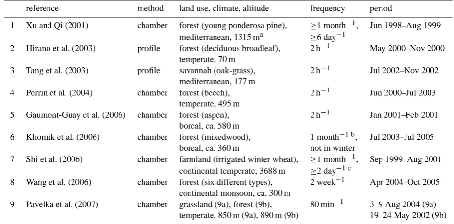
Table 1. Studies providing multipleQ10values due to multiple temperature measurement depths. Numbers refer to Fig. 2.

reference method land use, climate, altitude frequency period

1 Xu and Qi (2001) chamber forest (young ponderosa pine), ≥1 month−1, Jun 1998–Aug 1999 mediterranean, 1315 ma ≥6 day−1

2 Hirano et al. (2003) profile forest (deciduous broadleaf), 2 h−1 May 2000–Nov 2000 temperate, 70 m

3 Tang et al. (2003) profile savannah (oak-grass), 2 h−1 Jul 2002–Nov 2002

mediterranean, 177 m

4 Perrin et al. (2004) chamber forest (beech), 2 h−1 Jun 2000–Jul 2003

temperate, 495 m

5 Gaumont-Guay et al. (2006) chamber forest (aspen), 2 h−1 Jan 2001–Feb 2001

boreal, ca. 580 m

6 Khomik et al. (2006) chamber forest (mixedwood), 1 month−1 b, Jul 2003–Jul 2005

boreal, ca. 360 m not in winter

7 Shi et al. (2006) chamber farmland (irrigated winter wheat), ≥1 month−1, Sep 1999–Aug 2001 continental temperate, 3688 m ≥2 day−1 c

8 Wang et al. (2006) chamber forest (six different types), 2 week−1 Apr 2004–Oct 2005 continental monsoon, ca. 300 m

9 Pavelka et al. (2007) chamber grassland (9a), forest (9b), 80 min−1 3–9 Aug 2004 (9a) temperate, 850 m (9a), 890 m (9b) 19–24 May 2002 (9b)

a_{results given separately for two sites}

b_{morning and afternoon of the measurement day in summer, once per day in transition months}

c_{on two days per month in summer, 8 times at some days}

most appropriate when temperature measurements at mul-tiple depths are available. Tang et al. (2003), Perrin et al. (2004) and Shi et al. (2006) use the temperature measurement depth yielding the highestR2. Gaumont-Guay et al. (2006) suggest that the temperature-efflux curve with the lowest hys-teresis indicates the most appropriate temperature measure-ment depth. Pavelka et al. (2007) also use the maximumR2 method, but additionally performed a crosscorrelation anal-ysis to align each depths temperature time series with the efflux. Since most studies use a single, more or less arbi-trary, temperature measurement depth, the effect of varying temperature measurement depth is often not considered.

The aim of this study is to quantify the error inQ10

de-termination caused by different temperature measurement depths as a function of soil properties, climate, and measure-ment schedule. To this end, we present a simple model and validate it against field measurements of heterotrophic res-piration. We consider this model as a tool that helps with the design of field studies with meaningful temperature mea-surement depths, and with a more appropriate interpretation of existing datasets.

2 Methods

2.1 Literature review

We found nine studies where multiple temperature measure-ment depths were used to derive apparentQ10depth profiles.

An overview about the flux methods, site characteristics, and time schedules is given in Table 1.

Two of these studies use continuous CO2 concentration

profile measurements in the soil to calculate half-hourly sur-face CO2effluxes validated against chamber measurements.

All other studies directly use a closed chamber system to measure CO2 efflux. Many studies use a nested approach

with one or more measurement days each month, and two to ten measurements per such day (Table 1). Some studies cover a period of less than a year, whilst others leave out the winter months for operational reasons.

We also obtainedQ10 values from studies with a single,

reported temperature measurement depth (Kim and Verma, 1992; Dugas, 1993; Davidson et al., 1998; Fang et al., 1998; Chen et al., 2002; Law et al., 2002; Borken et al., 2003; Lou et al., 2003; Savage and Davidson, 2003; Yuste et al., 2003; Novick et al., 2004; Takahashi et al., 2004; deForest et al., 2006; Humphreys et al., 2006; Moyano et al., 2008; Tang et al., 2008). Here, either chamber or micrometeoro-logical systems were used to measure soil CO2 efflux. In

Phase shifts t i , Amplitudes A i z i = 1 i = 2 ... 0 1 cm 2 cm ... 50 cm

[ ]

Efflux (t)

t 1 t 2 ...

[ ]

Eq. B3 (stepwise) Eq. B3

Temperature T( z , t ) z t 1 t 2 ... 0 1 cm 2 cm ... 50 cm

[ ]

Respiration S R ( T)

z t 1 t 2 ... 0 1 cm 2 cm ... 50 cm

[ ]

Eq. A1 or A2

Soil properties depth z thermal diffusivity D T temperature sensitivity Q 1 0 or E a source strength S R T r e f eff. CO2 diffusivity D

C O 2 /θ 0 1 cm 2 cm ... 50 cm variant input Eq.C2 (sub-timesteps)

CO₂diffusion?

∑

SR F T

Concentration c

( z , t) z t 1 t 2 ... 0 1 cm 2 cm ... 50 cm

[ ]

(Eq. A1 or A2)-1

. Study schedule Start: variant input Time step: here, 1h length: variant input

Annual Average Temperature

T

a vg: variant input Temperature climate characterization

i period length τ i phase shift &t i Amplitude A i

at z r e

f

1 1 yr 260 d variant input 2 1 d 15 h variant input 3 0.5 d 1 h variant input 4... other not used in this study

Depth of known amplitudes: zref

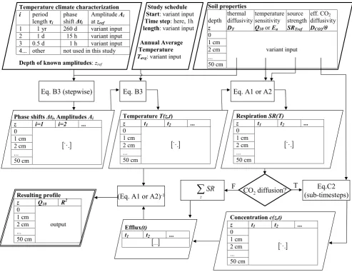
Fig. 1. Overview of the model architecture. Bold outline: Input parameters; doubled outline: Final output. Symbols are explained in the Appendix.

It should be noted that most studies addressed total soil res-piration, without differentiation between heterotrophic and autotrophic respiration.

2.2 Model

The model is based on the concept of thermal diffusion and is implemented in Fortran95. An overview of the model ar-chitecture is given in Fig. 1 and the theory behind the model is described in the Appendix. In brief, a simplified infinite near-surface temperature time series is generated using sev-eral distinct sine waves. The annual and diurnal cycle have a phase shift to correctly reproduce times of maxima and min-ima, assuming thatt=0 is new year’s midnight. A further cycle with a period of 12 h, a phase shift of 1 h, and an am-plitudeA=Adiurnal/4 was used to mimic the skewness of the

daily temperature cycle due to slow cooling during the night.

Variations of the diurnal amplitude and day length were not considered. The average temperature was set to the global average (15◦_{C) in the numerical experiments, and equalled}

the average measured temperature (12.7◦_{C) in the model}

val-idation. Input amplitudes are determined for the uppermost temperature sensor (0.5 cm) in the model validation. In the numerical experiments, amplitudes were provided for a ref-erence depth of 5 cm. The reason is that amplitudes in this depth are more similar to air temperature than the soil sur-face temperature. Air temperature amplitudes are globally available and provide a more common reference than surface temperature.

time averaged effect of soil moisture at each depth. On the other hand, time average effective thermal diffusivity may vary strongly with depth due to differences in soil properties and water content. To account for this, the analytic solution was applied in discrete depth steps of 1 cm, using the am-plitudes and phase shifts in each layer to calculate those of the next deeper layer (Appendix B). The model is run with a time step of 1 h. Soil respiration is calculated from tempera-ture using theQ10concept and, as an alternative, also using

the Arrhenius concept (see Appendix A). The source strength of respiration at the average temperature is also given as a depth-dependent value. Here, only a relative vertical distri-bution is required because absolute values have no effect on the resulting apparentQ10profile.

If CO2 diffusion time from each depth to the soil

sur-face is assumed to be insignificant, the efflux can simply be calculated by integration of the respiration over all depths. However, in analogy to the impact of thermal diffusion on the apparentQ10 discussed above, slow gas diffusion could

also affect the apparent Q10. To test this hypothesis, we

also included CO2 diffusion in several model runs. As

al-ready proposed for heat diffusion, we use an effective dif-fusivityDCO2θ

−1

a (Appendix C) invariant in time but verti-cally distributed. Because the concentration profiles are a result of the vertical source distribution and the nonlinear temperature dependence, CO2diffusion cannot be solved

an-alytically. Therefore, we implemented a numerical solution (Appendix C). The CO2 flux between two adjacent layers

is now the product of diffusivity and the concentration gra-dient. We assume no vertical exchange between the lowest layer and the underground. At the surface, a constant atmo-spheric CO2concentration of 16.5×103µmol m−3is

main-tained. The model considering diffusion requires initializa-tion of the concentrainitializa-tion profile. Therefore, the model uses a spin-up period. The length of the spin-up period is consid-ered adequate when the difference in cumulative efflux be-tween runs with and without diffusion is less than 1%.

Finally, the modelled time series of efflux at the surface and temperature in each depth are used to simulate the cur-rent practice of field-based Q10 determination. For each

depth, regression of log-transformed efflux against temper-atureT is used to computeQ10. To also test fitting of the

Arrhenius relation, the inverse of the temperature is plotted against log-transformed respiration. In this case, the result-ing activation energy is converted into aQ10 at the study’s

average temperature for comparison (cf. Sanderman et al., 2003).

2.3 Field measurements

An automated soil CO2flux chamber system (8100,

Li-Cor Inc., Lincoln, Nebraska, USA) was operated with four type T thermocouple thermometers at the FLOWatch project test site Selhausen of the Forschungszentrum J¨ulich. The test site is located in the river Rur catchment (50◦5200900N,

06◦₂₇0₀₁00_{E, 104.5 m above sea level). The climate is warm}

temperate, the soil is an Orthic Luvisol and the texture is silt loam according to the USDA classification. A detailed description of the test site is given by Weiherm¨uller et al. (2007). Organic carbon content was determined in vertical steps of 15 cm. In September 2006, the soil was tilled up to a depth of 15 cm and power harrowed. Bare field con-ditions were maintained by a repetition of this treatment in April 2007, several applications of glyphosate, and manual weed control at the efflux measurement plot. Historically, the field was annually ploughed to a depth of 30 cm, and the crop rotation was sugar beet – winter wheat. From 15 October 2006 to 24 April 2007 only one CO2 flux system

was used (closing interval every 30 min). From 24 April to 14 October 2007, four identical chambers with a separation of 20 cm were operated with the Li8100 multiplexer system (closing interval 15 min for each chamber). The soil flux chambers were placed on soil collars of 20 cm in diameter and a height of 7 cm, which were inserted 5 cm into the soil. The system was closed for two minutes for each flux mea-surement. CO2 and water vapour concentration as well as

chamber headspace temperature were measured every sec-ond, and the CO2 concentration was corrected for changes

in air density and water vapour dilution. The soil respiration was calculated by fitting a linear regression to the corrected CO2concentrations from 30 s after closing until reopening.

The thermocouples used to measure soil temperature have 1 mm thick unshielded joints to ensure a quick response, and were installed horizontally at 0.5, 3, 5, and 10 cm depth, 20 cm away from the chamber system. Temperature data were logged every second while the chamber was closed, and averaged. To vertically extend the empirical apparent Q10

profiles, we also use temperature data of pF-meters (Ecotech, Bonn, Germany) in 15, 30, 45, 60, 90 and 120 cm depth, which were logged independently in 1 h intervals.

To obtain a uniform dataset, the efflux and temperature measurements were reduced to median hourly CO2flux and

average hourly soil temperature at each measurement depth. In the case of CO2 flux, the median was used because it is

less sensitive to outliers and non-normal distributions. In the final data set, only those hours were considered where all flux and temperature measurements were available. Because more than 50% of the hours in December and January could not be considered due to power supply problems, these two months were completely excluded from the dataset.

1

8

7

1

3 2

6 5

4

9a

9b

-50 -40 -30 -20 -10 0

0 1 2 3 4 5 6 7 8 9 10 11 12

Q10

z

(

c

m

)

single depth study

multiple depth study

own measurements and model fit

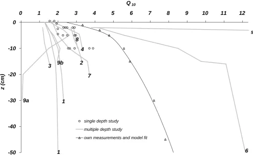
Fig. 2. Empirical apparentQ10as a function of temperature measurement depthz. Numbers refer to the study bibliography given in Table 1, single depth references are listed in the methods section. Depths>0 denote air temperature (height not to scale).

3 Results

3.1 Literature and own field measurements

Figure 2 shows apparentQ10 values as a function of depth

from this and other studies. An increase of apparentQ10

with depth can be seen in all studies, but with a strongly vari-able slope. The highest apparent value (Gaumont-Guay et al., 2006,Q10=150 in a temperature measurement depth of

50 cm) is not shown for scaling reasons. This profile is based on measurements taken during two winter months. The sec-ond highest value was found by Khomik et al. (2006), also at 50 cm, in long-term measurements excluding winter months, but including snow cover situations in spring, and capturing the diurnal cycle in summer (Table 1). Of the remaining pro-files, our own measurements and those by Shi et al. (2006), both from farmland and capturing the diurnal cycle, increase strongest with depth. The remaining profiles exhibit compar-atively low, but still substantial apparentQ10 increases with

depth. In the study by Perrin et al. (2004), the air temperature 9 m above ground level is included and yields a considerably lower value than the three soil temperature series, which are close to each other both in measurement depth and in ap-parentQ10. The study by Pavelka et al. (2007), which used

the shortest datset, shows an increase only up to a depth of 5 (grassland) or 10 (forest) cm, followed by a decrease for greater depths. Note that Pavelka et al. (2007) also provide Q10values based on a synchronization of each depth’s

tem-perature time series with efflux by crosscorrelation. In this case, the apparent Q10 increases exponentially with depth,

reaching an extremely highQ10value of 799 in 30 cm depth

(grassland).

The values from studies using a single temperature mea-surement depth also showQ10values increasing with depth.

No single-depth study was found with a temperature mea-surement depth deeper than 10 cm.

3.2 Model validation

Figure 2 also shows the best model fit (RMSE of 0.16) ob-tained by fitting a depth invariant inputQ10, while

assum-ing a model domain of 50 cm, a homogeneous carbon source distribution within the plough layer (0 to 30 cm depth) and a carbon-free subsoil and neglecting CO2 diffusion. The

depth-invariant input Q10 yielding this optimum fit was

5.9. We did not consider depth-dependent values of the in-put Q10 in order to avoid over-fitting. It should be noted

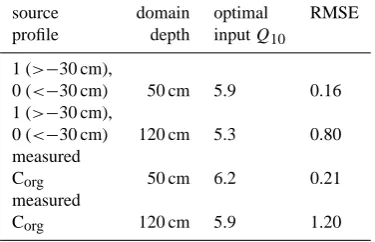
Table 2. Results of model validation under different settings.

source domain optimal RMSE

profile depth inputQ10

1 (>−30 cm),

0 (<−30 cm) 50 cm 5.9 0.16 1 (>−30 cm),

0 (<−30 cm) 120 cm 5.3 0.80 measured

Corg 50 cm 6.2 0.21

measured

Corg 120 cm 5.9 1.20

an Arrhenius relationship instead of the Q10 concept (not

shown). This also applies to all results shown below. The model fit was less good when using the measured, linearly interpolated Corg profile as a proxy of the source

strength distribution. Increasing the length of the model do-main to 120 cm also decreased model quality (Table 2). The optimal inputQ10values found for these different conditions

vary from 5.3 to 6.2, and would have been directly measured in depths between 10 cm and 20 cm. Considering CO2

dif-fusion either led to negligible differences or higher errors, depending on diffusivity (also see next sections).

3.3 Numerical experiments

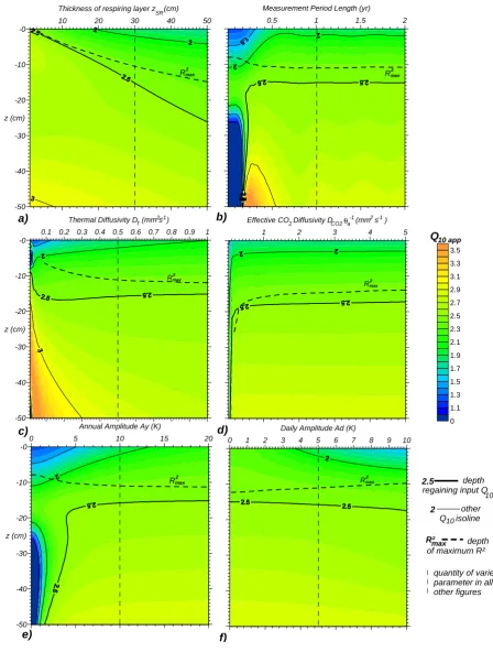
The validated model was used to study the effect of several factors on the apparentQ10 profile. Figure 3 shows

appar-entQ10 values as a function of both temperature

measure-ment depth and each factor considered in this study. The depth where theR2between soil respiration and temperature is highest is indicated withR_max2 . The inputQ10used to

gen-erate all plots is 2.5.

In the case of a homogenous respiring A-horizon of vary-ing thickness above a non-respirvary-ing subsoil (Fig. 3a), the inputQ10 is obtained at about half the depth of the

respir-ing layer. The highestR2, however, is found at a shallower depth. The difference between the optimal measurement depth and the depth with the highest correlation increases with the thickness of the respiring layer (up to 10 cm for a 50 cm thick respiring layer). The apparentQ10at the depth of

highestR2, however, does not differ more than 5% from the input value. Typical measurement depths used in field studies (0 to 10 cm) result in errors ranging from−30 to +10% de-pending on the depth of the respiring layer. The apparentQ10

values shown in Fig. 3a vary from less than 1.8 to more than 3, which is about the range of most reported values (Raich and Schlesinger, 1992), although the inputQ10was constant

at 2.5. In all other plots (Fig. 3b to f), we assumed a respiring layer thickness of 30 cm.

The impact of the length of the measurement period is il-lustrated in Fig. 3b. For short periods (less than about 180

days), the apparentQ10behaves highly irregular. For

mea-surement periods longer than a year, the apparentQ10is

sta-ble throughout the first 20 cm depth. It should be noted that we assumed that inter-annual variations in average tempera-ture can be neglected here. All other plots are based on a 1 year measurement period.

Changing the thermal diffusivity of the soil (one value for all depths, Fig. 3c), yields an irregular behaviour for values less than 0.1 mm2s−1. Above this threshold, possible ap-parentQ10 errors, as well as the distance between theQ10

obtained from the highestR2 and the inputQ10, decreases

with increasing diffusivity. We used a thermal diffusivity of 0.5 mm2s−1in all other plots.

The influence of CO2transport is neglected in all

simula-tions except for those presented in Fig. 3d. Considering gas diffusion leads to an offset in apparentQ10in the first 20 cm

compared to cases where diffusion is not considered, but the extent of this offset is less than 2% for effective diffusivities greater than 0.5 mm2s−1. Below 0.5 mm2s−1, this offset in-creases sharply and the depth of the highestR2can be found below rather than above the depth regaining the inputQ10.

In Fig. 3e, the annual temperature amplitude was varied from 0 to 20 K (twice the value used in the other model runs). For annual amplitudes below the diurnal amplitude of 5 K, the resulting profile is highly irregular with a local maximum. In addition, the temperature sensitivity is under-estimated throughout most of the modelling domain. Fig-ure 3f shows the effect of varying diurnal amplitudes. High diurnal amplitudes increase the errors made within the first 20 cm, and lead to an underestimation of temperature sensi-tivity when using shallow temperature sensors. Zero diurnal temperature amplitudes yield an almost linear apparentQ10

profile and a close proximity of the depth with the highestR2 and the inputQ10. Note that in our numerical experiments,

this behaviour could be reproduced using daily averages of temperature and CO2efflux. Averaging efflux before or

af-ter log-transformation only resulted in negligible differences (1Q10<0.01). Simulating only one measurement per day at

a fixed time also yields similar results, but with a small verti-cal offset of about 3 cm depending on the time of day of the measurement.

All experiments shown so far used a depth-invariant in-put sensitivity. Figure 4 shows the apparentQ10profiles

re-sulting from a linear change of inputQ10 between the

0.5 1 1.5 2 Measurement Period Length (yr)

depth of maximum R² depth regaining input Q d)

a) b)

c)

f)

-0

-10

-20

-30

-40

-50 z (cm)

10 20 30 40 50

Thickness of respiring layer z (cm)

Rmax2

SR

-0

-10

-20

-30

-40

-50 z (cm)

0.1 0.2 0.3 0.4 0.5 0.6 0.7 0.8 0.9 1

Thermal Diffusivity D (mm s )

R2 max

T 2 -1

1 2 3 4 5

Effective CO Diffusivity D (mm s )

R2

max

2 CO2 a -1 2 -1

Rmax2

0 1 2 3 4 5 6 7 8 9 10

Daily Amplitude Ad (K)

Rmax2

-0

-10

-20

-30

-40

-50 z (cm)

0 5 10 15 20

Annual Amplitude Ay (K)

Rmax2

e)

0 1.1 1.3 1.5 1.7 1.9 2.1 2.3 2.5 2.7 2.9 3.1 3.3 3.5 Q_{10 app}

θ

10 other Q isoline10

2.5

2

R²_max

quantity of varied parameter in all other figures

-50 -40 -30 -20 -10 0

1.7 2 2.3 2.6 2.9 3.2 3.5 3.8 4.1

Q₁₀

z

(

c

m

)

3.49 constant

3.55 constant

2.5 at surface, 4.6 at bottom

4.6 at surface, 2.5 at bottom 120 cm

respiring layer

30 cm respiring

layer

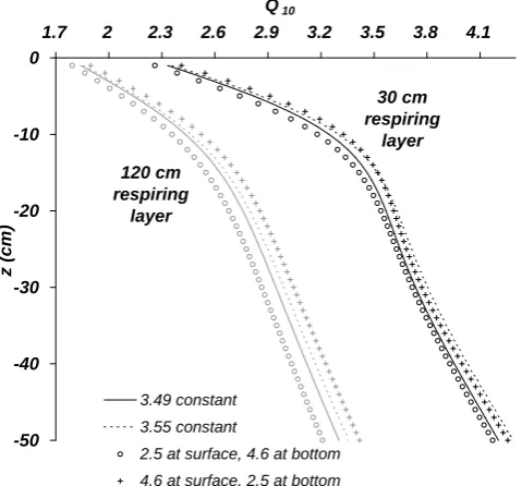
Fig. 4. ApparentQ10resulting from simulated hourly flux measure-ments as a function of temperature measurement depthzfor differ-ent linear inputQ10profiles (increasing and decreasing between 2.5 and 4.6) and thicknesses (30 cm and 120 cm) of the respiring layer.

identical results, differing mainly in aQ10offset of up to 0.21

in the upper 50 cm. The same is true for a depth-invariant Q10 that is the arithmetic (higher value) or geometric

aver-age of the above gradient in discrete 1 cm steps.

Figure 4 also shows the general effect of deep carbon (here, 120 cm) contributing the same reference temperature respiration as shallow horizons. In agreement with the trend in Fig. 3a, the depth regaining the inputQ10 moves further

downwards. All shown measurement depths now underesti-mate temperature sensitivity. A combination of this situation with a short measurement period or low annual amplitude (not shown) aggravates this underestimation, making local Q10 minima of less than 1 more probable. As a further

ex-ample of combinatory effects, a low thermal conductivity of 0.1 mm2s−1was combined with a varying measurement pe-riod. In this case, both very highQ10 above 10 and values

of less than 1 can be found in greater measurement depths, depending on the actual measurement period.

4 Discussion

4.1 Literature and own field measurements

The variability of theQ10dependence on temperature

mea-surement depth underlines the need for a methodology that allows comparison of temperature sensitivities determined in field experiments. Various explanations for the variability of apparentQ10profiles can be deduced from our modelling

ex-ercise. The highest reported apparentQ10 (Gaumont-Guay

et al., 2006) is based on those authors’ deepest temperature measurements and a short study period of two months. The amplitude of the diurnal temperature is strongly attenuated at that depth, and the amplitude of the annual cycle is not fully sampled because of the short measurement period. There-fore, CO2 efflux was correlated to temperature values with

small amplitude and high phase shift, which can result in very high or very low apparentQ10values. The even shorter

dataset by Pavelka et al. (2007) gives an example of such very low apparent sensitivities at great depths. At the same time, it yields very high values if the synchronization procedure sug-gested by the authors is applied. This procedure eliminates any phase shift, by gas diffusion or inadequate temperature measurement depth. The second highestQ10 increase with

depth (Khomik et al., 2006) originates from a study captur-ing the daily temperature cycle in summer, with additional less frequent measurements in spring and autumn, and no measurements in winter. The steep profiles found by Shi et al. (2006) and by ourselves were obtained for agricultural soils. A high and dense vegatation canopy, which is absent in these sites, attenuates the diurnal cycle more than the an-nual one. The diurnal cycle will be attenuated stronger with depth than the annual one. Therefore in agricultural soils, with a higher diurnal amplitude at the surface, larger changes of temperature with depth are detectable. The lowest increase ofQ10with depth was found in a study where measurements

of the diurnal cycle of CO2efflux were avoided (Wang et al.,

2006). The air temperature in proximity to the forest canopy included by Perrin et al. (2004) is supposed to have a higher diurnal amplitude than forest soil temperatures and conse-quently yields a lower apparentQ10.

4.2 Model validation

The model application to the field data demonstrates that the model is able to describe the temperature sensitivity varia-tion with depth. The remaining uncertainty of about±10% occurs when considering deeper layers, and their carbon con-tent (Table 2). We attribute this to two main causes. First, temperature measurement errors become increasingly signif-icant deeper in the soil, where amplitudes are smaller. Such errors are not simulated by the model. However, tempera-ture sensitivity of soil respiration is rarely determined from temperature sensors installed in large depths. Second, there is considerable uncertainty in the source strength distribu-tion. Organic carbon content includes accumulated stable carbon pools, the fraction of which can be depth-dependent itself. The field data were best described when neglecting the organic carbon content found below the A-horizon. This seems to indicate that deeper carbon is less involved in respi-ration activity, which is in good agreement with the general assumption that carbon pools in deeper horizons are more stable (cf. Fierer et al., 2003). The increasing uncertainty with depth also implies that field measurements of CO2

ef-flux at the soil surface are not suited to derive the temperature sensitivity of deep buried carbon, which has been associated with higher temperature sensitivities by some (Knorr et al., 2005; Davidson and Janssens, 2006). Recently, an additional sensitivity of deep carbon decomposition to fresh carbon sup-ply has been suggested (Fontaine et al., 2007). Our study shows that although a true increase ofQ10 with depth may

be present, it should not be confused with the temperature measurement depth dependence of the apparentQ10(also see

Fig. 4).

It was not necessary to consider CO2 diffusion to model

the apparentQ10 variation with depth for our field

experi-ment. This fits well with the results of the numerical exper-iments discussed in the next section, which showed that for most diffusivities observed in the field the impact should be low (Fig. 3d; Tang et al., 2003; Werner et al., 2004). Nev-ertheless, a general recommendation to neglect CO2

trans-port should not be made based on the results of a single field study.

It is noteworthy that the measurement depths that would have yielded aQ10 value in the range of the optimal input Q10 of the model, are below 10 cm, while all single

mea-surement depths found in our literature study are above that depth. When modelling a whole year, the apparentQ10

dif-fers less than 7% in the upper 30 cm and up to 16% in 50 cm depth. Given the ability of the model to describe the data measured during 10 months correctly, we assume that a full one-year dataset of hourly respiration would have shown the same deviation.

Finally, it should be mentioned that the model only con-siders the pure confounding factor temperature measurement depth. Depending on the site characteristics, other confound-ing effects, such as correlation of temperature with soil

mois-ture (Davidson et al., 1998), may cause errors of similar mag-nitude in field-basedQ10 determination. In most climates,

this correlation is negative, resulting in a further underes-timation if CO2 production is moisture-limited. However,

Davidson et al. (2006) also demonstrated cases where the availability of other substrates may lead to an overestimation, e.g. oxygen influenced by moisture. Such other confounding factors may be responsible for the highQ10we found after

correcting for measurement depth errors. As already stated, the model does not consider root respiration. Therefore, tem-perature measurement depth errors in soils with a consider-able contribution of roots can only be described correctly if other factors controlling root-related respiration do not co-vary with temperature. This problem was already discussed in the previous section. Also, roots may contribute to the va-riety of temperature sensitivities found in a single site or even depth. Boone et al. (1998) found strongly differing temper-ature responses between heterotrophic and root-related (in-cluding exudation-driven heterotrophic) respiration (cf. next section).

4.3 Numerical experiments

When the vertical source strength distribution consists of a homogenous respiring layer above a non-respiring sub-soil, the best depth to place a single temperature sensor is the cen-tre of the respiring layer (Fig. 3a). Although such a distribu-tion is not unrealistic for our field reference dataset, it may be not fulfilled in non-agricultural soils, especially in the pres-ence of litter layers. As an alternative method to determine the most appropriate depth, Tang et al. (2003), Perrin et al. (2004), Shi et al. (2006) and Pavelka et al. (2007) suggested the maximumR2criterion. Although our numerical exper-iments show that this is not exactly correct, it is a good ap-proximation in most conditions. However, both theR2 crite-rion and the centre placement fail in extreme conditions, as illustrated in Fig. 3b to e.

The difference between the depth of highestR2 and the depth regaining the inputQ10is a result of the combined

ef-fect of amplitude attenuation and phase shift of temperature waves. For an infinitely thin respiring layer, theR2is high-est for a temperature measurement within this layer. This measurement will also provide the correct Q10. At other

depths, theR2is lower due to phase shifts in the temperature time series. For thicker respiring layers, efflux at the sur-face integrates over CO2production time series with

differ-ent delays and amplitudes. If the delay is considered in isola-tion, the highestR2would occur in the middle of the respir-ing layer. However, the apparentQ10would underestimate

the depth of highestR2is shifted upwards. At the same time, the lower temperature amplitudes in these depths counteract the underestimation of the apparentQ10. Strictly spoken, the

temperature measurement depth regaining the inputQ10 is

not a “correct” depth, but a depth where positive and nega-tive errors are balanced.

The depth that regains the inputQ10 will not always be

within the respiring layer, as illustrated by Fig. 3b. In this figure, the length of the measurement period was varied. The model qualitatively confirms that extremely high appar-ent temperature sensitivities for greater measuremappar-ent depths, such as those found by Gaumont-Guay et al. (2006) and Khomik et al. (2006), can be caused by incomplete repre-sentation of the annual cycle. For a more quantitative as-sessment, too little is known especially on the varying thick-ness and thermal properties of the snow cover, which was an important feature in both studies. Organic topsoils were reported from both studies, which may have had a very low thermal diffusivity. According to our model, this can lead to highly irregular apparentQ10profiles. The fact that

measure-ment periods of less than half a year can result in highQ10

errors is also relevant to studies separating the study period into seasons to capture plant phenological effects on temper-ature sensitivity (e.g. Xu and Qi, 2001; Yuste et al., 2004; deForest et al., 2006). The model also demonstrates that for even shorter measurement periods, such as the one analyzed by Pavelka et al. (2007), great measurement depths can yield very low apparent sensitivities.

Variation of the soil thermal diffusivity (Fig. 3c) confirms the expectation that accurate field-basedQ10 measurements

are more likely when temperature waves propagate rapidly into the ground. According to Zmarsly et al. (2002), most soils have thermal diffusivities ranging between 0.1 (dry or-ganic) and 0.75 mm2s−1(wet sand). Therefore, the irregular behaviour of the apparentQ10 for very low diffusivities is

not relevant in most ecosystems.

Effective CO2diffusivities can cover a much larger range.

A compilation of Werner et al. (2004) based on 81 stud-ies shows thatDCO2θ

−1

a can range from 0.09 to more than 12 mm2s−1. Despite this large range, our numerical experi-ment shows that the influence of diffusion on apparentQ10

would be negligible for all but the three lowest values sum-marized by Werner et al. (2004). It is interesting that for such small diffusivities, the depth of highestR2 can drop below the depth regaining the inputQ10. We attribute this to the fact

that the time series of surface efflux is now delayed compared to the temperature time series in those depths where most of the CO2is produced. Consequently, efflux correlates better

with deeper temperature time series. This is no indication of a causal relationship, as the CO2produced in these depths is

delayed even stronger before reaching the surface.

An evaluation of the effect of annual temperature ampli-tude (Fig. 3e) is relevant to avoid systematic errors when tem-perature sensitivities from different climatic zones are com-pared. Close to the equator where the annual amplitude is

low, field-based determination of accurateQ10values is

dif-ficult. Typically, the temperature sensitivity will be under-estimated. Continental and boreal climates with high annual amplitudes potentially allow an accurate determination of the Q10 when the measurement period is long and continuous.

This may be difficult in case of harsh winter conditions, or be complicated by the thermal properties of a snow cover (see above).

The numerical experiment on diurnal amplitude (Fig. 3f) is of particular interest because the positive effects of low diurnal amplitudes can be approximated by daily averaging of efflux and temperature time series. A similar reduction in daily amplitude can be obtained by measurements at a fixed time of day, but it remains to be examined whether this alter-native is more susceptible to varying day lengths and ampli-tudes throughout the year.

The experiment on depth-variant inputQ10confirms what

has been discussed during the model validation: Surface ef-flux measurements are poorly suited to assess the vertical variability of temperature sensitivity. TheQ10derived from

such a field study, even if the correct measurement depth was chosen, only represents an effective mean of the potentially different sensitivities of soil horizons. It remains to be tested whether additional CO2concentration measurements in

var-ious depths, or varying vertical profiles of soil moisture, can solve this ambiguity problem.

In general, our analyses indicate that a temperature mea-surement depth within the upper 10 cm, as commonly used in field studies, is likely to result in an underestimation of tem-perature sensitivity, at least in the absence of a litter layer. According to the latest IPCC report (Solomon et al., 2007), most models used to estimate the biochemical feedback of land surfaces to climate change assume a soil respirationQ10

close to 2. It is noteworthy that this assumption is based on averaging not only laboratory but also field studies (Solomon et al., 2007), e.g. those compiled by Raich and Schlesinger (1992). These models predict a global effective sensitivity of heterotrophic respiration of 6.2% per K warming. How-ever, a largerQ10of 2.5 would be well within the uncertainty

range identified in this study. This would increase global sen-sitivity by about one third in each model, which is the same order of magnitude as the standard deviation among the mod-els. The models give an average absolute sensitivity of land surfaces to climate change of−79 Gt sequestered carbon per K warming, although this rate is highly variable between the models (±45 GtC K−1_{). An additional uncertainty of one}

5 Conclusions

We described the development, validation, and application of a simple model to explain and estimate the errors in tem-perature sensitivity determination related to the temtem-perature measurement depth. We chose the widely usedQ10concept

as an example, but the alternative activation energy concept provides almost identical results.

Depending on study conditions, the vertical profile of the apparentQ10 may range from fairly regular to highly

irreg-ular. The latter case can include local minima and maxima, decoupling of the depth of correct Q10 from the depth of

highestR2, and cases where the obtainedQ10is incorrect for

all conventional temperature measurement depths. In these cases, only laboratory incubation experiments directly can yield correct temperature sensitivity relations, although these experiments are not free of errors and assumptions either. An alternative possibility would be to inversely estimate theQ10

using numerical models of CO2production, CO2 transport

and heat transport applied to field data. This approach has recently been used to estimate soil physical properties and CO2source strength (Herbst et al., 2008; Novak, 2007;

Wei-herm¨uller et al., 2008) and could be extended toQ10

estima-tion in future.

In many field studies, however, the detailed input data re-quired to drive mechanistic CO2models are not available. In

such cases, the model presented here, and some basic climate and soil data, may help reducing errors in temperature sen-sitivity analysis. Nevertheless, validation has shown that an uncertainty remains due to the choice of input parameters. Also, analyses of additional field data sets to test whether the simplifications made within the model are justified would be desirable. Ideally, a model to asses the effect of temperature measurement depth, as of other confounding factors, would accompany each field study. However, careful interpretation of the results presented here may provide some general con-clusions which kind of conditions are favourable to reduce measurement depth errors. These are:

– a thin and easily distinguished horizon of respiration ac-tivity,

– a high thermal and CO2diffusivity of the soil, – a high annual temperature amplitude,

– a measurement period of one year or more,

– daily averaging of measurements before fitting the tem-perature sensitivity function.

Note that the last two conditions may be in conflict with other confounding factors that require short measurement pe-riods, such as moisture or phenology-dependentQ10

mea-surements.

In the conditions identified above, the bias introduced by the maximumR2depth method used by some authors will be

small. In some cases, the aim of determining a temperature sensitivity is empirical modelling, e.g. for gap-filling, rather than inter-site comparison or process-based modelling. In this case, error minimization by choosing the depth of maxi-mumR2may be advantageous.

Appendix A

Temperature sensitivity functions

Two methods are most commonly used to relate temperature and respiration. The first is an empirical exponential rela-tionship suggested by van t’Hoff (e.g. Yuste et al., 2004):

SR=SRTrefe lnQ₁₀

10 (T−Tref) _(A1)

whereSR is soil respiration (µmol m−2s−1),T is tempera-ture (K) andTrefis an arbitrary reference temperature with a

know respiration rateSRTref.Q10 is the rate by which

respi-ration changes with a temperature change of 10 K. TheQ10

is a commonly used parameter to report the temperature sen-sitivity of soil respiration. The second relationship is more physically based and uses activation energy considerations introduced by Arrhenius (e.g. Lloyd and Taylor, 1994):

SR=SRTrefe

Ea

R T Tref(T−Tref) _(A2)

Here, Ea is the activation energy (J mol−1), and R=8.314 J mol−1_K−1 _{is the universal gas constant.}

Further temperature sensitivity functions are summarised by K¨atterer et al. (1998), Bauer et al. (2008) and Tuomi et al. (2008). The temperature sensitivity coefficients of these methods (Q10andEa) are not equivalent. For typical temperature and respiration ranges, a Q10 value derived

from Eq. (A2) based onEadecreases slowly with increasing temperature, whereasQ10is a constant in Eq. (A1). A slow Q10decrease with increasing temperature has been reported

Appendix B

Theory of soil temperature profiles

Soil surface temperature changes are mainly induced by the radiation balance at the soil surface and exchange of sensi-ble and latent heat between the soil and the atmosphere. The variation in soil surface temperature propagates into deeper layers. In the absence of transport of sensible and latent heat in the soil gas phase (Weber et al., 2007), this process is con-trolled by the soil thermal diffusivityDT (m2s−1):

∂T ∂t =DT

∂2T

∂z2 = λ ρc

∂2T

∂z2 (B1)

wheret is time (s) andzis depth (m). Thermal diffusivity is a function of thermal conductivityλ (W m−1K−1), heat capacityc(J kg−1K−1), and bulk densityρ (kg m−3). The typical order of magnitude of soil thermal diffusivity is 10−7 to 10−6m2s−1(Zmarsly et al., 2002). To transfer a soil tem-perature time series to another depth, it is often represented by a series of sine waves (van Wijk, 1963; Verhoef et al., 1996; Heusinkveld et al., 2004; Graf et al., 2008):

T =T + n

X

i=1 Aisin

2π(t+1ti) τi

(B2) whereT denotes the average temperature (K),Aiis the tem-perature amplitude (K),τi is the period length (s), and1ti the phase shift (here in units of time and therefore included in the bracketed term) of the sine wave indexedi. When thermal diffusivity is constant with depth and time, there is an analytical solution to Eqs. (B1) and (B2) (van Wijk, 1963) that predicts temperature in any other depth (Heusinkveld et al., 2004; Graf et al., 2008):

T =T + n

X

i=1 Aiexp

1z

r _π

DTτi

sin

2π(t+1ti+1zτ2πi

q _π

DTτi)

τi

(B3) where1zis the difference between the actual and the refer-ence depth.

Stepwise application of Eq. (B3) allows to treat thermal diffusivities that change along a vertical profile (cf. meth-ods section). However, it should be noted that for such an effective thermal diffusivity in soils with a vertical change of thermal properties, the simple relation betweenλ,cand DT given in Eq. (B1) is no longer valid. Nassar and Horton (1989) describe a method yielding an effective diffusivity for numerical forward modelling. If no temperature time series from different depths in the field are available, butλandc as determined in laboratory or estimated from literature sig-nificantly vary with depth, both approaches do not work. In this case, either a numerical model treating storage and dif-fusion separately has to be used, or a more complex analyt-ical model considering the vertanalyt-ical profile of bothλ andc.

Such models for specific, regular vertical profiles have been summarized and tested by Massman (1993). An even more general approach, which allows for any profile of thermal properties to be resolved in discrete stpes of e.g. 1 cm and is therefore well compatible with our model, has been sug-gested by Karam (2000).

Appendix C

Theory of gas diffusion

The dynamics of CO2in soil air is described by: ∂c

∂t =τ θaDa ∂2ca

∂z2 +SR (C1)

wherecis the total volumetric concentration of CO2,ca is the concentration in soil air,Da is the diffusivity of CO2in

air (m2s−1_{), θ}

a (dimensionless) is the soil air content, and τ is a dimensionless tortuosity factor. Da, the soil air con-tent, tortuosity and other factors such as transport through soil water and pressure turbulence can be combined into an effective diffusivity (Simunek and Suarez, 1993; Hirano et al., 2003; Tang et al., 2003; Takle et al., 2004). In this study, we use a wide range of field-determined effective diffusivi-ties reviewed by Werner et al. (2004). To solve Eq. (C1), we use an explicit time discretization:

c(t+1t, z)= c(t, z)+1t (SR(t, z)

+DCO2(z−

1 21z)

c(t,z−1z)−c(t,z) θa1z2

−DCO2(z+

1 21z)

c(t,z)−c(t,z+1z)

θa1z2 ) (C2)

By definingDCO2 in planes 0.51zabove and below all other

depth-dependent input data, we achieve mass-consistency. The maximum value of the time-step for a stable solution is1t <0.51z2D_CO−1

2θa.

Acknowledgements. We gratefully acknowledge field assistance

by Rainer Harms, partial funding of A. Graf’s postdoctoral appointment by the “Impuls- und Vernetzungsfonds” of the Helmholtz Association, financial support by the Helmholtz-funded FLOWatch project and by the SFB/TR 32 “Patterns in Soil-Vegetation-Atmosphere Systems: Monitoring, Modelling, and Data Assimilation” funded by the Deutsche Forschungsgemeinschaft (DFG), and helpful comments by all participants of the BGD open discussion related to this publication.

Edited by: J. Leifeld

References

Bauer, J., Herbst, M., Huisman, J. A., Weiherm¨uller, L., and Vereecken, H.: Sensitivity of simulated soil heterotrophic res-piration to temperature and moisture reduction functions, Geo-derma, 145, 17–27, 2008.

Boone, R. D., Nadelhoffer, K. J., Canary, J. D., and Kaye, J. P.: Roots exert a strong influence on the temperature sensitivity of soil respiration, Nature, 396, 570–572, 1998.

Borken, W., Davidson, E. A., Savage, K., Gaudinski, J., and Trum-bore, S. E.: Drying and wetting effects on carbon dioxide release from organic horizons, Soil Sci. Soc. Am. J., 67, 1888–1896, 2003.

Chen, X. Y., Eamus, D., and Hutley, L. B.: Seasonal patterns of soil carbon dioxide efflux from a wet-dry tropical savanna of northern Australia, Aust. J. Bot., 50, 43–51, 2002.

Conen, F., Leifeld, J., Seth, B., and Alewell, C.: Warming min-eralises young and old carbon equally, Biogeosciences, 3, 515– 519, 2006,

http://www.biogeosciences.net/3/515/2006/.

Davidson, E. A. and Janssens, I. A.: Temperature sensitivity of soil carbon decomposition and feedbacks to climate change, Nature, 440, 165–173, 2006.

Davidson, E. A., Belk, E., and Boone, R. D.: Soil water content and temperature as independent or confounded factors controlling soil respiration in a temperate mixed hardwood forest, Global Change Biol., 4, 217–227, 1998.

Davidson, E. A., Janssens, I. A., and Luo, Y.: On the variability of respiration in terrestrial ecosystems: moving beyondQ10, Glob. Change Biol., 12, 154–164, 2006.

deForest, J. L., Noormets, A., McNulty, S. G., Sun, G., Tenney, G., and Chen, J.: Phenophases alter the soil respiration-temperature relationship in an oak-dominated forest, Int. J. Biometeorol., 51, 135–144, 2006.

Dugas, W. A.: Micrometeorological and Chamber Measurements of CO2Flux from Bare Soil, Agr. Forest Meteorol., 67, 115–128, 1993.

Fang, C., Moncrieff, J. B., Gholz, H. L., and Clark, K. L.: Soil CO2 efflux and its spatial variation in a Florida slash pine plantation, Plant Soil, 205, 135–146, 1998.

Fang, C. M., Smith, P., Moncrieff, J. B., and Smith, J. U.: Simi-lar response of labile and resistant soil organic matter pools to changes in temperature, Nature, 433, 57–59, 2005.

Fierer, N., Allen, A. S., Schimel, J. P., and Holden, P.: Controls on microbial CO2production: a comparison of surface and subsur-face horizons, Global Change Biol., 9, 1322–1332, 2003. Fontaine, S., Barot, S., Barre, P., Bdioui, N., Mary, B., and Rumpel,

C.: Stability of organic carbon in deep soil layers controlled by fresh carbon supply, Nature, 450, 277–281, 2007.

Gaumont-Guay, D., Black, T. A., Griffis, T. J., Barr, A. G., Jassal, R. S., and Nesic, Z.: Interpreting the dependence of soil respiration on soil temperature and water content in a boreal aspen stand, Agr. Forest Meteorol., 140, 220–235, 2006.

Graf, A., Kuttler, W., and Werner, J.: Mulching as means to exploit dewfall for arid agriculture?, Atmos. Res., 87, 369–376, 2008. Hanson, P. J., Edwards, N. T., Garten, C. T., and Andrews, J. A.:

Separating root and soil microbial contributions to soil respira-tion: A review of methods and observations, Biogeochemistry, 48, 115–146, 2000.

Hashimoto, S. and Komatsu, H.: Relationships between soil CO₂ concentration and CO2production, temperature, water content,

and gas diffusivity: implications for field studies through sensi-tivity analyses, J. Forest Res.-JPN, 11, 41–50, 2006.

Herbst, M., Hellebrand, H. J., Bauer, J., Huisman, J. A., Simunek, J., Weiherm¨uller, L., Graf, A., Vanderborght, J., and Vereecken, H.: Multiyear heterotrophic soil respiration: evaluation of a cou-pled CO2 transport and carbon turnover model, Ecol. Model., 214, 271–283, 2008.

Heusinkveld, B. G., Jacobs, A. F. G., Holtslag, A. A. M., and Berkowicz, S. M.: Surface energy balance closure in an arid re-gion. Role of soil heat flux, Agr. Forest Meteorol., 122, 21–37, 2004.

Hirano, T., Kim, H., and Tanaka, Y.: Long-term half-hourly mea-surement of soil CO2concentration and soil respiration in a tem-perate deciduous forest, J. Geophys. Res. Atmos., 108(D20), 4631, doi:10.1029/2003JD003766, 2003.

Humphreys, E. R., Black, T. A., Morgenstern, K., Cai, T. B., Drewitt, G. B., Nesi, Z., and Trofymow, J. A.: Carbon dioxide fluxes in coastal Douglas-fir stands at different stages of develop-ment after clearcut harvesting, Agr. Forest Meteorol., 140, 6–22, 2006.

Karam, M. A.: A thermal wave approach for heat transfer in a nonuniform soil, Soil Sci. Soc. Am. J., 64, 1219–1225, 2000. K¨atterer, T., Reichstein, M., Andr´en, O., and Lomander, A.:

Tem-perature dependence of organic matter decomposition: a critical review using literature data analyzed with different models, Biol. Fert. Soils, 27, 258–262, 1998.

Khomik, M., Arain, M. A., and McCaughey, J. H.: Temporal and spatial variability of soil respiration in a boreal mixedwood for-est, Agr. Forest Meteorol., 140, 244–256, 2006.

Kim, J. and Verma, S. B.: Soil CO2flux in a Minnesota peatland, Biogeochemistry, 18, 37–51, 1992.

Kirschbaum, M. U. F.: The temperature dependence of organic-matter decomposition – still a topic of debate, Soil Biol. Biochem., 38, 2510–2518, 2006.

Knorr, W., Prentice, I. C., House, J. I., and Holland, E. A.: Long-term sensitivity of soil carbon turnover to warming, Nature, 433, 298–301, 2005.

Larinova, A. A., Yevdokimov, I. V., and Bykhovets, S. S.: Tempera-ture response of soil respiration is dependent on concentration of readily decomposable C, Biogeosciences, 4, 1073–1081, 2007, http://www.biogeosciences.net/4/1073/2007/.

Law, B. E., Falge, E., Gu, L., et al.: Environmental controls over carbon dioxide and water vapor exchange of terrestrial vegeta-tion, Agr. Forest Meteorol., 113, 97–120, 2002.

Lloyd, J. and Taylor, J. A. On the temperature-dependence of soil respiration, Funct. Ecol., 8, 315–323, 1994.

Lou, Y. S., Li, Z. P., and Zhang, T. L.: Soil CO2 flux in relation to dissolved organic carbon, soil temperature and moisture in a subtropical arable soil of China, J. Environ. Sci.-China, 15, 715– 720, 2003.

Massman, W. J.: Periodic temperature variations in an inhomoge-neous soil: a comparison of exact and analytical expressions, Soil Sci., 155, 331–338, 1993.

Moyano, F. E., Kutsch, W. L., and Rebmann, C.: Soil respiration fluxes in relation to photosynthetic activity in broad-leaf and needle-leaf forest stands, Agr. Forest Meteorol., 148, 135–143, 2008.

Novak, M. D.: Determination of soil carbon dioxide source-density profiles by inversion from soil-profile gas concentrations and sur-face flux density for diffusion-dominated transport, Agr. Forest Meteorol., 146, 189–204, 2007.

Novick, K. A., Stoy, P. C., Katul, G. G., Ellsworth, D. S., Siqueira, M. B. S., Juang, J., and Oren, R.: Carbon dioxide and water vapor exchange in a warm temperate grassland, Oecologia, 138, 259–274, 2004.

Pavelka, M., Acosta, M., Marek, M. V., Kutsch, W., and Janous, D.: Dependence of the Q10 values on the depth of the soil tempera-ture measuring point, Plant Soil, 292, 171–179, 2007.

Perrin, D., Laitat, E., Yernaux, M., and Aubinet, M.: Modelling the response of forest soil respiration fluxes to the main climatic variables, Biotechnol. Agron. Soc. Environ., 8, 15–25, 2004. Raich, J. W. and Schlesinger, W. H.: The global carbon dioxide flux

in soil respiration and its relationship to vegetation and climate, Tellus, 44(B), 81–99, 1992.

Reichstein, M. and Beer, C.: Soil respiration across scales: The importance of a model-data integration framework for data inter-pretation, J. Plant Nutr. Soil Sci., 171, 1–11, 2008.

Reichstein, M., Subke, J. A., Angeli, A. C., and Tenhunen, J. D.: Does the temperature sensitivity of decomposition of soil organic matter depend upon water content, soil horizon, or incubation time?, Glob. Change Biol., 11, 1754–1767, 2005a.

Reichstein, M., K¨atterer, T., Andr`en, O., Ciais, P., Schulze, E. D., Cramer, W., Papale, D., and Valentini, R.: Temperature sensi-tivity of decomposition in relation to soil organic matter pools: critique and outlook, Biogeosciences, 2, 317–321, 2005b, http://www.biogeosciences.net/2/317/2005/.

Sanderman, J., Amundson, R. G., and Baldocchi, D. D.: Applica-tion of eddy covariance measurements to the temperature depen-dence of soil organic matter mean residepen-dence time, Global Bio-geochem. Cy., 17, 1061, doi:10.1029/2001GB001833, 2003. Savage, K. E. and Davidson, E. A.: A comparison of manual and

automated systems for soil CO₂flux measurements: trade-offs between spatial and temporal resolution, J. Exp. Bot., 54, 891– 899, 2003.

Shi, P. L., Zhang, X. Z., Zhong, Z. M., and Ouyang, H.: Diurnal and seasonal variability of soil CO2efflux in a cropland ecosystem on the Tibetan Plateau, Agr. Forest Meteorol., 137, 220–233, 2006. Simunek, J. and Suarez, D. L.: Modeling of carbon-dioxide trans-port and production in soil. 1. Model development, Water Resour. Res., 29, 487–497, 1993.

Solomon, S., Qin, D., Manning, M., et al. (Eds.): Climate Change 2007: The Physical Science Basis, Contribution of Working Group I to the Fourth Assessment Report of the Intergovern-mental Panel on Climate Change Cambridge University Press, Cambridge, United Kingdom and New York, NY, USA, 501– 539, 2007.

Takahashi, A., Hiyama, T., Takahashi, H. A., and Fukushima, Y.: Analytical estimation of the vertical distribution of CO₂ produc-tion within soil: applicaproduc-tion to a Japanese temperate forest, Agr. Forest Meteorol., 126, 223–235, 2004.

Takle, E. S., Massmann, W. J., Brandle, J. R., et al.: Influence of high-frequency ambient pressure pumping on carbon dioxide ef-flux from soil, Agr. Forest Meteorol., 124, 193–206, 2004.

Tang, J. W., Baldocchi, D. D., Qi, Y., and Xu, L. K.: Assessing soil CO2efflux using continuous measurements of CO2profiles in soils with small solid-state sensors, Agr. Forest Meteorol., 118, 207–220, 2003.

Tang, J. W., Baldocchi, D., and Xu, L. K.: Tree photosynthesis modulates soil respiration on a diurnal time scale, Global Change Biol., 11, 1298–1304, 2005.

Tang, J., Bolstad, P. V., Desai, A. R., Martin, J. G., Cook, B. D., Davis, K. J., and Carey, E. V.: Ecosystem respiration and its com-ponents in an old-growth forest in the Great lakes region of the United States, Agric. For. Meteorol., 148, 171–185, 2008. Tuomi, M., Vanhala, P., Karhu, K., Fritze, H., and Liski, J.:

Het-erotrophic soil respiration - Comparison of different models de-scribing its temperature dependence, Ecol. Model., 211, 182– 190, 2008.

van Wijk, W. R. (Ed.): Physics of Plant Environment, North Hol-land, Amsterdam, The Netherlands, p. 133–134, 1963.

Verhoef, A., van den Hurk, B. J. J. M., Jacobs, A. F. G., and Heusinkveld, B. G.: Thermal soil properties for vineyard (EFEDA-I) and savanna (HAPEX-Sahel) sites, Agr. Forest Me-teorol., 78, 1–18, 1996.

Wang, C., Yang, J., and Zhang, Q.: Soil respiration in six temperate forests in China, Global Change Biol., 12, 2103–2114, 2006. Weber, S., Graf, A., and Heusinkveld, B. G.: Accuracy of soil heat

flux plate measurements in coarse substrates – Field measure-ments versus a laboratory test, Theor. Appl. Climatol., 89, 109– 114, 2007.

Weiherm¨uller, L., Huisman, J. A., Lambot, S., Herbst, M., and Vereecken, H.: Mapping the spatial variation of soil water con-tent at the field scale with different ground penetrating radar tech-niques, J. Hydrol., 340, 205–216, 2007.

Weiherm¨uller, L., Huisman, J. A., Graf, A., Herbst, M., and Se-quaris, J.-M.: Multistep outflow experiments for the simultane-ous determination of soil physical and CO2production parame-ters, Vadose Zone J., in press, 2008.

Werner, D., Grathwohl, P., and H¨ohener, P.: Review of field meth-ods for the determination of the tortuosity and effective gas-phase diffusivity in the vadose zone, Vadose Zone J., 3, 1240–1248, 2004.

Xu, M. and Qi, Y.: Spatial and seasonal variations ofQ10 deter-mined by soil respiration measurements at a Sierra Nevada for-est, Global Biogeochem. Cy., 15, 687–696, 2001.

Yuste, J. C., Janssens, I. A., Carrara, A., and Ceulemans, R.: Inter-active effects of temperature and precipitation on soil respiration in a temperate maritime forest, Tree Physiol., 23, 1263–1270, 2003.

Yuste, J. C., Janssens, I. A., Carrara, A., and Ceulemans, R.: Annual Q(10) of soil respiration reflects plant phenological patterns as well as temperature sensitivity, Global Change Biol., 10, 161– 169, 2004.