Mound slope and shape selection during unstable multilayer growth: Analysis of step-dynamics models including downward funneling

Physics and Astronomy Publications

Physics and Astronomy

3-2006

Mound slope and shape selection during unstable

multilayer growth: Analysis of step-dynamics

models including downward funneling

Maozhi Li

Iowa State University

James W. Evans

Iowa State University, [email protected]

Follow this and additional works at:

http://lib.dr.iastate.edu/physastro_pubs

Part of the

Biological and Chemical Physics Commons

, and the

Mathematics Commons

The complete bibliographic information for this item can be found athttp://lib.dr.iastate.edu/physastro_pubs/202. For information on how to cite this item, please visithttp://lib.dr.iastate.edu/howtocite.html.

Analysis of step-dynamics models including downward funneling

Abstract

Step-dynamics models are developed for mound shape evolution during multilayer homoepitaxial growth in

the presence of inhibited interlayer transport. Unconventionally, our models also incorporate downward

funneling (DF) of atoms deposited at step edges. The extent of DF can be reduced continuously to zero where

one recovers traditional step dynamics models. This allows direct comparison between the behavior of models

with and without DF. We show that DF greatly enhances growth of the height of valleys at the mound bases to

an extent compatible with slope selection. To elucidate the selected shapes of finite mounds, we consider a

suitably defined net flux of adatom attachment at steps summed over a mound side between valley and peak.

This quantity varies periodically but vanishes when further averaged over time, a condition which directly

constrains the selected mound shapes. We also characterize the dependence of these shapes on the

prescription of nucleation of new islands at the mound peak.

Disciplines

Biological and Chemical Physics | Mathematics

Comments

This article is from

Physical Review B

73 (2006): 125434, doi:

10.1103/PhysRevB.73.125434

. Posted with

permission.

Mound slope and shape selection during unstable multilayer growth:

Analysis of step-dynamics models including downward funneling

Maozhi Li1and J. W. Evans2

1_{Institute of Physical Research and Technology, and Ames Laboratory⫺USDOE, Iowa State University, Ames, Iowa 50011, USA} 2_{Department of Mathematics, and Ames Laboratory⫺USDOE, Iowa State University, Ames Iowa 50011, USA}

共Received 16 November 2005; published 28 March 2006兲

Step-dynamics models are developed for mound shape evolution during multilayer homoepitaxial growth in the presence of inhibited interlayer transport. Unconventionally, our models also incorporate downward fun-neling共DF兲of atoms deposited at step edges. The extent of DF can be reduced continuously to zero where one recovers traditional step dynamics models. This allows direct comparison between the behavior of models with and without DF. We show that DF greatly enhances growth of the height of valleys at the mound bases to an extent compatible with slope selection. To elucidate the selected shapes of finite mounds, we consider a suitably defined net flux of adatom attachment at steps summed over a mound side between valley and peak. This quantity varies periodically but vanishes when further averaged over time, a condition which directly constrains the selected mound shapes. We also characterize the dependence of these shapes on the prescription of nucleation of new islands at the mound peak.

DOI:10.1103/PhysRevB.73.125434 PACS number共s兲: 68.55.⫺a, 81.10.Aj, 81.15.Aa, 68.35.Fx

I. INTRODUCTION

The morphological evolution of thin films during epitaxial growth is a topic of fundamental and technological interest. Even for homoepitaxial growth, the interplay between depo-sition of atoms and various inhibited surface diffusion pro-cesses gives rise to a rich variety of far-from-equilibrium surface morphologies.1,2 _{In homoepitaxy, atoms are} depos-ited onto and diffuse across the surface, and then aggregate into two-dimensional 共2D兲 islands. For atoms subsequently deposited on top of islands, there typically exists an addi-tional Ehrlich-Schwoebel 共ES兲 step edge barrier inhibiting interlayer transport.3,4 _{The presence of such an ES barrier} leads to unstable film growth characterized by kinetic rough-ening and the formation of three-dimensional共3D兲mounds, i.e., multilayer stacks of 2D islands.

This unstable growth mode was explained by Villain as follows.5,6_{The presence of an ES barrier implies that} diffus-ing atoms tend to be reflected from descenddiffus-ing steps and incorporated into ascending steps. This diffusion bias pro-duces a destabilizing lateral mass current in the uphill direc-tion. A number of homoepitaxial growth experiments have revealed not only mounded morphologies, but also suggested the development of a well-defined selected mound slope fol-lowing a regime of steepening of mound sides.7–11_{The latter} feature has been associated with the presence of nonthermal dynamical processes related to the downward transport of atoms deposited near step edges.12–15_{One example of such a} process is “downward funneling” 共DF兲.16–18 _Molecular dy-namics simulations reveal that atoms deposited at step edges or on the sides of multilayer nanoprotrusions in metal共100兲 systems16,19–21 _{or metal共111兲 systems}22 _{funnel down to} fourfold-hollow or threefold-hollow adsorption sites, respec-tively, in lower layers. Unstable growth behavior has been explored utilizing kinetic Monte Carlo simulation of both generic and realistic atomistic lattice-gas models with con-siderable emphasis on the slow coarsening of mound dimen-sions following slope selection.11,14,15,23,24

Simulation of realistic atomistic models can provide a de-tailed picture of the evolution of thin film morphologies, and comparison with experiment facilitates determination of key energetic parameters.11,13,15_{However, this approach does not} necessarily provide a clear elucidation of the subtle coopera-tive aspects of morphological evolution during film growth, e.g., the dynamics of mound steepening or coarsening. In-stead, an alternative and effective strategy to achieve this goal is to analyze “step dynamics” models for film growth in which steps between discrete layers are regarded as having continuous lateral positions.25_{One must specify the} propaga-tion velocities of the steps, where often these are determined from a Burton-Cabrera-Frank共BCF兲type26_{analysis of} depo-sition, diffusion, and aggregation of atoms at step edges共 al-though one can and here we do consider behavior for a more general class of models兲. This approach has been applied for simple cubic lattice geometries to address the classic prob-lem of smoothing of rough films in the absence of deposition.27,28_{These constitute problems in nonequilibrium} thermodynamics with evolution during smoothing being driven by minimization of the surface free energy. Of more relevance here are previous applications of this approach to study far-from-equilibrium film growth during deposition. Film growth often includes effectively irreversible processes

共e.g., incorporation of diffusing adatoms at step edges兲, and thus evolution is determined by kinetic rather than thermo-dynamic factors. However, to date this step thermo-dynamics formu-lation has primarily been applied for the case of a simple cubic-lattice geometry in the absence of nonthermal down-ward transport near step edges.29–34_{Such models do not} in-clude any mechanism for mound slope selection during growth.

In this paper, we explore a class of step dynamics models incorporating both inhibited interlayer transport and down-ward funneling at step edges. These models, described in Sec. II, were introduced in a recent Letter,35 _{and can be} ap-plied to describe the selection of mound slopes and shapes PHYSICAL REVIEW B73, 125434共2006兲

during unstable multilayer growth. Comprehensive analysis of the evolution near the valley of a single semi-infinite mound in Sec. III reveals the occurence of slope selection. This behavior reflects the dynamics of step annihilation at the valley between mounds, which is in turn strongly influ-enced by DF. The variation of the selected slope with diffu-sion bias is fully characterized from such studies.

Application of step dynamics formulations to describe the evolution and shape selection of finite mounds in Sec. IV reveals that another key factor is the specification of the nucleation of islands共i.e., the creation of new steps兲on the top of mounds. An early mean-field deposition-diffusion equation treatment of island nucleation on-top of other islands36_{identified the existence of a fairly well-defined} criti-cal radius for the supporting island Rtop so that nucleation occurs on top when the growing island radius is close to this value. Subsequently, it was found that this analysis had to be corrected in the presence of a large ES barriers due to a breakdown of the traditional mean-field formulation.37–39 The analysis was also refined to treat nucleation on top of a stack of islands representing a growing mound.1 Nonethe-less, the above picture of a fairly well-defined critical size survives. The corresponding deterministic picture of top layer nucleation was implemented to analyze the evolution of the shape of individual wedding-cake-like mounds in the presence of a large ES barrier.31,38_{A deterministic} formula-tion of nucleaformula-tion is also implemented in our analysis, but we also briefly comment on a more realistic stochastic formula-tion. Our simulations show how the prescription of nucle-ation affects the selected mound shape, particularly near the peak.

In Sec. V, further discussion of slope selection during mound formation is presented, as well as a comparison with the behavior predicted in phenomenological continuum treat-ments. We present our conclusions in Sec. VI.

II. STEP DYNAMICS MODELS INCLUDING DF

A. Model specification

Figure 1 illustrates the basic ingredients of the class of models which we consider for the step-flow dynamics of a staircase representing the side of a共1 + 1兲D mound. For con-venience, below all lateral positions and distances are mea-sured in dimensionless units of lateral surface lattice con-stant. Also, in the following discussion, the mound valley is atx= 0 and the peak is atx=R, so the mound corresponds to a staircase of steps increasing from left to right. The stepnis located atx=xn, where initially 1艋n艋n*, so 1 andn* label

the bottom and top step, respectively. The width of the ter-race n between step n and step n+ 1 is Ln=xn+1−xn, for 1

艋n⬍n*. The width of the bottom terrace isL0=x1, and the width of the top terrace isLn*=R−x_n*. Finally, the interlayer

spacing is denoted byb, but we shall setb= 1 in all numeri-cal simulations.

We now fully specify the dynamics for these models. At-oms are deposited at rate F 共in monolayers per unit time兲, diffuse across the terraces and incorporate irreversibly at steps subject to the influence of inhibited interlayer transport. As noted above, in contrast to standard step dynamics

analy-ses, DF deposition dynamics is incorporated into these mod-els. More specifically, atoms deposited in a “step edge re-gion” within a distance c above each step are funneled downward and incorporate at that step as illustrated in Fig. 1. All atoms deposited on the bottom and top terrace aggregate to step 1 and stepn*, respectively. Atoms deposited on ter-racen共1艋n⬍n*兲outside of the step edge region either ag-gregate to the ascending stepn+ 1 with probabilityP+共Ln兲, or

to the descending step n with probability P−共Ln兲. Here, in

general, these probabilities can depend on the terrace width Ln, but they must satisfy the constraintP++P−= 1. The pres-ence of inhibited interlayer transport implies an uphill diffu-sion bias with strengthP+−P−=⌬⬎0. Below, twill denote the deposition time, and thus␪=Ftwill denote the coverage or film thickness in units of monolayers共ML兲.

We should emphasize that these step dynamics models are well defined and can be analyzed for a broad class of choices of the dependence ofP±共L兲on terrace widthL, subject to the above constraints. However, the basic behavior of mound slope and shape selection should be independent of the spe-cific choice of thisL dependence. One natural choice might be guided by a BCF-type formulation where one solves the continuum deposition-diffusion equation on each terrace for irreversible incorporation at ascending steps with no barrier and at descending steps with a finite ES barrier, ␦. This analysis, which applies forLⰇ1, suggests an Ldependence of the form1

P+共L兲=

1/2 +LES/共L−c兲 1 +LES/共L−c兲

. 共1兲

HereLES= exp关␦/共kBT兲兴− 1 is the ES length共assuming equal prefactors for intralayer and interlayer hopping兲,kBis Bolt-zmann’s constant, and T is the surface temperature. How-ever, given our view that basic model behavior should be independent of the choice of L dependence, we primarily consider the simplest case where theP_±are set constant.

B. Evolution equations

The total flux of atoms reaching step n determines the velocityVnof that step. Accounting for the different behavior

indicated above for the bottom stepn= 1, steps in the interior of the staircase 1⬍n⬍n*_{and the top stepn=n}*_{, one obtains}

dx1

dt =V1= −FL0−F共L1−c兲P−共L1兲−Fc, 共2兲

dxn

dt =Vn= −F共Ln−1−c兲P+共Ln−1兲−F共Ln−c兲P−共Ln兲−Fc, 共3兲

dxn*

dt =Vn*= −F共Ln*−1−c兲P+共Ln*−1兲−F共Ln*−c兲−Fc. 共4兲 On the right-hand side共RHS兲of each equation, the first共 sec-ond兲 term corresponds to diffusive flux from the terrace to the left共right兲of that step, and the third term is the DF flux. Note that settingc= 0 recovers a step dynamics model with-out DF.

One particularly significant observation regarding the evolution equation for the widths Ln of interior terraces is

that all terms involving c 共including DF terms兲 cancel out exactly for constantP_±. Partial cancellation persists for gen-eralP±. Even so, DF will still dramatically influence mound slope selection as shown later, noting that DF terms persist in the evolution equations for the widths of the bottom and top terraces.

Evolution of the steps and terraces in mound formation can be analyzed by integrating the above equations with spe-cial treatment of the bottom and top steps. During deposition, the bottom steps will disappear or annihilate, and the top steps will be created by nucleation of new top layer islands as shown in Fig. 2. For the bottom step, Eq. 共2兲 is only integrated until a time t=t1, say, when x1 reaches zero. At this time step 1 disappears, and step 2 becomes the bottom step. Consequently, the equation for step 2 is updated from type 共3兲 to type 共2兲, then integrated until time t₂ when x₂ reaches zero, etc.

Previous studies of step dynamics models without DF

共c= 0兲 described the treatment of steps at a mound valley, primarily for the special case where P+= 1 共no interlayer transport兲.29 _{Here, since dx}

1/dt= −Fx1, it follows that the bottom step never vanishes, so that the height of the valley is stationary, and a deep groove develops near the valley. This fixed valley height is an artifact of the continuum decription29 _{which disappears in an atomistic treatment.} However, a deep groove persists in models without DF even for P+⬍1. We will see that this type of behavior does not occur with DF共c⬎0兲.

At the mound peak, new top layers are created by island nucleation. At a prescribed time of nucleation t=t_n

⬘

introduce a new stepn*+ 1 with positionxn*₊₁=R, and update

the equations appropriately.40 _{In our modeling, we invoke a} deterministic prescription of nucleation: a new top layer is-land is created when the width of the top terrace reaches some specified critical valueRtop. However, the basic results remain unchanged if one implements a more realistic sto-chastic prescription. See Appendix A.

C. Net step attachment flux

For elucidation of the behavior of these step dynamics models, our initial study35_{indicated the value of analyzing a} suitably defined net mass flux of adatoms attaching to steps, summing contributions across the side of a mound between its valley and peak. More precisely, to obtain this total net flux which will be denoted below byKtot, we sum over fluxes accumulating at all steps from the left, and subtract the sum over fluxes accumulating at all steps from the right. We now identify the different contributions to this total flux. The net diffusive flux across the terrace n for 1艋n⬍n*, Kn= +F共Ln−c兲关P+共Ln兲−P−共Ln兲兴⬎0, is uphill. The flux

across the bottom terrace where all atoms reach step 1, K₀= +FL₀⬎0, is also uphill. In contrast, the flux across the top terrace, Kn*= −F共L_n*−c兲⬍0, is downhill. In addition,

there is a downhill current from DF of KDF= −Fc at each step. All of these contributions must be added to obtain Ktot=兺0艋n_艋n*K_n+n*K_DF. For constantP_±, after naturally

res-caling by the deposition flux and the mound radius, one ob-tains the simplified formula

Kˆtot=Ktot/共FR兲=共P+−P−兲+ 2P−共x1/R兲− 2P+共Ln*/R兲

− 2P+c共n*− 1兲/R. 共5兲

The following key features should be noted.35 During the “steady-state evolution” of selected mound shapes, Kˆtot is nonvanishing, varying periodically for deterministic nucle-ation共with the period of 1 ML兲. However, the mean value

具Kˆ_tot典, of Kˆ_tot time averaged over the period of 1 ML does exactly vanish. This condition was shown to directly con-strain the selected mound shapes35_{See below.}

FIG. 2. Schematic showing the disappearance of the bottom steps at the mound valley, and the nucleation of new top layer islands共i.e., islands at the mound peak兲, during deposition. Consis-tent with the more detailed Fig. 1, the dashed diagonal line at each step indicated the “step edge region” in which DF occurs. For de-terministic nucleation,x_n*=R−R_topin the bottom frame.

MOUND SLOPE AND SHAPE SELECTION DURING¼ PHYSICAL REVIEW B73, 125434共2006兲

III. EVOLUTION OF SEMI-INFINITE MOUNDS

In this section, we use the step dynamics model to inves-tigate the evolution of semi-infinite mounds focusing on be-havior near the valley between mounds. In such an analysis, we eliminate the dependence of mound evolution on the pre-scription of top layer nucleation. Thus, it is possible to cleanly extract the influence of the prescription of behavior at the mound valley共anticipating that the basic features may persist in the more complicated case of finite mounds兲. The general step dynamic equations are the same as Eq.共3兲, ex-cept that nown*_{→⬁. For constant P}

±, the evolution equa-tions for a semi-infinite mound can be written as

dx1

d␪ = −L0−L1P−−cP+, 共6兲

dxn

d␪ = −Ln−1P+−LnP−, for n⬎1. 共7兲

Here, we use the natural coverage variable ␪=Ft. We note the parameter c does not appear in Eq. 共7兲. Furthermore, there exists a class of solutions to these equations having a simple scaling behavior with respect to the parameterc. Spe-cifically, if˜xn共␪兲 represents a set of solutions forc= 1, then

xn共␪兲=cx˜n共␪兲provides corresponding solutions for generalc.

A. General and periodic solutions for a model with DF: Numerical analysis

In our analysis of the above equations for a semi-infinite mound, we set up an initial mound configuration where all terraces have equal width, L_⬁. Then, far from the mound valley wherenⰇ1, one has that Ln−1⬇Ln=L⬁, and Eq.共7兲

can be written as

dxn

d␪ ⬇−L⬁, 共8兲

so thatxn⬇xn0−L⬁␪. Therefore, all such steps move with the

same constant velocity preserving the equal terrace width far from the mound valley. However, distinct evolution and an-nihilation of steps at the mound valley induces a disruption of this equal step spacing, an effect which propagates away from the mound valley.

In our numerical analysis, we integrate Eq. 共6兲 and 共7兲 initially for 1艋n⬍nc, where nc is some large cutoff and

where we setLn_c=L⬁. Whenx1 becomes zero, and the bot-tom step disappears, an additional step nc+ 1 at position

xn_c+1=xn_c+L⬁is introduced, and we setLn_c+1=L⬁. NowLn_cis

determined from the evolution equations.

Figure 3 shows the evolution of a semi-infinite mound with DF for the different choices of initial mound slopem_⬁ =b/L_⬁. Here, we set P+= 0.52,b= 1, andc= 1 / 2. Choosing an initially “steep” slope of the mound leads to flattening at the base. Choosing an initially “shallow” slope leads to steepening at the base. In general, a region with a unique selected value of slope, ms⬁, develops at the base of the

mound and spreads outward.

Next, we use the determined value of ms⬁ as the initial

slope to provide a detailed characterization of the evolution

of semi-infinite mounds with selected slope. Figure 4 shows the evolution of the widths of the lowest five terraces with coverage for variousP+. After a brief transient period lasting only a couple of ML, the evolution of this semi-infinite mound reaches a “steady-state” regime. More precisely, evo-lution becomes periodic共in the reference frame moving up-wards with the growing film兲with a period of one ML. The width of the lowest terrace varies dramatically with time, noting that this terrace periodically disappears. The variation of the width of the second lowest terrace is not as great, but is still quite significant. The variation of the terrace width fades away for terraces increasingly further from the mound valley.

Finally, results form_s⬁versus⌬withc= 1 / 2 are shown in Fig. 5. Behavior for generalcfollows immediately using the scaling relation described above.

B. Periodic solutions for a model with DF: Approximate analytic treatment

Here, we discuss analytic treatment of the periodic solu-tions for a semi-infinite mound. In principle, one could FIG. 3. Evolution shapes of semi-infinite mounds with DF for c= 1 / 2,b= 1, andP+= 0.52. Behavior is shown for various choices of the initial terrace widthL_⬁⫽6, 13, and 30. The selected terrace width isLs⬇13.

search for periodic solutions to the set of semi-infinite linear equations共6兲and共7兲. This is likely only viable for constant P_± as one can perform a spectral analysis for the associated infinite-dimensional linear evolution operator. Such an analy-sis of the semi-infinite set of equations is provided in Appen-dix B for the simple case whereP+= 1. However, with mini-mal approximation, it is possible to reduce the semi-infinite set of evolution equations to a finite linear set which can be analyzed much more simply共for general P+兲.

The most severe共but still reasonable兲approximation ne-glects the variation in time of the widths of terraces other than the bottom two,L₀andL₁. Specifically, we set

L₂=L₃=L₄= _¯ =L_⬁共const兲 共9兲 for the periodic evolution of the semi-infinite mound with selected slope. Then, we must analyze just two equations for the bottom step and the second step, which for constantP± have the form

dx1

d␪ = −P+x1−P−x2−P+c, 共10兲

dx2

d␪ = −P+共x2−x1兲−P−L⬁ 共11兲 but subject to temporal boundary conditions corresponding to a periodic solution. If one specifies that␪= 0 corresponds to the time just after the bottom step disappears, and at this time one specifies the position of the “new” bottom step as x1共␪= 0兲=x*, then it follows thatx2共␪= 0兲=x*+L⬁. After one ML deposition, the positions ofx1 andx2 must satisfy

x1共␪= 1兲= 0 and x2共␪= 1兲=x*. 共12兲

Equation共10兲and共11兲can be solved analytically subject to the specified initial conditions. Satisfying the two con-straints in Eq. 共12兲 determines the two unknowns x* and L_⬁=b/ms⬁. Corresponding results for the selected slope for

c= 1 / 2 shown in Fig. 5 accurately describe the quasilinear variation ofms⬁with weaker diffusion bias,⌬, but include a

small offset.

The small offset or error in the above approximation for m_s⬁derives from the feature that the neglected variation inL₂ is significant. It is certainly much larger than that of L3, L4, . . . . Thus, we consider a much more accurate treatment where we allowL2andL3to vary in addition toL0andL1.41 Here, we retain four equations for x₁, x₂, x₃, and x₄, and specify initial conditionsx1共0兲=x1

*

,x2共0兲=x2 *

,x3共0兲=x3 *

, and x4共0兲=x3*+L⬁. These equations are solved subject to the con-straints for a periodic solution that x1共1兲= 0, x2共1兲=x1*, x₃共1兲=x₂*, andx₄共1兲=x₃*. This yields four equations for four unknowns includingL_⬁=b/ms⬁. Results forc= 1 / 2 shown in

Fig. 5 forms⬁agree almost perfectly with the numerical

re-sults. More generally, this approximation accurately recovers the full periodic evolution of the terrace widths close to the mound base.

For the case with no interlayer transport, P+=⌬= 1, the periodic solution for a semi-infinite mound can be analyzed exactly and completely 共including the nontrivial behavior near the base of the mound兲. In particular, this analysis yields ms⬁=b/共2c兲. See Appendix B.

It should be noted that both these approximations preserve the exact scaling behaviorms⬁⬀b/cfor constantP±. A more comprehensive analysis using the precise four-step approxi-mation reveals a crossover from the quasilinear variation m_s⬁⬇共b/c兲⌬ for smaller ⌬, to the limiting behavior m_s⬁ =b/共2c兲 for ⌬= 1. In the inset to Fig. 5, we present results forc= 1 / 2. Finally, we mention that Politi42_{has determined} the exact behavior of ms⬁ versus ⌬ for the step dynamics

model with DF. His result follows from the condition,

具Kˆ_tot典= 0, on the net step attachment flux mentioned in Sec. II C after lettingR→⬁.

C. Comparative analysis for a model without DF_„c= 0_…

It is instructive to directly compare the evolution of semi-infinite mounds with and without DF, choosing the initial slope in both cases to match the selected slope ms⬁ for the

model with DF. While the evolution of a mound with DF quickly converges to a nearly linear shape, a deep groove develops at the valley of the mound without DF. See Fig. 6. The difference between these two cases can be attributed to the very different rate of upward motion of the mound valley. This rate is strongly influenced by the presence of DF which facilitates annihilation of the bottom step共and corresponding increase of this height by one layer兲. The formation of a deep groove for the case without DF共c= 0兲is the well understood “Zeno effect,” and has been analyzed in detail.29,30_{One can} show that the terrace width distribution as a function of film height satisfies a simple diffusion equation,35_{and is thus} de-scribed by the tail of an erf distribution in the vicinity of the groove.29

FIG. 5. Variation of the selected slope with smaller⌬obtained from simulations of step dynamics model共withb= 1 andc= 1 / 2兲, and from analytical calculations within the two- and four-step ap-proximations. The inset shows the precise full⌬dependence.

MOUND SLOPE AND SHAPE SELECTION DURING¼ PHYSICAL REVIEW B73, 125434共2006兲

IV. EVOLUTION OF MOUNDS WITH FINITE SIZE

In this section, we use our step dynamics model to ana-lyze the evolution of a mound with finite size. A determinis-tic prescription for nucleation is implemented: a new top layer island is created when the width of the top terrace reaches a prescribed critical valueRtop.

A. Mound evolution for a model with DF

Our main focus in this work is on selected mound shapes and slopes. However, our step dynamics model can also be used to assess evolution of mound shapes prior to shape selection. Such transient evolution is generally significant for large ES barriers, where the selected slope is large and where initial evolution is not greatly impacted by slope selection. Indeed, in metal共111兲homoepitaxial systems, the presence of large ES barriers and low terrace diffusion barriers produces mounds with large bases for which there is a prolonged re-gime of mound steepening.38 _{The transient evolution of the} wedding-cake-like mounds in such systems has been suc-cessfully described using a step dynamics model without DF, and for which there is no steady-state selected shape.31,32,38 However, ultimately real growth systems must display a crossover to “steady-state” behavior reflecting a selected slope. 关It is less well appreciated that extended regimes of mound steepening can also occur in metal共100兲homoepitaxy with low ES barriers.11_兴

To explore this issue, we monitored the evolution of a mound with DF for c= 1 / 2 with P₊= 1 共no diffusive inter-layer transport兲. Figure 7 shows the mound shapes at differ-ent times for a mound withR= 100 andRtop= 5. Indeed, after an initial transient regime of few thousand ML with progres-sive steepening of the mound, there is a crossover to a rather distinct selected shape.

B. Mound shape selection for a model with DF

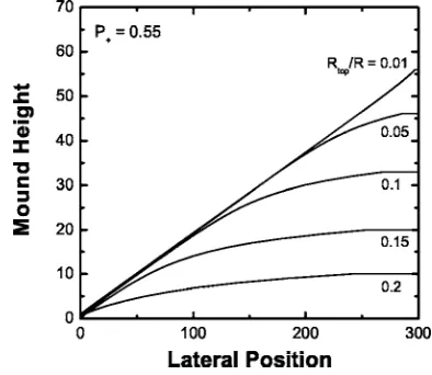
Next, we focus on characterization of selected mound shapes in the general case of inhibited interlayer transport. Figure 8 shows the selected mound shapes after a long-time evolution obtained from the analysis of the step dynamics model based on Eq.共2兲–共4兲withP₊= 0.55 andc= 1 / 2 for the various choices ofRtop. Clearly, mound shapes are strongly influenced by the prescription of nucleation: facile nucleation

共corresponding to small Rtop/R兲 produces narrow terraces and pointed mound peaks; inhibited mound nucleation共 cor-responding to largeRtop/R兲produces a significantly flattened mound peaks.

FIG. 6. Comparison of the evolution shape of a semi-infinte mound with DF共c= 1 / 2兲and without DF共c= 0兲at different cover-ages:共a兲 10,共b兲100, and共c兲500 ML. Here, we setP+= 0.55, and b= 1.

FIG. 7. Transient evolution and asymptotic selection of mound shapes for P₊= 1 and c= 1 / 2. Here, we setR= 100, R_top= 5, and b= 1. The number on the right side indicates the corresponding coverage for each mound shape.

For smaller Rtop/R, a region with well-defined selected slope, ms, emerges at least near the mound base.

Further-more, this slope corresponds to the value ofms⬁obtained in

the above analysis of semi-infinite mounds. For larger Rtop/R, the shape of the entire mound is impacted by top-layer nucleation, and no well-defined selected slope appears

共although the details of the shape are still strongly influenced by DF兲.

The above discussion considers only a deterministic pre-scription of nucleation. Thus, it is appropriate to ask what features are preserved for a more realistic stochastic prescrip-tion of nucleaprescrip-tion as described in Appendix A. With stochas-tic nucleation, evolution is no longer periodic. However, if one averages over many ML of deposition, one expects to find a well-defined mound shape with a smooth peak. Our analysis shows that using stochastic rather than deterministic nucleation produces at most a slight change in mound shape near the peak.

C. Net step attachment flux across the mound side

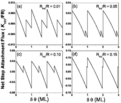
To further elucidate the selection of mound shapes, it is instructive to analyze the behavior of the net step attachment flux,Kˆtot, defined in Sec. II B. The long-time solution to Eqs. 共2兲,共3兲,共4兲for selected mound shapes in the model with DF is not time invariant. Rather, it is periodic in the reference frame of the growing film with period of 1 ML. Thus,Kˆ_tot also varies periodically as shown in Fig. 9. Just after nucle-ation of a top layer island, downhill contribution from the top terrace is almost zero as the width of this terrace is negli-gible. Thus,Kˆtot as determined from Eq.共5兲 withLn*= 0 is

expected to bepositive, since also the net uphill flux on other terraces should dominate the DF flux. As the top terrace grows, the downhill flux across it also grows and subse-quently dominates the uphill contributions. Thus, at some pointKˆ_totbecomes negative. In particular,Kˆ_totas determined from Eq. 共5兲 with Ln*=R_top is negative just before a new

layer is created. After the new top layer is created, it jumps by an amount 共1 +⌬兲共R_top/R兲 to recover its initial positive value decribed above.

There is also a jump within each period共in between top layer creation兲which corresponds to the disappearance of the bottom step. Just after the disappearance of this step, a broad bottom terrace is created upon which all depositing atoms are incorporated at the step to the right and create a significant uphill flux. Thus,Kˆtotjumps to a more positive value at this point.

Our key finding is that the mean value of Kˆtot averaged over 1 ML always vanishes 共when c⬎0兲 for deterministic nucleation. The impact of this condition on selected shape can be seen most clearly using Eq.共5兲. We consider only the typical case of mounds containing many steps where the maximum width of the bottom terrace is far smaller than the mound radius, so x₁/RⰆ1. Also, for selected shapes, the mound height␦h⬇bn* or b共n*− 1兲 共from valley to peak兲is roughly constant. Then, setting ␣=Ln*/R_top, the condition 具Kˆtot典= 0 implies that

共P+−P−兲− 2P+共Rtop/R兲具␣典− 2P+共c/b兲共␦h/R兲= 0, 共13兲 where 具␣典⬇1 / 2 denotes the time average of ␣. Eq. 共13兲 reflects a balance between the three main contributions to the total step attachment flux from the net uphill flux due to diffusion bias, and from the downhill fluxes due to diffusion across the top terrace and due to DF. It is immediately clear that, e.g., inhibited nucleation 共i.e., larger R_top/R兲 implies less high mounds. This condition has been successfully ap-plied to provide a boundary condition for continuum evolu-tion equaevolu-tions derived from coarse-graining of the step dy-namics equations.35

As an aside, a detailed analytic investigation of Kˆ_tot is presented in Appendix C for the extreme case whereRtop is sufficiently large that there are at most two steps during pe-riodic mound evolution. Finally, for stochastic nucleation, if one averages over many ML of deposition, one expects that the averagedKˆtotagain effectively vanishes. In this respect, the constraint on the net step attachment flux is preserved.

D. Evolution of a finite mound without DF

Step dynamics models without DF have been applied pre-viously to analyze mound evolution, both the steepening of individual wedding-cake-like mounds with no interlayer transport,31,32 _{and the evolution of quasiperiodic arrays of} mounds with a finite ES barrier.30 _{For the latter, mound} steepening with the development of deep grooves at mound valleys was observed for larger wavelengths. However, a transition to “steady-state” evolution was observed with de-creasing wavelength.30

Motivated by the latter, we consider the evolution of a single half-mound共representing a half period in a periodic array of mounds兲. Our analysis without DF implements de-terministic nucleation and considers behavior for fixed mound radius R but various choices of Rtop 共rather than changing the period of 2R兲. For sufficiently smallRtop/R, we find that a deep groove develops at the mound valley, analo-FIG. 9. Periodic variation of the net step attachment fluxKˆtot,

with coverage increment␦␪in the “steady-state” of model with DF

共c= 1 / 2兲. Behavior is shown for differentRtop.Rtop/R ⫽0.01共a兲, 0.05共b兲, 0.10 共c兲, and 0.15 共d兲, respectively. Here P₊= 0.52 and R= 1000.

MOUND SLOPE AND SHAPE SELECTION DURING¼ PHYSICAL REVIEW B73, 125434共2006兲

gous to behavior found in Ref. 30 for large wavelengths. However, ifR_top/Ris larger than a well-defined critical value rc then the mound evolves to a “stationary” shape. This

behavior is analogous to that found in Ref. 30 for short wavelengths. Note thatrcincreases with increasing diffusion

bias⌬.

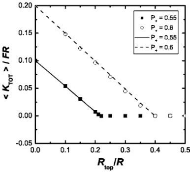
Here, we provide further insight into this transition by again considering the behavior of the net step attachment flux across the mound sideKˆtot. ForRtop/Rbelow the critical value rc corresponding to persistent roughening of the

mound, we find that the mean value具Kˆ_tot典, averaged over a period of 1 ML is strictly positive. 共This value depends somewhat on the time when the averaging is performed as the mound is continually steepening.兲In contrast,具Kˆ_tot典 van-ishes for steady-state evolution whenR_top/R exceedsrc. See

Fig. 10. Of course, for this model, there is no negative con-tribution toKtotfrom DF. Thus, the negative contribution to Ktotwhich is responsible for the vanishing of the mean value whenRtop/Rexceedsrccomes entirely from diffusion in the

downhill direction across the top terrace.

An approximate but reasonable estimate of 具Kˆtot典 and rc

comes from applying Eq.共5兲 with c= 0 and neglecting the term including x1. For smaller Rtop/R, we found from the analysis of step dynamics model that具Ln*典⬇0.42R_top. Then,

Eq.共5兲becomes

具Kˆ_tot典 ⬇⌬− 0.42共1 +⌬兲共R_top/R兲 共14兲 forRtop/R艋rcwithrc⬇2.38⌬/共1 +⌬兲. Finally, we note that

although a stationary shape is obtained forR_top/Rabove the critical value rc there is no tendency for slope selection 共without DF兲.

V. MOUND SHAPE AND SLOPE SELECTION IN PHENOMENOLOGICAL CONTINUUM TREATMENTS

Mound slope selection and subsequent evolution have been modeled extensively using phenomenological

con-tinuum theories共PCTs兲. In these PCTs for共1 + 1兲D, the evo-lution of a continuous film heighth共x,t兲at lateral positionx and timet, obeys1,8,12,30,43–47

⳵

⳵th共x,t兲=Fb− ⳵

⳵xJPCT共x,t兲. 共15兲 whereJPCTis a suitable mesoscale or coarse-grained lateral mass current which is proportional to F 共assuming no de-sorption and irreversible incorporation at step edges兲. It is an open and challenging problem to rigorously derive an ex-pression forJPCTstarting from an atomistic model. Typically, a phenomenological form is assumed whereJPCT is decom-posed asJPCT=Jup⫹JDF⫹JSB⫹Jrelax.

Here, J_up共m兲, which depends on the local slopem=_⳵⳵_xh, denotes the destabilizing net uphill current due to surface diffusion in the presence of inhibited interlayer transport.1,5 JDF共m兲denotes the downhill current due to DF. In the “sim-plest picture,”48 _{it is taken as the microscopic lateral} down-hill current associated with DF which is proportional to the step density, and thus to m.15,49–53 _{The term J}

SB produces up-down symmetry breaking, and Jrelax facilitates “relax-ation” near mound peaks and valleys.8,30 _{Shape selection in} the PCT corresponds to the vanishing of JPCT. For selected slopes on the straight sides of mounds共where bothJSBand J_relaxvanish兲, this corresponds to cancellation of theJ_upand JDF.

A simple estimate of the dominant behavior of JUP for broader terrace widthsL=b/兩m兩 significantly greater than c 共but still in the step flow regime兲 would suggest that J_up共m兲⬇Fb⌬L/ 2. A refined estimate from coarse-graining of step dynamics equations for local stair-case regions yields Jup共m兲⬇Fb⌬共L−c兲/ 2.35 In either case, assuming that JDF

⬀m leads to the result msPCT⬇共b/c兲

冑

apparent discrepancy with the predicted linear variation in the step dynamics model was noted previously,35but is mis-leading.

We now present a more detailed and precise analysis of the relevant microscopic lateral mass currents in our model

共based on the mean lateral distance travelled per depositing atom due to specific processes兲 for atoms depositing on a perfect staircase with terrace widthL. For DF, the fraction of atoms deposited in the step region is c/L, and mean lateral distance traveled by those atoms deposited isc/ 2. Thus, one has that

J_DF共m兲= −Fb共c/2兲共c/L兲= −Fc2_{m/2. 共16兲}

Next, consider the remaining fraction共L−c兲/Lof atoms de-posited on a terrace of widthLoutside the step edge region. Those attaching to the accending step共with probabilityP₊兲 travel an average distance of共L−c兲/ 2. Those attaching to the descending step共with probability P−兲travel an average dis-tancec+共L−c兲/ 2 =共L+c兲/ 2 accounting for the extra nondif-fusive motion across the step region. Thus, one has

Jup共m兲=Fb关P+共L−c兲/2 −P−共L+c兲/2兴共L−c兲/L

=Fb⌬共L−c兲/2 −Fbc共L−c兲/共2L兲. 共17兲

Setting Jup共m兲+JDF共m兲= 0 to obtain the selected slope FIG. 10. Dependence onRtop/Rof the mean value ofKˆtot

m=ms yields exactly the same result as obtained from the

step dynamics modeling, i.e., ms PCT_⬇共

b/c兲⌬, for small ⌬, crossing over tomsPCT=b/共2c兲, for⌬= 1.

There have been several simulation-based and analytic studies of slope selection for realistic astomistic models of homoepitaxial growth共effectively corresponding to a BCF-type rather than a constant choice of P±兲.15,23,49,51–53 These determined net lateral mass current,JPCT, and even separate contributions, based on the above microscopic definition, i.e., from the mean lateral distance traveled per deposited atom. These analyses of selected slope are thus consistent with that above.

There remains the challenge of developing reliable ex-pressions forJPCTin the evolution equation for a PCT. One strategy is to first obtain a “local” continuum evolution equa-tion by coarse graining of the step dynamics model over a single mound. This produces a JPCT without any DF or re-laxation terms, and which is nonvanishing over a single mound of selected shape.35_{This is not inconsistent with the} boundary conditions applied at the mound valley共which im-poses the selected slope兲 and at the peak. In any case, one could add or subtract a constant to JPCT without changing evolution. For the desired further-coarse grained evolution equation applicable for arrays of mounds, we are exploring the replacement of the boundary condition at the peak by effective relaxation term.35_{One must also reliably treat slope} selection and behavior near the mound valleys.

VI. DISCUSSION AND CONCLUSIONS

We have shown that refinement of conventional step dy-namics models incorporating downward funneling 共DF兲 deposition dynamics is a particularly effective tool for eluci-dation of mound shape and slope selection during unstable multilayer growth. Our analysis reveals how the incorpora-tion of DF共or other nonthermal downward transport mecha-nisms兲 leads to slope selection. A key effect of DF is to facilitate step annihilation at the mound valleys and thus to enhance the growth of the valley heights at the base of mounds.

A key concept in analysis of these step dynamics models is the net step attachment flux Ktot and the associated con-straint具Ktot典= 0, which controls selected mound shapes. It is natural to compare this picture with the steady-state condi-tion in PCT that the coarse-grained lateral mass current van-ishes, i.e., thatJ_PCT= 0. There is of course some similarity betweenKtot, or its local componentsKn andKDF, andJPCT. Indeed, we have shown consistency in the prediction of se-lected slopes from these two formulations. However, only K_tot is defined precisely and generally for the discrete step dynamics model, and only this quantity varies periodically alternating in sign 共with significant amplitude for larger Rtop/R兲.

Key concepts共e.g., related toKtot兲and analytic techniques 共e.g., for analysis of periodic solutions兲developed or utilized in this work have general applicability beyond the case of constantP±共for which we presented simulation results兲. As indicated in Sec. II, it is natural to consider a BCF-type choice ofP±as given in Eq.共5兲, which should be applicable

at least in the regime of broader terraces or smaller slopes. In our step dynamics model with DF for this choice, now a key parameter is the rescaled ES length lES=LES/c. Analysis of the selected slope for this model reveals a transition from smooth growth for lES⬍1 共where effectively ms= 0兲 to

mound formation with ms increasing linearly 共in lES兲 from zero forl_ES⬎1 and quickly saturating at a maximum value forlES=O共1兲. These observations have consequences for in-terpretation of experiments. For example, the small mound slopes observed in experimental and simulation-based stud-ies of the growth of Ag on Ag共100兲 at 300 K may not cor-respond to true selected slopes sincelESis likely significantly larger than unity.11_{Instead, the observed slopes may be} con-trolled by a relatively large value ofRtop/R for this system.

ACKNOWLEDGMENTS

This work was supported by NSF Grant No. CHE-0414378 and was performed at Ames Laboratory⫺USDOE which is operated by ISU under Contract No. W-7405-Eng-82. We acknowledge R.V. Kohn for insightful discussions which motivated this investigation. We also thank P. Politi for several valuable communications.

APPENDIX A: STOCHASTIC NUCLEATION

In the deterministic nucleation scheme used above, a new terrace or island is created on the top of a mound exactly when the radius of the current top terrace reaches a critical value ofRtop. In reality, the nucleation occurs for a distribu-tion of radii centered on such a “critical” value. Thus, a more realistic stochastic prescription of nucleation could be imple-mented based on a knowledge of this distribution.

Detailed analysis of the nucleation process on top of mounds indicates that the probability for no nucleation to have occurred is given by1,2

Pnonuc共t兲= exp

冋

冉

Risl共t兲 Rtop

冊

n

册

whereR_isl共t兲is the growing radius of the top island at a time t after its nucleation. The choice of the constant cn will be

described below. The value of the exponentndepends on the strength of the ES barrier. Adapting the existing analyses1_to 共1 + 1兲D, one can show that n= 5 forLESⰇLisl, andn= 6 for LESⰆLisl for the 共1 + 1兲D models described here. Different values are obtained for共2 + 1兲D models.54

Ifp_nucdtdescribes the probability for nucleation to occur between timestandt+dt, then it follows that

pnuc共t兲= d

dt共1 −Pnonuc兲, where

冕

⬁

pnuc共t兲dt= 1.

共A2兲 More usefully, ifp_nuc* dR_isl=p_nucdt describes the probabil-ity for nucleation to occur when the island radius is between RislandRisl+dRisl, it follows that

MOUND SLOPE AND SHAPE SELECTION DURING¼ PHYSICAL REVIEW B73, 125434共2006兲

p_nuc* 共Risl兲=ncn 共Risl兲n−1

共Rtop兲n

exp

冋

冉

Risl Rtop

冊

n

册

is determined from the constraint that 具Risl典=Rtop. Utilizing Eq.共A3兲, one obtains

共cn兲1/n=n

冕

⬁

dyyn_exp关−yn_{兴, 共A4兲}

so, e.g.,c5= 0.653 andc6= 0.637共wheren= 6 is used below兲. To implement stochastic nucleation, we determine a func-tion R_isl=R_isl共x兲 which recovers the correct distribution of island radii when x is selected as a uniformly distributed

random number on 关0,1兴. It thus follows that dx

=p_nuc* 共Risl兲dRisl, and consequently that

x=

冕

R_isl

p_nuc* 共R_isl兲dR_isl= 1 −P_nonuc. 共A5兲

In conclusion, one has that

Risl=Rtop

冋

ln关1 −x兴 cn

册

1/n

. 共A6兲

With this prescription, there is no upper limit on the range of R_isl. If R_top/R is significant, then some selected R_isl will likely exceed the mound radius,R. In this case, some refine-ment of the above probability distribution is required to im-pose an upper cuttoff of Risl⬍R. However, in the analysis below,Rtop/Ris sufficiently small that effectively all selected R_islare belowR.

In our numerical analysis of the evolution of a finite mound with stochastic nucleation, we use Eq.共A6兲 to gen-erate a sequence of values for Rtop which are used for the nucleation of successive top layers. We integrate Eqs. 共2兲,

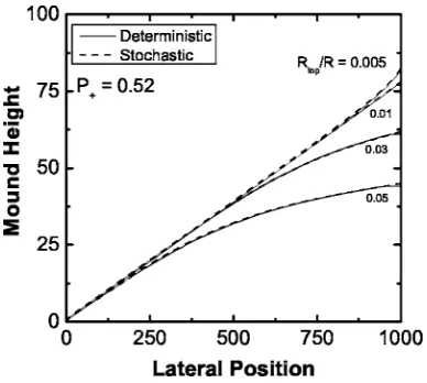
共3兲, and 共4兲 for some time to let the system evolve into a steady state, then average mound profiles obtained over many ML of deposition. Figure 11 compares such mound

profiles for the deterministic and stochastic nucleation schemes. The profiles are similar except very near the mound peak, which is flat for deterministic nucleation but smooth

共after averaging兲for stochastic nucleation.

APPENDIX B: PERIODIC EVOLUTION OF A SEMI-INFINITE MOUND:P₊= 1

Here, we determine the periodic solution for the evolution of a semi-infinite mound in the special case whereP₊= 1 and where the evolution equations adopt a simpler recursive form. Specifically, these equations become

dx1

d␪ = −x1−c,

dxn

d␪ = −共xn−xn−1兲, forn⬎1. 共B1兲

For the periodic solution just after the bottom step disap-pears, we assign the step positions asxn共␪= 0兲=xn

*_forn艌1. Then, the above equations can be solved recursively with these initial conditions and the additional requirement of ob-taining a periodic solution, i.e.,

x1共␪= 1兲= 0, x2共␪= 1兲=x1 *

, x3共␪= 1兲=x2 *

, . . . . 共B2兲

Integrating these equations leads to the recursion relations

x₁*=c共e− 1兲, 共B3兲

x₂*=共e− 1兲x*₁−c共e− 2兲, 共B4兲

xn*=共e− 1兲x1*−c共e− 2兲−

1 +xn−2 *

2! − ¯

− 1 +x1 *

共n− 1兲!, forn⬎2. 共B5兲

It is convenient to recast these equations for the terrace widths,L₀*=x₁*, and Ln

* =xn+1

* −xn

*

forn⬎1, as

L₀*=c共e− 1兲, 共B6兲

L₁*=共e− 1兲L₀*−c, 共B7兲

Ln*=共e− 1兲Ln*−1− Ln−2

*

2! − ¯−

L₁* 共n− 1兲!

−ce

n!, forn⬎2. 共B8兲

Solving these equations yields

L₀*=c共e− 1兲= 1.71828c, 共B9兲

L₁*=c共e2_{− 2e兲= 1.95249c, 共B10兲}

L₂*=c共e3− 3e2− 3e/2兲= 1.99579c, 共B11兲

L₃*=c共e4− 4e3+ 4e2− 2e/3兲= 2.00003c, . . . 共B12兲 FIG. 11. Comparison of the deterministic and stochastic

More direct analysis of the limiting behavior, as n→⬁, which is of primary interest, comes from utilizing a suitable ztransform xˆ共z,␪兲=兺n⬁=1z

n

xn共␪兲. Applying this transform to

the evolution equations yields a simple ordinary differential equation forxˆ共z,␪兲 which can be solved to obtain

xˆ共z,␪兲=xˆ共z,0兲e−共1−z兲␪− z 1 −z关1 −e

−共1−z_兲␪_兴

, for 0⬍␪⬍1.

共B13兲 Imposition of the boundary condition for a periodic solution requires that

xˆ共z,1兲=zxˆ共z,0兲. 共B14兲

Substituting into Eq.共B13兲finally yields the result

xˆ共z,0兲= − z 1 −z

exp关1 −z兴− 1 zexp关1 −z兴− 1⬃

2c

共1 −z兲2, as z→1. 共B15兲 Since xn

*_⬃

const+nL_⬁ for large n, it follows that xˆ共z, 0兲

⬃L_⬁/共1 −z兲2 as z→1, so L_⬁= 2c. In conclusion, we obtain the exact resultms⬁=b/共2c兲 forP+= 1.

Finally, we note that forP+⬍1, a recursive analysis is not possible. However, application of a suitable modified trans-form to the evolution equations should allow an exact treat-ment.

APPENDIX C: EXACT ANALYSIS OF A THREE-LEVEL SYSTEM

To further elucidate the periodic evolution of finite mounds共either with or without DF兲, it is natural to consider the “extreme” case corresponding to large Rtop⬍R where there are at most two steps. In this case, there are at most three levels of terraces, so the evolution corresponds to a so-called three-level system. Below, we setR_top=R−xc, and

assume constantP_±.

We consider an “initial” configuration for periodic evolu-tion as corresponding to the time just after nucleaevolu-tion of the second upper island of step. See Fig. 12共a兲. Then, one has thatx₁共␪= 0兲=xc, and x2共␪= 0兲=R.

There are two distinct stages of the mound evolution. In the first stage for 0⬍␪⬍␪*共⬍1兲, say, beforex1reaches zero 共at␪=␪*兲, the mound has two steps as shown in Fig. 12共b兲. The evolution of these two steps is described by

dx1

d␪ = −x1−P−共x2−x1兲−c, 共C1兲

dx2

d␪ = −P+共x2−x1−c兲−共1 −x2兲. 共C2兲

It is more convenient to transform these equations intro-ducing new dependent variables x₂−x₁ and x₂+x₁, noting that d共x₂+x₁兲/d␪= −R.共There is a natural generalization of this latter relation for mounds with any number of steps.兲 Integrating these equations for␪⬍␪*, one obtains

x2+x1=xc+共1 −␪兲R, 共C3兲

x2−x1=

冉

⌬+

R

⌬2+c 1 +⌬

⌬

冊

⌬ .

共C4兲

At ␪=␪* when x1 vanishes, these two quantities become equal, which imposes a key constraint on␪* _{utilized below.} Finally, we note that in this first stage, the net step attach-ment flux is given by

K_tot1 /F=x1+x2− 1 +⌬共x2−x1−c兲−c 共C5兲

and can thus be calculated exactly from the above results. Figure 12共c兲illustrates the second stage of mound evolution where there is only one step, starting when x1 vanishes at ␪=␪* and ending when x2=xc at ␪= 1. In this regime, the

evolution of step 2 is trivially given by

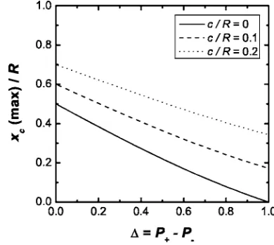
FIG. 13. The behavior of x_c共max兲 with ⌬ in the three-level system for the different choices ofc/R.

FIG. 12. Schematic of the evolution of a mound with at most two steps:共a兲initial state,共b兲first stage beforex₁reaches zero,共c兲 second stage where there is only one step following the disappear-ance of the original bottom step.

MOUND SLOPE AND SHAPE SELECTION DURING¼ PHYSICAL REVIEW B73, 125434共2006兲

dx2

d␪ = −R, 共C6兲

sox2=xc+共1 −␪兲R. The net step attachment flux in the

sec-ond stage is given by

K_tot2 /F= 2x2−R, 共C7兲

and can thus be readily calculated using Eq.共C6兲.

Next, we investigate the average value具K_tot典, ofK_totover a period of 1 ML,

冓

冔

冕

␪*

d␪K_tot1 /F+

冕

␪* 1

d␪K_tot2 /F

= −

冉

⌬ +

R

⌬2+

2c共1 +⌬兲

⌬

冊

* 兲

−共R−xc兲e−⌬␪ *

+␪ *_R

⌬ + 2xc−␪*R. 共C8兲

Given the constraint on␪*_{mentioned above, it follows that} 具K_tot典 ⫽ 0. This result holds for the general c 共including c= 0 corresponding to no DF兲.

Finally, we have noted that the above three-level system picture of periodic evolution applies only for sufficiently largeRtop共or sufficiently smallxc兲. The specific condition for

the maximum possible valuexc共max兲 of xccomes from the

constraint on ␪* _{mentioned above, after setting␪}*_{= 1.} Spe-cifically, one obtains

xc共max兲=

共

⌬2+c 1+⌬

⌬

兲

R

⌬

1 −1−_⌬e−⌬+e−⌬ . 共C9兲 For ⌬= 0, one has xc共max兲=R/ 2 +c. For ⌬= 1, one has

xc共max兲=c共e− 1兲. The behavior of xc共max兲 for the general

case is shown in Fig. 13.

1_{T. Michely and J. Krug, Islands, Mounds and Atoms: Patterns} and Processes in Crystal Growth Far from Equilibrium

共Springer, Berlin, 2004兲.

2_{J. W. Evans, P. A. Thiel, and M. C. Bartelt, Surf. Sci. Rep.共to be}

published, 2006兲.

3_{G. Ehrlich and F. G. Hudda, J. Chem. Phys. 44, 1039共1966兲.} 4_{R. L. Schwoebel and E. J. Shipsey, J. Appl. Phys. 37, 3682}

共1966兲.

5_{J. Villain, J. Phys. I 1, 19共1991兲.}

6_{A. Pimpinelli and J. Villain, Physics of Crystal Growth共}

Cam-bridge University Press, CamCam-bridge, 1998兲.

7_{H.-J. Ernst, F. Fabre, R. Folkerts, and J. Lapujoulade, Phys. Rev.}

Lett. 72, 112共1994兲.

8_{J. A. Stroscio, D. T. Pierce, M. D. Stiles, A. Zangwill, and L. M.}

Sander, Phys. Rev. Lett. 75, 4246共1995兲.

9_{J.-K. Zuo and J. F. Wendelken, Phys. Rev. Lett. 78, 2791共1997兲.} 10_{C. R. Stoldt, K. J. Caspersen, M. C. Bartelt, C. J. Jenks, J. W.}

Evans, and P. A. Thiel, Phys. Rev. Lett. 85, 800共2000兲. 11_{K. J. Caspersen, A. R. Layson, C. R. Stoldt, V. Fournee, P. A.}

Thiel, and J. W. Evans, Phys. Rev. B 65, 193407共2002兲. 12_{M. Siegert and M. Plischke, Phys. Rev. Lett. 73, 1517共1994兲.} 13_{M. C. Bartelt and J. W. Evans, Phys. Rev. Lett. 75, 4250共1995兲.} 14_{P. Smilauer and D. D. Vvedensky, Phys. Rev. B 52, 14263}

共1995兲.

15_{J. G. Amar and F. Family, Phys. Rev. B 54, 14742共1996兲.} 16_{J. W. Evans, D. E. Sanders, P. A. Thiel, and A. E. DePristo, Phys.}

Rev. B 41, 5410共1990兲.

17_{J. W. Evans, Phys. Rev. B 43, 3897共1991兲.}

18_{H. C. Kang and J. W. Evans, Surf. Sci. 271, 321共1992兲.} 19_{D. E. Sanders and J. W. Evans, inThe Structure of Surfaces III,}

edited by S. Y. Tong, M. A. Van Hove, K. Takayanagi, and X. D. Xie共Springer, Berlin, 1991兲, pp. 38.

20_{D. E. Sanders, D. M. Halstead, and A. E. DePristo, J. Vac. Sci.}

Technol. A 10, 1986共1992兲.

21_{J. Yu and J. G. Amar, Phys. Rev. Lett. 89, 286103共2002兲.} 22_{J. Yu and J. G. Amar, Phys. Rev. B 69, 045426共2004兲.}

23_{M. Siegert and M. Plischke, Phys. Rev. E 53, 307共1996兲.} 24_{J. G. Amar, Phys. Rev. B 60, R11317共1999兲.}

25_{H.-C Jeong and E. D. Williams, Surf. Sci. Rep. 34, 171共1999兲.} 26_{W. K. Burton, N. Cabrera, and F. Frank, Philos. Trans. R. Soc.}

London 243, 299共1951兲.

27_{N. Israeli and D. Kandel, Phys. Rev. Lett. 80, 3300共1998兲; Phys.}

Rev. B 60, 5946共1999兲; 62, 13707共2000兲.

28_{D. Margetis, M. J. Aziz, and H. A. Stone, Phys. Rev. B 69,}

041404共2004兲; 71, 165432共2005兲.

29_{I. Elkinani and J. Villain, J. Phys. I 4, 949共1994兲.} 30_{P. Politi and J. Villain, Phys. Rev. B 54, 5114共1996兲.} 31_{J. Krug, J. Stat. Phys. 87, 505共1997兲.}

32_{J. Krug, Physica A 313, 47共2002兲.}

33_{W. E and N. K. Yip, J. Stat. Phys. 104, 221共2001兲.}

34_{R. V. Kohn, T. S. Lo, and N. K. Yip, inStatistical Mechanical}

Modeling in Materials Science, edited by M. C. Bartelt et al., MRS Symposia Proceedings No. 701共Materials Research Soci-ety, Warrendale, PA, 2002兲, p. T1.7.

35_{Maozhi Li and J. W. Evans, Phys. Rev. Lett. 95, 256101共2005兲;}

Phys. Rev. Lett. 96, 079902共E兲 共2006兲.

36_{J. Tersoff, A. W. Denier van der Gon, and R. M. Tromp, Phys.}

Rev. Lett. 72, 266共1994兲.

37_{J. Rottler and P. Maass, Phys. Rev. Lett. 83, 3490共1999兲.} 38_{J. Krug, P. Politi, and T. Michely, Phys. Rev. B 61, 14037共2000兲.} 39_{C. Castellano and P. Politi, Phys. Rev. Lett. 87, 056102共2001兲.} 40_{Note that another viable implementation of top layer nucleation}

would set x_n*₊₁=R−c so L_n*=c at the time of nucleation, t=t_n⬘*₊₁. Behavior will not vary significantly from that for the choicexn*+1=RsoLn*= 0 used in this study. Note that the last two terms in Eq.共4兲can be contracted as −FL_n*, which varies smoothly in either case.

41_{The three-step approximation yielded ill-behaved 共}

complex-valued兲solutions, and thus cannot be used.

42_{P. Politi, cond-mat/0601655, C. R. Phys.共to be published兲.}

43_{M. Siegert, Phys. Rev. Lett. 81, 5481共1998兲.}

Lett. 89, 266104共2002兲.

45_{A. Levandovsky and L. Golubovic, Phys. Rev. B 69, R241402}

共2004兲.

46_{R. V. Kohn and X. Yan, Commun. Pure Appl. Math. 56, 1549}

共2003兲.

47_{B. Li and J.-G. Liu, Eur. J. Appl. Math. 14, 713共2003兲.} 48_{P. Politi, G. Grenet, A. Marty, A. Ponchet, and J. Villain, Phys.}

Rep. 324, 271共2000兲.

49_{J. G. Amar and F. Family, Phys. Rev. B 54, 14 071共1996兲.}

50_{J. G. Amar and F. Family, Phys. Rev. Lett. 77, 4584共1996兲.} 51_{V. Borovikov and J. G. Amar, Phys. Rev. B 72, 085460共2005兲.} 52_{M. C. Bartelt and J. W. Evans, inEvolution of Epitaxial Structure}

and Morphology, edited by Andrew Zangwillet al., MRS Sym-posia Proceedings No. 399共Materials Research Society, Warren-dale, PA, 1996兲, p. 89.

53_{M. C. Bartelt and J. W. Evans, Surf. Sci. 423, 189共1999兲.} 54_{In 共2 + 1兲D, one obtains n= 7 for L}

ESⰇLisl, and n= 8 for LES

ⰆL_isl.

MOUND SLOPE AND SHAPE SELECTION DURING¼ PHYSICAL REVIEW B73, 125434共2006兲