SRef-ID: 1432-0576/ag/2005-23-2081 © European Geosciences Union 2005
Annales
Geophysicae
The effect of
E
-region wave heating on electrodynamical structures
J.-M. A. No¨el1, J.-P. St.-Maurice2, and P.-L. Blelly3
1Department of Physics, Royal Military College of Canada, Kingston, Ontario, Canada
2Department of Physics and Engineering Physics, The University of Saskatchewan, Saskatoon, Saskatchewan, Canada 3Laboratoire de Physique et Chimie de l’Environnement, Orl´eans, France
Received: 16 September 2004 – Revised: 22 March 2005 – Accepted: 20 June 2005 – Published: 15 September 2005
Abstract. We show that heating by large amplitudeE-region
plasma waves at high latitudes can at times substantially en-hance the electro-dynamical response of the ionosphere. This is made manifest through an increase in parallel current den-sities and parallel electric fields generated at the edge of arcs in theEand lowerF-region of the ionosphere, in response to sharp cutoffs in precipitation with an otherwise uniform differential energy flux. The enhancement is rooted in a re-duction in electron recombination that occurs in response to higher electron temperatures triggered by the generation of strong electric fields near the edge of the arc. The reduced recombination rate, in turn, leads to enhanced conductivity gradients near the edge of the arc, which, in turn, drives more intense parallel currents and stronger local electric fields.
Keywords. Ionosphere (Electric fields and curents; Plasma
temperature and density) – Space plasma physics (Numerical simulation studies)
1 Introduction
St.-Maurice et al. (1996) have argued that a host of unusual phenomena sometimes seen near auroral arcs can be ex-plained in terms of electro-dynamical phenomena in the pres-ence of unusual precipitation patterns. The unusual observa-tions include very large shears in the horizontal plasma drifts near certain arcs, large magnetic perturbations detected on board satellites or rockets, as well as the observation by in-coherent scatter radars of large amplitude ion-acoustic waves along the geomagnetic field line. No¨el et al. (2000) have therefore studied in some detail the electrodynamics of two-dimensional auroral arcs which, instead of being associated with inverted V precipitation patterns, would be triggered by a flat precipitation pattern coupled with a sharp horizon-tal/latitudinal cutoff (200 m). They showed that the intro-duction of this kind of precipitation pattern did not lead to
Correspondence to: J.-M. A. No¨el
the usual short-circuiting of the perpendicular electric field and weak parallel current densities associated with “normal” inverted-V arcs. Instead, they obtained thermal parallel cur-rent densities that became extremely large at the edges of the arc while the perpendicular electric field was perturbed only near the edges, with very little change short-circuiting ef-fects near the center of the arc. In addition, the perpendicular electric field became larger just outside the arc and weaker just inside the arc. To be more precise, No¨el et al. (2000) showed that, consistent with back-of-the-envelope calcula-tions for such situacalcula-tions, parallel current densities of several 100µA/m2could be carried by thermal electrons, provided that a sufficiently large DC electric field or a sufficiently sharp drop in precipitation flux was used. With 200-m hori-zontal cut-off scales in precipitation, ambient perpendicular electric fields of the order of 50 mV/m or more were required. The No¨el et al. (2000) calculations included a state-of-the-art description of the chemistry and of the transport and electron cascading processes along the geomagnetic field lines. A coupling of the various field lines was introduced by imposing the condition that the currents in the system be divergence-free. However, one process that was not included in the original calculations was the repeated observed heat-ing of electrons atE-region heights in the presence of strong electric fields. In this paper we have now included this heat-ing. We are able to show that the additional electron heating has a surprisingly strong effect on the results, in that it actu-ally increases further the parallel electric fields and currents at the edges of the kinds of arcs that trigger strong parallel current responses at their edges.
Since our work introduces the contribution of electron heating to the electro-dynamical ionospheric feedback, for the first time, we feel that a brief overview of the subject should be in order.
invoked to connect the irregularities to electron heating. The first has been associated with anomalous perpendicular dif-fusion, in effect, enhanced broadband perpendicular fields (Robinson, 1986; St.-Maurice, 1987). The second has in-voked wave parallel fields, since it is well known that the irregularities can be a few degrees off perpendicularity to the magnetic field under strong DC electric field conditions (St.-Maurice and Laher, 1985; St.-(St.-Maurice, 1990b; Milikh and Dimant, 2002; Dimant and Milikh, 2003; Milikh and Dimant, 2003).
In our work it is important to have a quantitative descrip-tion of the electron heating effects that is both easy to pro-gram and that has been tested against observations. Two such descriptions currently exist, one for each of the proposed wave mechanisms. Both descriptions have been claimed to work well. The one from Robinson (1986), which relies on anomalous diffusion, is particularly simple to use and it has been tested repeatedly and shown to work well. However, another expression has recently been proposed by Dimant and Milikh (2003), using the parallel wave heating mecha-nism. These latter authors have also claimed that their for-mula works, though on the face of it, it certainly looks quite different, as we show below. Particularly in the large electric field regime that interests us here, a regime that has not been tested as thoroughly, there may be some differences between the two prescriptions.
While the Robinson (1986) formula has been tested more thoroughly and is simpler to use, there are physical reasons why one would come to favor the more complicated and less tested Dimant and Milikh (2003) expressions. For instance, the Robinson (1986) saturation mechanism involves a diffu-sive process which is at right angles to the one required to saturate the waves (St.-Maurice, 1990a). Another troubling point out is that St.-Maurice and Hamza (2001) have pointed in their work on intermittency that the electric field inside the irregularities is actually smaller than the ambient field: the presence of the structures should, after all, act to short out electric fields within the structures themselves, not en-hance them. This implies that the total heating rate should go down, not up, in the presence of perfectly field-aligned structures, since the field in such structures is systematically less than the ambient field. This point is often overlooked in linear theories, so that when the linear results are used in quasi-linear expressions they lead to erroneous results.
In the end, we have simply chosen to study the effect of electron heating using the two separate prescriptions. The Robinson (1986) prescription has the virtue of having been repeatedly tested and shown to do well. However, the less tested Dimant and Milikh (2003) prescription has a different physics that may well be working better in the end. There-fore, with claims from both sides that the formulae agree well with observations, we can provide with our work a test of whether or not this is the case, and whether or not apparently small differences can have important consequences.
Given the background described above, we will, in the present paper, focus once again on the modelling of elon-gated auroral structures created by uniform particle
precipi-tation with sharp cut-offs in their latitudinal pattern. We will once again add the presence of large ambient electric fields, so as to trigger large parallel current densities on the edge of the structures. The goal will simply be to quantify and un-derstand the effects of electron heating by Farley-Buneman waves, first on the energetics, and then on the composition and the electrodynamics.
The rest of our paper unfolds as follows: in Sect. 2 we describe our electrodynamic model, as well as the modifi-cations that were made to the transport model, so as to take into account the wave-induced electron heating. In Sect. 3 we present results from our model for the cases without anoma-lous electron wave heating, with wave heating using Robin-son’s expression and finally, with wave heating using Dimant and Milikh’s expression. We end with a summary and con-clusion in Sect. 4.
2 The Model
2.1 Basic description
A complete description of the basic model used in our elec-trodynamical calculation, as well as the numerical technique, can be found in No¨el et al. (2000). We only briefly review the procedure here.
The model is two-dimensional in x (north–south) and z (magnetic field) directions. The east–west, ory-derivatives, are neglected under the assumption of an elongated east-west precipitation pattern and arc. Aside from this, the model is made of two distinct parts. The first part consists of the comprehensive time-dependent transport TRANSCAR model, which has been used as a basis for many studies over the years. The second part of the model is an electrodynam-ical model which we call ELECTRO. Our main focus here will be on the equations that we modified in order to add an electronE-region wave heating term.
A complete description of TRANSCAR is provided in Blelly et al. (1996). In short, TRANSCAR is a one-dimensional program that models the terrestrial ionosphere in the altitude range 100–3000 km, along the geomagnetic field. It itself consists of two parts. The first part of TRAN-SCAR is a fluid description of the ionosphere and is based on the 8-moment transport formulation (Blelly and Schunk, 1993). The model includes six thermal ion species (O+,
H+, N+, NO+, N+
2 and O
+
kinetic model provides the ion production rates and electron heating source for the fluid model.
In Fig. 1, we present the precipitating electron spectral flux that was used in simulations for both the present study and the one published by No¨el et al. (2000). The total particle flux is 2.3×10¹³m−2s−1and corresponds to an energy flux of 6 mW m−2into the ionosphere. This spectral flux was cho-sen because the energy of the precipitating electrons was high enough to penetrate deep into theE-region and to ionize it. The shape of the spectral flux is in agreement with those that can be found in a number of references (e.g., Rees, 1989; Blelly et al., 1996).
The electrodynamical part of the model, ELECTRO, is based on an approach first suggested by St.-Maurice et al. (1996) and No¨el et al. (2000). It assumes that the current density is divergence-free, which is not a problem for the time and spatial scales of interest,
∇ ·J =0. (1)
This equation means that for the temporal and spatial scales of interest, the perturbed electric fields and resulting currents are adjusting instantaneously to any temporal change in con-ductivity or precipitation input.
An important point about the procedure used to solve the problem at hand is that we do not make any assumption about the magnitude of the “perturbed” electric fields. We simply separate the current densityJ into three parts and carry on with the calculations. The first part is made up of a source term due to precipitation, Jps, i.e. it describes the currents
carried by precipitating fluxes of energetic electrons. The behavior of that current source is modelled through the ki-netic part of TRANSCAR mentioned earlier. The second source term is related to the presence, prior to the introduc-tion of precipitaintroduc-tion, of a uniform background electric field to which computed conductivity gradients will be added. Fi-nally, we have the most important contribution in our work by far, namely, a “thermal response term”, Jt h, which
de-pends on the perturbed electric field or potential, as well on the conductivities.
The last two current density terms are described with the use of a simple Ohm’s law, namely, from the equation
J =σ·E, (2)
where σ is the classical conductivity tensor, and E is the electric field. The conductivity tensor is, in turn, given by
σ =
σP σH 0
−σH σP 0
0 0 σk
, (3)
whereσP,σH andσkare the usual Pedersen, Hall and
paral-lel conductivities, respectively.
As stated above, we have divided the electric field into two parts, namely, E=E0−∇φ, where E0 is a constant back-ground electric field andφis the electrostatic potential of the
102 103 104
102
103
104
105
106
particle flux : 2.3 * 10**13 m−2.s−1
energy flux : 5.96 mW.m−2
mean energy : 1.62 keV
Electron Flux [ eV
−
1.cm
−
2.s
−
1.sr
−
1]
[image:3.595.308.546.64.259.2]Energy [ eV] Electron Precipitation Spectral Flux
Fig. 1. Spectral flux of the precipitating electrons.
disturbed field caused by the creation of the auroral arc intro-duced by the electron precipitation at timet=0. As a result Eq. (1) becomes
∇ ·J = ∇ ·(σ·E0)+ ∇ ·Jps − ∇ ·(σ· ∇φ)=0. (4)
Since we considerE0to be constant and uniform and since σ is computed using TRANSCAR’s output, the first term on the right-hand-side of Eq. (4) can be viewed as another source term by ELECTRO. Given that the ambient electric fieldE0is assumed to be perpendicular to the geomagnetic field and that we assume they-direction to be derivative-free, we rewrite this first term as
∇ ·(σ·E0)=Ex0∂σP (x, z)
∂x +E
0
y
∂σH(x, z)
∂x , (5)
where the terms ∂σP ,H/∂x are the horizontal north-south
gradients in the Pedersen/Hall conductivities that are created at the edge of the precipitating region. For simplicity we limit ourselves for now to the case whereEy0is negligibly small.
−100 −9 −8 −7 −6 −5 −4 −3 −2 −1 0 0.2
0.4 0.6 0.8 1 1.2
Horizontal Position (km)
Precipitation Factor, f(x)
[image:4.595.48.286.63.255.2]Maximum Precipitation Minimum Precipitation
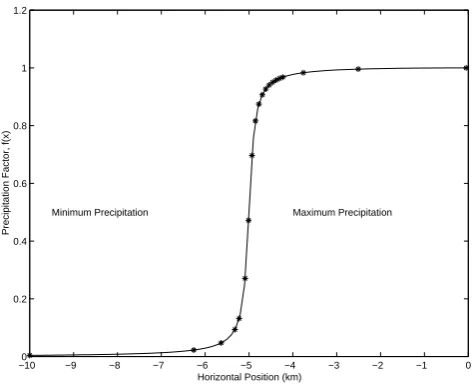
Fig. 2. Figure showing the field lines used in the computation.
one order of magnitude too small a scale). Even with this op-timistic number, however, we only obtain 10−9A/m3, which is totally negligible by comparison to the first term. We ver-ified, through numerical runs made with and without it, that the precipitating currents indeed played no role through the presence of the second term on the right-hand side of Eq. (4). Therefore, in order to speed up the calculations, we have, af-ter these tests, simply discarded the af-term in question.
After neglecting the divergence in precipitating currents, and with the help of Eq. (5) we have rewritten Eq. (4) in the form
∂ ∂x
σP(x, z)
∂φ (x, z) ∂x
+ ∂
∂z
σk(x, z)
∂φ (x, z) ∂z
≈Ex0∂σP(x, z)
∂x , (6)
whereφ (x, z)is the electric potential introduced by the hor-izontal and “vertical” gradients in conductivities triggered by the precipitation that we introduce at timet=0.
For the conductivities, we use standard expressions that may be found in a number of references. These expressions are presented in detail in No¨el et al. (2000) and will not be repeated here. The only point to stress is that the conduc-tivities are not only functions of altitudezbut also functions of the latitudinal positionx, through changes in the plasma density that are introduced by the arc. From Eq. (6) we can then see that a structuring of the conductivities has to cause a structuring of the electric potential and, therefore, of the associated electric fields and current densities.
Once the electric fields and current densities as a function of position have been determined using ELECTRO, they are fed into the transport equations (TRANSCAR) to determine the new concentrations, temperatures, field-aligned veloci-ties and field-aligned heat flows. The resulting densiveloci-ties and temperatures are then returned to ELECTRO to compute the
changes in the conductivities and the new electric potential via Eq. (6) and the associated electric fields and current den-sities. The iterations continue in this way as time advances.
Figure 2 describes the function used to model the latitu-dinal distribution of the electron precipitation in our sim-ulation. The asterisks indicate the field lines simulated by TRANSCAR. Note that we concentrate the field lines in the region of the maximum gradients in the precipitation profile. This is necessary in order to model the sharp precipitation gradients with adequate coverage.
A summary of the physics that we study with our model unfolds as follows: At first, precipitation creates regions of enhanced electron densities that modify the conductivities. Since we have a region of enhanced conductivities there must exist a gradient in the conductivities, concentrated, in this case, near the edge of the structure. This conductivity gra-dient rearranges the electric potential and associated electric field around the edge of the structure. The modified field, de-pending on the sign of its perturbation, can locally enhance or decrease the Joule heating rate of ions, as well as elec-trons. In the latter case the frictional heating rate is effec-tively increased by close to one order of magnitude in the 100 to 120 km region, owing to the heating by theE-region plasma irregularities discussed in the Introduction. It is the effect of this additional electron heating term that we wish to examine in detail in the present work in light of our 2-D elec-trodynamical model. Simply put, elevated electron temper-atures reduce the recombination rate (e.g., Sheehan and St.-Maurice, 2004). This means enhanced densities and there-fore higher conductivities in the hotter regions. This, in turn, modifies the conductivity gradients, and through them, the parallel currents and the ambient electric fields. We show below that the feedback can be positive and substantial for the steep precipitation cutoffs under study here, and we de-scribe how the feedback operates, by studying the results of our calculations with and without the electron wave heating term.
2.2 Modifications brought to the standard TRANSCAR model
The equations used in the fluid formulation of the transport part of TRANSCAR may be found in Blelly and Schunk (1993) and Blelly et al. (1996). We only discuss here our modifications to the electron energy equation in response to E-region wave heating of electrons.
The Joule heating rate contribution from species s nor-mally used by TRANSCAR is given by the standard expres-sion (e.g., Schunk and Nagy, 2000)
QsE= nse
2
sνsE⊥2
ms νs2+2s
, (7)
whereE⊥is the perpendicular convective electric field
am-plitude measured from the neutral frame of reference, B is the magnetic field strength, s=esB/ms is the
s, νs=Ptmsνst/(ms+mt) is the momentum transfer
fre-quency between ionized speciessand speciest,ms andmt
are the masses of species s andt, respectively, and QsE is the heating rate of speciessdue to the perpendicular electric field.
2.2.1 Robinson’s expression for the electron heating rate In TRANSCAR, the classical heating rate for the electrons has been modified to include the electron heating rate by plasma waves. For a first set of calculations, we used the expressions developed by Robinson (1986). According to Robinson’s prescription, the wave heating rate is described as follows: forvd<cs we use the classical heating rate for
the electrons which reads Qe =Qclassical=
nee2νeE⊥2
me νe2+2e
. (8)
However, ifvd>cs, it can easily be shown that Robinson’s
heating rate is given instead by the expression Qe =Qclassical+
ieme
νi
(vd−cs)3
cs
, (9)
wherevd is the magnitude of theE×Bdrift and the electric
field, as always, is measured in the neutral frame of refer-ence. Also,cs=
√
kb(Ti+Te) /mi is the ion-acoustic speed,
wherekbis the Boltzmann constant,TiandTeare the ion and
electron temperatures, respectively, andmiis the average ion
mass.
2.2.2 Dimant and Milikh’s heating rate
More complicated expressions, but also probably more phys-ically correct ones, were recently derived by Dimant and Mi-likh (2003), to describe the heating of electrons by wave par-allel electric fields. Given the complexity of the problem, the authors had to use a heuristic model of the saturated turbulent electric field, but ended up, nevertheless, with expressions that seemed to reproduce the observations well. This partic-ular wave heating model leads to a temperature expression described by
1Te
T0 = 4κi2νin
3δenνen
EC2
E002
(
1+ψ⊥
1+κi2
!
(EC−ET hr)3
EC2ET hr
+ψ⊥ "
1+
1−ET hr
EC
2#)
, (10)
whereδenνenis electron energy loss rate, while1Te=Te−T0
is the temperature increment and Te is the actual electron
temperature whileT0 is, in effect, the neutral temperature. The amplitude of the DC electric field is given byEC and
the dimensionless parametersψ⊥andκi are defined by
ψ⊥=
νenνin
ei
(11) and
κi =
i
νin
, (12)
whereiis the gyrofrequency of the ions andνen,νinare the
collision frequencies with the neutrals. The threshold electric field,ET hr, is given by
ET hr =(1+ψ⊥)
1+κi2 1−κi2
!1/2
E0,
where
E0=csB0=
s
kB(Te+Ti)
mi
B0,
where B0is the geomagnetic field amplitude andmi is the
average ion mass. Finally,
E00= s
2kBT0 mi
B0 (13)
is the Farley-Buneman threshold electric field in the undis-turbed ionosphere.
We notice thatψ⊥depends onTethrough the momentum
transfer collision frequencyνen. If we consider that the
neu-tral atmosphere consists mainly of N2, O2 and O, we have from Table 4.6 of Schunk and Nagy (2000) the following expressions for the electron-neutral momentum transfer col-lision frequencies, in s−1:
eand N2:
ν (e,N2)=2.33×10⁻¹¹n (N2)1−1.21×10⁻⁴Te
Te; (14)
eand O2:
ν (e,O2)=1.82×10⁻¹⁰n (O2)
1+3.6×10⁻²pTe
p
Te
; (15)
eand O:
ν (e,O)=8.9×10⁻¹¹n (O)1+1.57×10⁻⁴Te
p
Te. (16)
In these expressions, the densities are in cm−3and the tem-peratures in K. Clearly, ifTeis structured, then so isψ⊥and
consequentlyET hr. Furthermore, ifECis horizontally
struc-tured,Tehas to reflect that structure as well.
3 Results
−7 −6 −5 −4 −3 100
150 200 250 300 350 400
Altitude ( km )
Electron Density
m−3
0.5 1 1.5 2 2.5 3 x 10¹¹
−7 −6 −5 −4 −3 100
150 200 250 300 350 400
Altitude ( km )
O+ Density
m−3 5 6 7 8 9 10 x 1010
−7 −6 −5 −4 −3 100
150 200 250 300 350 400
Altitude ( km )
Electron Temperature
K1000 2000 3000 4000 5000 6000
−7 −6 −5 −4 −3 100
150 200 250 300 350 400
Horizontal Position (km)
Altitude ( km )
NO+ Density
m−3
0.5 1 1.5 2 2.5 3 x 10¹¹
−7 −6 −5 −4 −3 100
150 200 250 300 350 400
Altitude ( km )
O+ Temperature
K1000 2000 3000 4000 5000 6000
−7 −6 −5 −4 −3 100
150 200 250 300 350 400
Horizontal Position ( km ) NO+ Temperature
K1000 2000 3000 4000 5000 6000
Fig. 3. TRANSCAR output in the absence ofE-region electron heating by plasma waves and with the precipitation flux given in Fig. 1.
We note that the effects of theE-region electron heating on the energetics, composition, electrodynamics and the feed-backs between them, would simply not be taking place with-out a large magnitude for the electric field, since the heating only becomes considerable once the electric field exceeds 50 mV/m. We have therefore limited our study here to the 100 mV/m case and to the sharp precipitation cutoffs already considered by No¨el et al. (2000), since this is the kind of physical situation for which the E-region electron heating and its effect on the conductivity gradients will have the most impact.
3.1 Case 1 – without plasma wave heating of E-region electrons
3.1.1 Basic electro-dynamical response
In Fig. 3 we present the output from TRANSCAR using only the classical electron heating rate (Eq. (8)) to describe the heating due to electric fields, five minutes after the introduc-tion of precipitaintroduc-tion. In Fig. 4, we present the output from ELECTRO for the same run at the same time frame. These results are consistent with those presented in our previous study (No¨el et al., 2000), as well as those presented in an earlier study by St.-Maurice et al. (1996). In particular, in
Fig. 4. ELECTRO output in the absence ofE-region electron heat-ing by plasma waves and with the precipitation flux given in Fig. 1.
their theoretical study, St.-Maurice et al. (1996) showed that when horizontal gradients in the conductivity existed in the presence of a large ambient electric field, field-aligned cur-rent densities of the order of a few hundred µA/m2 would be carried by thermal electrons in the vicinity of the jump in conductivity. However, one important limitation of their model was that it was not capable of adjusting to the new currents. Consequently, the effects due to the feedbacks be-tween the electrodynamics and the composition and energet-ics could not be studied with their model. Indeed, by using our model we clearly see from Fig. 4 (middle right panel) that we obtain field-aligned currents that are roughly twice as large as those from St.-Maurice et al. (1996), even though the current densities are located in the same region as those studied by St.-Maurice et al. (1996).
maximum shears. After reflection of the waves from the lower F-region and E-region (their lower boundary), the field-aligned current densities intensified by∼50%.
3.1.2 Electron density structures
The two top panels of Fig. 3 provide the electron density and temperature as functions of horizontal position and altitude. The middle two panels describe the O+density and
temper-ature while the bottom two panels show the same for NO+. In the electron density panel we clearly see the effect of the electron precipitation between 100 to 130 km altitude. Inside the arc, this enhancement is consistent with our choice of spectral flux in the precipitating electrons, which was shown in Fig. 1. However, near the edge of the arc, where the gra-dient in the precipitation is maximum, we observe a highly localized enhancement in the electron density that extends upward to 350 km altitude. Above 150 km the electron den-sity enhancement near the edge of the arc is clearly connected to elevated electron temperatures seen in the top right panel of Fig. 3. Basically, in regions where molecular ions and their recombination control the electron density, the elevated Te provokes an increase in the net electron density by
de-creasing the molecular recombination rate (e.g., No¨el et al., 2000; Sheehan and St.-Maurice, 2004). This reduction in the recombination rate can clearly be seen in the panel represent-ing the NO+density profile (bottom left panel in Fig. 3).
Note that the enhanced electron temperatures on the edge of the arc are, in turn, due to a large and highly local-ized sheet of parallel current densities reaching values up to 450µA/m2 (Fig. 4, middle right panel). The large current densities heat the electrons through friction.
There is also a secondary electron density enhancement between 250 and 350 km altitude around the edge of the arc. This secondary enhancement is actually related to the sharp decrease in the O+temperature seen in the middle right panel of Fig. 3. These smaller O+ temperatures are directly lated to a decrease in the electric field strength in that re-gion. By generating a smaller vertical flux in the O+ (i.e.
a smaller ionization loss near 300 km) the smaller tempera-tures in turn become associated with a larger density. How-ever, below 250 km, the conversion of O+ into NO+ starts to become more important than transport effects, so that the electron temperature more directly controls the net electron density through its effect on the recombination rate of molec-ular ions.
3.1.3 Conductivity distribution and its impact
The top two panels of Fig. 4 display the corresponding Ped-ersen and parallel conductivities. The middle two panels show the electric potential and the field-aligned current den-sity while the bottom two panels give the associated changes that the arc has introduced in the perpendicular and parallel electric fields, respectively.
It is important in the context of the present paper to clearly understand the connection between conductivity and parallel
currents. We already commented on two aspects of the direct effects on the electron density, namely:
– Below 250 km, hot electrons, through heating from
large parallel current densities, have a direct impact on the density, and therefore the conductivity, by affecting the recombination of molecular ions;
– Higher up, electric field variations introduce
fluctua-tions in the O+temperatures which, in turn, affect their
upward fluxes above 250 km. We described how this in-troduced a localized density enhancement in the region between 300 and 400 km altitude on the inner edge of the arc.
Another factor introduces a feedback between perpendic-ular electric fields and the electron density, and therefore the conductivity: below 300 km, the reaction rate that converts O+into NO+increases very rapidly, with the so-called “ef-fective temperature” (Albritton et al., 1977; St.-Maurice and Torr, 1978; St.-Maurice and Laneville, 1998). This effective temperature is given by
Teff =
mn
mi +mn
miU2
3kb
+Ti−Tn
!
+Tn, (17)
wheremnandmi are the masses of the neutral and ion
reac-tants, respectively, kb is the Boltzmann constant,Ti andTn
are the ion and neutral temperatures, respectively, andU is the magnitude of the relative drift between the ion and neutral reactants. Note thatTeff should not be confused with the
ac-tual ion temperature. The effective temperature is the thermal energy of the system in the ion-neutral centre-of-mass refer-ence frame (see St.-Maurice and Torr (1978)). For instance, in the highly collisional region below 300 km altitude, the ion temperature is given, to a very good degree of approximation, by the expression (St.-Maurice and Hanson, 1982)
Ti ≈Tn+
<mn>
3kb
U2, (18)
where<mn>is a collision frequency-weighted average
neu-tral mass and the relatively weak ion-electron energy ex-change term has been neglected. Below roughly 300 km al-titude, the chemical conversion of O+into NO+leads to an increase in NO+density on the inner edge of the arc.
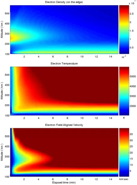
Fig. 5. Time evolution of electron parameters just on the edge of the arc, where the parallel current densities reach their peak values.
increase in the electron density in theF-region. Therefore, the Pedersen conductivity gradient increases further. The system becomes “unstable” in that sense, since the enhanced gradients introduce stronger parallel currents, more electron heating and so on and so forth. However, since our code is, in effect, nonlinear, the growth process reaches a limit after the structures have gone to a large enough amplitude.
For added context and for a better understanding of the processes involved we have introduced a description of the time evolution in Figs. 5 and 6 for two specific locations. In Fig. 5 we present the evolution of the electron density, tem-perature, and field-aligned velocity, on the edge of the arc, where the parallel currents are most intense. The changes keep pace with the increase in the conductivity gradient on the edge of the arc. Since the chemical time constants are of the order of 1 min, it is little surprise that the parallel cur-rents and the disturbances they introduce saturate after a few minutes. We can also clearly see from the figure that, on the edge of the arc, where the current densities reach their largest values, the minimum in the electron field-aligned velocity is located near theF-region peak that was present prior to the introduction of the arc.
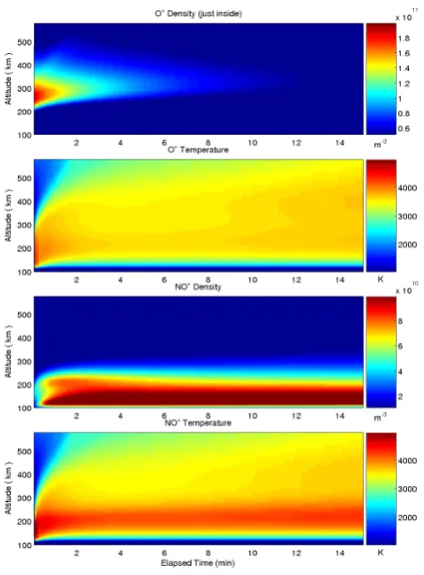
[image:8.595.48.280.67.380.2]Below 300 km, as the O+ ions are being converted into NO+ions, a secondary peak occurs in the NO+density near 200 km altitude (see Fig. 6). However, after the conversion of
Fig. 6. Time evolution of ion parameters just inside the precipitation zone, whereE-region conductivities reach their largest values.
O+ions into NO+ions, the initial peak disappears because of recombination. The electron velocity minimum follows suit and goes away with the disappearance of the density peak.
−7 −6 −5 −4 −3 100
150 200 250 300 350 400
Altitude ( km )
Electron Density
m−3
0.5 1 1.5 2 2.5 3 x 10¹¹
−7 −6 −5 −4 −3 100
150 200 250 300 350 400
Altitude ( km )
O+ Density
m−35
6 7 8 9 10 x 1010
−7 −6 −5 −4 −3 100
150 200 250 300 350 400
Altitude ( km )
Electron Temperature
K1000 2000 3000 4000 5000 6000
−7 −6 −5 −4 −3 100
150 200 250 300 350 400
Horizontal Position (km)
Altitude ( km )
NO+ Density
m−3
0.5 1 1.5 2 2.5 3 x 10¹¹
−7 −6 −5 −4 −3 100
150 200 250 300 350 400
Altitude ( km )
O+ Temperature
K1000 2000 3000 4000 5000 6000
−7 −6 −5 −4 −3 100
150 200 250 300 350 400
Horizontal Position ( km ) NO+ Temperature
K1000 2000 3000 4000 5000 6000
Fig. 7. Same as in Fig. 3, but with the addition ofE-region wave heating of electrons, following the prescription proposed by Robin-son (1986).
collision frequency between O+and neutral atomic oxygen
is relatively large and introduces a measurable difference be-tween the neutral mass-weighted averages of the atomic and molecular ions.
3.2 Case 2 – with electron wave heating using Robinson’s expression
We now present in Figs. 7 and 8 the results of our calcu-lations in the presence of wave heating rates. For our first case, we have introduced Robinson’s expressions, Eq. (9), in TRANSCAR. The new figures obtained from these calcula-tions are identical in format to Figs. 3 and 4, and the cases are identical, except for the introduction of the wave heating rate.
3.2.1 Density differences
When comparing the new results with the old, to start with we observe significant differences in the electron densities. Specifically, theE-region electron density near 120 km alti-tude nearly doubles in the precipitation region when wave heating is added (Fig. 7, top left panel) instead of being highly enhanced only near the edge of the arc in the previ-ous case (Fig. 3, top left panel). The reason for the change
Fig. 8. Same as in Fig. 4, but with the addition ofE-region wave heating of electrons, following the prescription proposed by Robin-son (1986).
is fairly simple: with a production from precipitation, a de-crease in the dissociative recombination of the molecular ions has to lead to larger densities. By contrast, outside the arc, while the recombination rate also slows down, there is no source term and the effect on the densities is considerably reduced, in spite of the elevated electron temperatures.
We also observe an increase in the electron density at about 300 km altitude in response to the O+density enhance-ment in the region of reduced electric fields. We note that the F-region enhancement is not as dramatic in the wave heated case as it was in the case without the wave heating source and that the wave heated case also extends a bit more hori-zontally. This is consistent with the O+ temperature being lower over a wider horizontal distance for the second case compared to the first.
The electron density features are otherwise common to both runs. For instance, we have a density enhancement in both cases, extending upward from the 120 km altitude re-gion on the edge of the arc.
3.2.2 Temperature differences
the wave heated case, the electrons have temperatures well in excess of 1000 K everywhere in a 10 to 20 km thick region below 120 km altitude. This, of course, is directly related to the wave heating term itself. A closer look also reveals that the 110-km altitude electron temperature is significantly structured horizontally. For instance, just outside the arc, just below∼120 km altitude, the electron temperature has a value of∼3000 K while just inside the arc the temperature has dropped to a value of∼2000 K. The change in tempera-ture occurs over a distance of about 400 m. Given the strong dependence of the wave heating rate on the electric field, this change can easily be seen to be a direct consequence of the horizontal structuring in the perpendicular electric field. The latter is present in both runs but is allowed to affect the E-region electron temperatures only in the wave heated case.
What may be more striking is a large electron temperature increase on the edge of the arc everywhere above 150 km. This increase is, in turn, directly related, through frictional heating, to an increase in the magnitude of the field-aligned current densities. The current density now reaches a magni-tude of∼550µA/m2(Fig. 8, middle right panel). This rep-resents an increase of the order of 20–30% compared to the case when electron wave heating was not considered (Fig. 4, middle right panel).
In the middle and bottom right panels of Fig. 7, we ob-serve that the O+and NO+ temperatures are also more el-evated than they were in Fig. 3. The temperatures are hor-izontally structured, as before, but they are enhanced over the case devoid of wave heating everywhere throughout the altitude range 120 km to 300 km in the horizontal interval be-ing shown. The enhancements are particularly noticeable on the outside edge of the arc, at about 130 km, where the tem-perature reaches∼5500 K for O+ and∼6000 K for NO+. By contrast, just inside the arc the temperatures decrease to
∼3800 K for O+ and∼4500 K for NO+, over a horizontal distance of approximately 400 m, respectively. The tempera-ture enhancements are due to changes introduced in the per-turbed electric field in the wave heated case. Basically, the regions of positive electric field enhancements are more pro-nounced than in the wave-heating-free case, whereas the re-gions of negative enhancements are less depressed than be-fore.
3.2.3 Electrodynamical changes
The electric field differences that we have just mentioned are, of course, associated with visible changes in the potential, as can be seen from a comparison of the middle left panels of Fig. 4 and Fig. 8. Most noticeable is a motion upward of the potential maximum in the wave heated case. The maxi-mum is now near 110 km, namely around the point where the electron temperature is also peaking. This affects the verti-cal distribution in the parallel field, in particular. The effect is most visible where it concerns the parallel currents, with the 20–30% increase in current density that we already men-tioned for the wave heated case.
The changes in the electric field are connected, in turn, to changes in the conductivity gradient, as can be readily seen from Eq. (6). Figure 8 clearly shows that the Pedersen con-ductivity in the wave heating case is nearly 5 times higher inside the arc than outside. The enhancement in the Ped-ersen conductivity inside the arc results in larger horizontal gradients on the edge of the arc. The large gradients in the conductivity is at the origin of the parallel currents’ inten-sification. We also notice that, contrary to the case without wave heating, the Pedersen conductivity is also fairly con-stant throughout the arc. The increase in the conductivity is, in large part, directly related to the large increase in the E-region electron density. There is, nevertheless, also a more minor contribution from the elevated electron temperature, as can be seen from Eqs. (14) to (16).
The enhancements in the E-region conductivities inside the arc have consequently to move more charges to the edge of the arc. A priori, this can have two different kinds of con-sequences concerning the electrodynamics. First, one could argue that with higher Pedersen conductivities, the ambient (perpendicular) electric field inside the arc should be shorted out more than in the poorer conductivity case. Alternatively, the effect could be reduced if, instead, the difference trans-lated into more intense parallel fields and parallel currents on the edge of the arc. Clearly, at least for the case that we have considered here, the second process dominates: The perpendicular electric field panels only show a small reduc-tion in the sense that the perpendicular field becomes reduced further inside the arc than in Case 1. However, the mag-nitudes of the perpendicular fields are comparable in both runs. Where parallel currents and parallel electric fields on the edge of the arc are concerned, however, we have a dif-ferent story. The parallel current densities are measurably larger in the wave heating case. This is, of course, due to the presence of stronger parallel electric fields which may be less easy to see, but are, nevertheless, very much there.
We conclude that there can be little doubt thatE-region plasma wave heating does affect the response of the plasma to sharp changes in precipitating fluxes in the presence of strong ambient electric fields. While quite visible effects are seen in various locations in the densities and temperatures, the electrodynamics at the edge of the arcs is most strongly affected. Our study of the results furthermore leads us to conclude that the enhanced parallel currents and fields are mostly the consequence of an enhancement in the horizontal (perpendicular) Pedersen conductivity gradient at the edge of the arc.
Fig. 9. Time evolution of electron parameters just on the edge of the arc, where the parallel current densities reach their peak values.
quickly. We can also see that the changes in the NO+
den-sity inside the arc are evident right from the beginning, since E-region electron heating responds immediately to applied perpendicular fields and therefore immediately slows down the NO+recombination process, thereby allowing more ions to be present.
3.3 Case 3 – with electron wave heating using the Dimant and Milikh’s expression
As stated in the Introduction, the expressions for the wave heating rate that were obtained by Robinson (1986) are dif-ferent from those obtained by Dimant and Milikh (2003). Since both formulations appear to do a reasonable job where observations are concerned, we have decided to repeat our wave heating run with the Dimant and Milikh rates, to see if whatever differences there are can have an impact on the response of the system.
It turns out that the results from the two heated runs, while not identical, are rather similar. The largest differ-ences are in the electrodynamical part, but even there, they are small. For instance, the field-aligned current density was
∼550µA/m2 when we used Robinson’s expressions, while for the Milikh and Dimant (2003) case the magnitude reaches
∼570µA/m2. This is still only a∼4% increase. The small
Fig. 10. Time evolution of ion parameters just inside the precipita-tion zone, whereE-region conductivities reach their largest values.
differences can themselves be tracked down to small changes in the conductivity distribution.
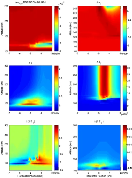
In order to more clearly assess the differences between our two wave heating cases, we have plotted in Fig. 11 the differ-ences in the electrodynamical parameters between the two runs. The Pedersen and parallel conductivities differences are shown in the top panels. The middle panels contain the electric potential (left side) and the absolute value of the dif-ferences in the field-aligned current density (right side). The bottom panel contain the differences in the perturbed perpen-dicular and parallel electric fields. The Milikh and Dimant (2003) rates produce somewhat larger temperatures than the Robinson model. This, in turn, give somewhat larger Peder-sen conductivities in the former case, which results in some-what larger parallel electric fields and somesome-what less contrast in the perpendicular electric fields on each side of the edge of the arc. These trends are similar to the differences that were observed between the heated and non-heated case, but are, of course, of much smaller amplitudes.
[image:11.595.48.280.67.380.2]Fig. 11. Differences between various electrodynamical parameters for the two different wave heating rate expressions (case 2 results minus case 3 results) that we have considered in this work. Same presentation format as in Fig. 4 but with the differences instead of the actual quantities.
other two runs into which the wave heating were parameter-ized somewhat differently. The results are shown in Figs. 12 and 13. They illustrate more precisely the small differences between the two heating runs (some curves are exactly on top of each other) while showing the effect ofE-region wave heating on the results in these two key locations.
4 Summary and conclusion
We have used our two-dimensional model of small-scale electrodynamics near auroral arcs to assess the impact of electron heating by plasma waves in the auroralE-region. Just as we did in the No¨el et al. (2000) study, we focused on arcs with sharp cutoffs in precipitation with little structure inside the precipitation, region, since these are the kinds of arcs that are associated with strong parallel current densities on their edges and are very sensitive to Pedersen conductivity gradients.
In the present work, electron temperatures that are boosted byE-region wave heating will, in turn, boost the electron density inside the precipitating regions by decreasing the re-combination rate of the molecular ions. This increases the
1011
50 100 150 200 250 300 350 400
m−3
altitude (km)
Electron density after 5 minutes no Rob. D&M
1010
1011
150 200 250 300 350 400
O+ density after 5 minutes
altitude (km)
m−3
1011
50 100 150 200 250 300 350 400
NO+ density after 5 minutes
altitude (km)
m−3
0 2000 4000 6000 8000 50
100 150 200 250 300 350 400
Te after 5 minutes
altitude (km)
Kelvin
0 2000 4000 6000 8000 50
100 150 200 250 300 350 400
TO+ after 5 minutes
altitude (km)
Kelvin
0 2000 4000 6000 8000 50
100 150 200 250 300 350 400
TNO+ after 5 minutes
altitude (km)
[image:12.595.310.547.66.387.2]Kelvin
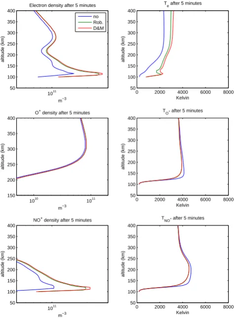
Fig. 12. Density and temperature profiles 5 min after the introduc-tion of an electric field and of precipitaintroduc-tion, taken just on the edge of the arc, in the region of large parallel current densities.
contrast between the Pedersen conductivity inside the arc versus outside the arc. In turn, this drives a horizontal di-vergence in perpendicular currents near the edge of the arcs, which ends up triggering stronger parallel current densities in that region. Additional feedback effects are introduced because the parallel currents create, in turn, a heating of elec-trons through friction, thereby affecting collision frequencies and densities, which in turn again affects the conductivity of the medium. With our imposed 200-m cutoff scale for pre-cipitation, the resulting effects are very large, increasing al-ready substantial parallel current densities of several hundred µA m−2by up to 30%.
1011
50 100 150 200 250 300 350 400
m−3
altitude (km)
Electron density after 5 minutes no Rob. D&M
1010
1011
150 200 250 300 350 400
O+ density after 5 minutes
altitude (km)
m−3
1011
50 100 150 200 250 300 350 400
NO+ density after 5 minutes
altitude (km)
m−3
0 2000 4000 6000 8000 50
100 150 200 250 300 350 400
Te after 5 minutes
altitude (km)
Kelvin
0 2000 4000 6000 8000 50
100 150 200 250 300 350 400
TO+ after 5 minutes
altitude (km)
Kelvin
0 2000 4000 6000 8000 50
100 150 200 250 300 350 400
TNO+ after 5 minutes
altitude (km)
[image:13.595.48.287.66.392.2]Kelvin
Fig. 13. Density and temperature profiles 5 min after the introduc-tion of an electric field and of precipitaintroduc-tion, taken just inside the arc, in the region of peakE-region electron densities.
amplitude, small-scale plasma structures can play an impor-tant role not so much by directly affecting the electric field that creates them, but more by modifying the fields through changes in the conductivities, with conductivity gradients in-troduced indirectly through chemical effects.
Acknowledgements. This research was funded by research grants
to JMN and JPSTM from the National Science and Research Engi-neering Council of Canada.
Topical Editor M. Lester thanks Y. Dimant and another referee for their help in evaluating this paper.
References
Albritton, D. L., Dotan, I., Lindinger, W., McFarland, M., Tellinghuisen, J., and Fehsenfeld, F. C.: Effects of ion speed dis-tributions in flow-drift tube studies on ion-neutral reactions, J. Chem. Phys., 66, 410–421, 1977.
Blelly, P.-L. and Schunk, R. W.: A comparative study of the time-dependent standard 8-, 13- and 16-moment transport formula-tions of the polar wind, Ann. Geophys., 11, 443–469, 1993. Blelly, P.-L., Robineau, A., Lilensten, J., and Lummerzheim, D.:
8-moment fluid models of the terrestrial high latitude iono-sphere between 100 and 3000 km, Solar terrestrial energy pro-gram (STEP): handbook of ionospheric models, 53–72, 1996.
Blelly, P.-L., Lilensten, J., Robineau, A., Fontanari, J., and Alcayd´e, D.: Calibration of a numerical ionospheric model with EISCAT observations, Ann. Geophys., 14, 1375–1390, 1996,
SRef-ID: 1432-0576/ag/1996-14-1375.
Blelly, P.-L., Lathuill`ere, C., Emery, B., Lilensten, J., Fontanari, J., and Alcayd´e, D.: An extended TRANSCAR model including ionospheric convection: simulation of EISCAT observations us-ing inputs from AMIE, Ann. Geophys., 23, 419–431, 2005, SRef-ID: 1432-0576/ag/2005-23-419.
Dimant, Y. S. and Milikh, G. M.: Model of anomalous electron heating in theEregion, I: basic theory, J. Geophys. Res., 108, 1350, doi:10.1029/2002JA009,524, 2003.
Lilensten, J., Kofman, W., Wisenberg, J., Oran, E., and Devore, C.: Ionization efficiency due to primary and secondary photoelec-trons: a numerical model, Ann. Geophys., 7, 83–90, 1989. Lilensten, J. and Blelly, P. L.: The TEC and F2 parameters as tracers
of the ionosphere and thermosphere, J. of Atmos. Terr. Phys., 64, 775–793, 2002.
Loranc, M. and St.-Maurice, J.-P.: A time-dependent gyro-kinetic model of thermal ion upflows in the high-latitudeF-region, J. Geophys. Res., 99, 17 429–17 451, 1994.
Lummerzheim, D. and Lilensten, J.: Electron transport and energy degradation in the ionosphere: evaluation of the numerical solu-tion, comparison with laboratory experiments and auroral obser-vations, Ann. Geophys., 12, 1039–1051, 1994,
SRef-ID: 1432-0576/ag/1994-12-1039.
Milikh, G. M. and Dimant, Y. S.: Kinetic model of electron heating by turbulent electric field in theEregion, Geophys. Res. Lett., 29, doi:10.1029/2001GL013,935, 2002.
Milikh, G. M. and Dimant, Y. S.: Model of anomalous electron heating in theEregion, II: detailed numerical modeling., J. Geo-phys. Res., 108, 1351, doi:10.1029/2002JA009,527, 2003. No¨el, J.-M., St.-Maurice, J.-P., and Blelly, P.-L.: Nonlinear model
of short-scale electrodynamics in the auroral ionosphere, Ann. Geophys., 18, 1128–1144, 2000,
SRef-ID: 1432-0576/ag/2000-18-1128.
Otto, A. and Zhu, H.: Fluid plasma simulation of coupled sys-tems: Ionosphere and magnetosphere, in: Space Plasma Simu-lation, Proc. International School for Space SimuSimu-lation, (Eds.) Buechner, J., Dunn, G. T., and Scholer, M., 6th International School/Symposium on Space Plasma Simulation, Copernicus Gessellschaft, Germany, 96, 2001.
Rees, M. H.: Physics and chemistry of the upper atmosphere, Cam-bridge atmospheric and space science series, CamCam-bridge Univer-sity Press, Cambridge, United Kingdom, 1989.
Robinson, T. R.: Towards a self-consistent nonlinear theory of radar auroral backscatter, J. Atmos. Terr. Phys., 48, 417–423, 1986. Schlegel, K. and St.-Maurice, J.-P.: Anomalous heating of the polar
E-region by unstable plasma waves, 1. Observation, J. Geophys. Res., 86, 1447–1452, 1981.
Schunk, R. W. and Nagy, A. F.: Ionospheres. Physics, plasma physics, and chemistry, Cambridge atmophseric and space sci-ence series, Cambridge University Press, Cambridge, United Kingdom, 2000.
Sheehan, C. and St.-Maurice, J.-P.: The dissociative recombi-nation of N+2, O+2, and NO+: Rate coefficients for ground state and vibrationally excited ions, J. Geophys. Res., A03302 doi:10.1029/2003JA010132, 2004.
St.-Maurice, J.-P.: A unified theory of anomalous resistivity and Joule heating effects in the presence ofE-region irregularities, J. Geophys. Res., 92, 4533–4542, 1987.
-region, in: Polar cap Dynamics and High Latitudes turbulence: SPI Conference proceedings and Reprint series, No. 8, 1988, Sci-entific Publishers, Cambridge, Mass., 323–348, 1990a.
St.-Maurice, J.-P.: Electron heating by plasma waves in the high latitudeE-region: Theory, in: Advances in Space Research, vol. 10, Pergamon Press 239–249, 1990b.
St.-Maurice, J.-P. and Hamza, A. M.: A new nonlinear approach to the theory ofEregion irregularities, J. Geophys. Res., 106, 1751–1759, 2001.
St.-Maurice, J.-P. and Hanson, W. B.: Ion frictional heating at high latitudes and its possible use for an in situ detemination of neu-tral thermospheric winds and temperatures, J. Geophys. Res., 87, 7580–7602, 1982.
St.-Maurice, J.-P. and Laher, R.: Are observed broadband plasma wave amplitudes large enough to explain the enhanced electron temperatures of the high-latitudeE region?, J. Geophys. Res., 90, 2843–2850, 1985.
St.-Maurice, J.-P. and Laneville, P. J.: The reaction rate of O+with O2, N2, and NO under highly disturbed auroral conditions., J. Geophys. Res., 103, 17 519–17 521, 1998.
St.-Maurice, J.-P. and Torr, D. G.: The effect of relative speed dis-tributions on the reaction rates of O+with N2, O2and NO in the thermosphere, J. Geophys. Res., 83, 969–977, 1978.
St.-Maurice, J.-P., Kofman, W., and James, D.: In-situ generation of intense parallel fields in the lower ionosphere, J. Geophys. Res., 101, 335–356, 1996.
Wickwar, V. B., Lathuill`ere, C., Kofman, W., and Lejeune, G.: Ele-vated electron temperatures in the auroralElayer measured with the chatanika radar, J. Geophys. Res., 86, 4721–4730, 1981. Zhu, H., Otto, A., Lummerzheim, D., Rees, M. H., and Lanchester,