On the linear fuzzy model associated with Caputo–Fabrizio operator

(1)

R E S E A R C H

Open Access

On the linear fuzzy model associated with

Caputo–Fabrizio operator

R. Abdollahi

1

_{, A. Khastan}

2,3*

_{, J.J. Nieto}

2

_{and R. Rodríguez-López}

2

*_{Correspondence:}

[email protected]

2_{Instituto de Matemáticas,}

Departamento de Estatística, Análisis Matemático y Optimización, Facultade de Matemáticas, Universidade de Santiago de Compostela, Santiago de Compostela, Spain

3_{Department of Mathematics,}

Institute for Advanced Studies in Basic Sciences (IASBS), Zanjan, Iran Full list of author information is available at the end of the article

Abstract

In this paper, we introduce the fuzzy Caputo–Fabrizio operator under generalized Hukuhara diﬀerentiability concept. In this setting, we study the linear fuzzy fractional initial value problems and present the general form of their solutions. Some examples are given to illustrate our results.

Keywords: Caputo–Fabrizio operator; Fuzzy fractional initial value problem; Generalized diﬀerentiability; Fuzzy diﬀerential equations

1 Introduction

During the last decades, the subject of fractional calculus has gained an increase of impor-tance, mainly because it has become a powerful tool with accurate and successful results in modeling several complex phenomena in numerous seemingly diverse and widespread fields of science and engineering [14, 17, 18]. Fractional calculus is not only a productive and emerging field, it also represents a new philosophy to constructing and applying a cer-tain type of nonlocal operators to real world problems. The ones possessing both nonlo-cal effects as well as uncertainty behaviors represent interesting phenomena. Researchers started to combine, in an intelligent way, the notions “fractional” and “fuzzy”, therefore a hybrid operator, called fuzzy fractional operator, emerged [1].

In one of the earliest works, Agarwal et al. [2] took the initiative and introduced fuzzy fractional calculus to handle fractional-order systems with uncertain initial values or un-certain relationships between parameters. Arshad and Lupulescu [4, 5] have deduced some existence and uniqueness results for fuzzy fractional differential equations under Riemann–Liouville derivative. In [13], the authors used Schauder fixed point theorem to study the existence of solution for fuzzy fractional differential equations.

It has been demonstrated that the fractional-order modeling is particularly useful to rep-resent systems where the memory plays a significant role, this quality is the most signif-icant advantage. The Riemann–Liouville definition entails physically unacceptable initial conditions; conversely, for the Caputo representation, the initial conditions are expressed in terms of integer-order derivatives having direct physical significance [1]. These defi-nitions have the disadvantage that their kernels have singularity, therefore both defini-tions cannot accurately describe the full effect of the memory. Due to this inconvenience, Caputo and Fabrizio in [10] presented a new definition of fractional derivative without singular kernel, the Caputo–Fabrizio (CF) fractional derivative. This fractional operator

(2)

possesses very interesting properties; for instance, this definition allows for the descrip-tion of mechanical properties related with damage, fatigue, material heterogeneities, and structures at different scales [1]. Later Losada and Nieto [16] introduced the fractional integral corresponding to this new concept. They also modified the definition of Caputo and Fabrizio and proposed a new definition for fractional operator that we use in this pa-per. Properties and applications of this new fractional operator are reviewed in detail in [1, 6]. A model of resistance, inductance, capacitance circuit using the Caputo–Fabrizio operator with fractional order is proposed in [6]. In [11], the authors applied the Caputo– Fabrizio operator to the diffusion and the diffusion–advection equation. In [7], Baleanu et al. studied the existence of solutions for some infinite coefficient-symmetric Caputo– Fabrizio fractional integro-differential equations. A new scheme to find the fuzzy approx-imate solution of fractional differential equations under uncertainty with Caputo-type derivative based on the generalized Hukuhara differentiability is presented in [3]. Recently, in [20], Salahshour et al. generalized the concept of fractional derivative in the sense of Caputo–Fabrizio derivative for interval-valued function under uncertainty. They studied three real-world systems, such as the falling body problem, Basset and Decay problem, using fractional interval differential equations under Caputo–Fabrizio derivative.

In [12], the authors studied first-order linear fuzzy differential equations and presented the general form of solutions. In this paper, we introduce fuzzy Caputo–Fabrizio fractional operator under the generalized Hukuhara differentiability concept. We investigate a linear fuzzy fractional initial value problem with new Caputo–Fabrizio operator and present the form of the solution in the general case.

The paper is organized as follows. In Sect. 2, we recall some basic knowledge of fuzzy cal-culus and fractional calcal-culus. In Sect. 3, we recall some results for linear fractional diﬀer-ential equations with Caputo–Fabrizio operator. In Sect. 4, we study a linear fuzzy model, and in Sect. 5 some examples are given.

2 Preliminaries

In this section, we give some deﬁnitions and useful results and introduce the necessary notation which will be used throughout the paper. Most of it can be found, for example, in [8].

LetXbe a nonempty set. A fuzzy setuinXis characterized by its membership function

u:X→[0, 1], whereu(x) is interpreted as the degree of membership of an elementxin the fuzzy setufor eachx∈X.

Deﬁnition 2.1 A fuzzy number is a function such asu:R−→[0, 1] satisfying the follow-ing properties:

(i) uis normal, that is, there existsx0∈Rsuch thatu(x0) = 1;

(ii) uis a fuzzy convex set, i.e.,u((1 –λ)x+λy)≥min{u(x),u(y)},∀x,y∈R,λ∈[0, 1]; (iii) uis upper semi-continuous;

(iv) [u]0₌_cl{x_∈_R;_u₍_x_{) > 0}_}_{is compact.}

The set of all fuzzy real numbers is denoted byRF. Given a fuzzy numberu∈RF and

0 <r≤1, we obtain ther-level set ofuby [u]r₌_{s_∈_R_|_u₍_s₎_≥_r}_{and the support of}_u

as [u]0₌_cl{s_∈_R_|_u₍_s_{) > 0}_}_{. For any}_r_∈_{[0, 1], due to the properties imposed on the set of} fuzzy numbers, we have that [u]r_{is a bounded closed interval. The notation [}_u_]r_{= [}_ur_,_ur_]

(3)

For givenu,v∈RF andλ∈R, we deﬁne the sumu+vand the productλuby the

stan-dard level-set operations [u+v]r_{= [}_u_]r_{+ [}_v_]r_{, [}_λu_]r₌_λ_[_u_]r_,_∀r_∈_{[0, 1], where [}_u_]r_{+ [}_v_]r

means the usual addition of two intervals (subsets) ofRandλ[u]r_{means the usual}

prod-uct between a scalar and a subset ofR. The metric structure is given by the Hausdorﬀ distanceD:RF×RF→R+∪ {0},

D[u,v] = sup

r∈[0,1]

maxur–vr,ur–vr, u,v∈RF.

Remark2.2 The following properties are well known [8]:

1. (RF,D)is a complete metric space. 2. D[u+w,v+w] =D[u,v],∀u,v,w∈RF. 3. D[ku,kv] =|k|D[u,v],∀k∈R.

4. D[u+v,w+e]≤D[u,w] +D[v,e],∀u,v,w,e∈RF.

Foru,v∈RF, if there existsw∈RF such thatu=v+w, thenwis called the H-diﬀerence

ofu,vand it is denoted byuv. We use this notationuvto represent the H-diﬀerence ofuandv, which is diﬀerent, in general, fromu–v=u+ (–1)v.

Deﬁnition 2.3([9]) LetF: (a,b)−→RF. Fixt0∈(a,b). We say thatFis generalized dif-ferentiable att0if there exists an elementF(t0)∈RF such that either

(i) for allh> 0suﬃciently close to 0, the H-diﬀerencesF(t0+h)F(t0),

F(t0)F(t0–h)exist and the limits (in the metricD)

lim

h→0+

F(t0+h)F(t0)

h =hlim→0+

F(t0)F(t0–h)

h =F(t0)

or

(ii) for allh> 0suﬃciently close to 0, the H-diﬀerencesF(t0)F(t0+h),

F(t0–h)F(t0)exist and the limits (in the metricD)

lim

h→0+

F(t0)F(t0+h) –h =hlim→0+

F(t0–h)F(t0)

–h =F(t0).

In the previous definition, case (i) corresponds to the H-derivative introduced in [19], so this differentiability concept is a generalization of the Hukuhara derivative. In [9], the authors consider four cases for derivatives. Here we only consider the two first cases of Definition 5 in [9]. In the other cases, the derivative is trivial because it is reduced to a crisp element.

Deﬁnition 2.4 LetF: (a,b)−→RF. We say that F is (i)-diﬀerentiable on (a,b) if F is

differentiable in the sense (i) of Definition 2.3 on (a,b). Similarly, we say thatF is (ii )-differentiable on (a,b) ifFis differentiable in the sense (ii) of Definition 2.3 on (a,b).

Theorem 2.5([8]) Let F: (a,b)−→RFand put[F(t)]r= [F(t;r),F(t;r)]for each r∈[0, 1]. (i) IfFis(i)-diﬀerentiable,thenFandFare diﬀerentiable functions and

[F(t)]r_{= [}_F₍_t_;_r_),_F₍_t_;_r_)]_.

(ii) IfFis(ii)-diﬀerentiable,thenFandFare diﬀerentiable functions and

(4)

LetT⊂Rbe an interval. We denote byC(T,RF) the space of all continuous fuzzy

func-tions onT. Also, we denote byL1₍_T_,_R

F) the space of all fuzzy functionsf :T−→RFwhich

are Lebesgue integrable on the bounded intervalTofR.

Deﬁnition 2.6([4]) IfF: [a,b]−→RFis Riemann integrable on [a,b], then the

paramet-ric representation of its integral is given by

b

a

F(t;r)dt=

b

a

F(t;r)dt,

b

a

F(t;r)dt

, r∈[0, 1].

Deﬁnition 2.7([15]) Givenb> 0,f∈H1_(0,_b_{), and 0 <}_α_{< 1, the Caputo fractional} deriva-tive off of orderαis given by

C_Dα

f(t) = 1

(1 –α)

t

0

(t–s)–αf (s)ds, t≥0.

By changing the kernel (t–s)–α_{by the function}_exp_(– α

1–α(t–s)) and

1

(1–α)by 1

√

2π(1–α2₎,

one obtains the new Caputo–Fabrizio operator of order 0 <α< 1, which has been recently introduced by Caputo and Fabrizio in [10] as

CF_Dα

f(t) =(2 –α)M(α) 2(1 –α)

t

0

exp

– α

1 –α(t–s)

f (s)ds, t≥0,

whereM(α) is a normalization constant depending onα.

According to the new deﬁnition, it is clear that iff is a constant function, thenDα_f_{= 0 as}

in the usual Caputo derivative. The main difference between the old and the new definition is that, contrary to the old definition, the new kernel has no singularity fort=s.

In [16], the authors have introduced the new associated fractional integral and then they obtained thatM(α) =_2–2_α, so they proposed a new deﬁnition as follows.

Deﬁnition 2.8 [16] Let 0 <α< 1. The fractional Caputo–Fabrizio operator of orderαof a functionf is given by

Dαf(t) = 1 (1 –α)

t

0

exp

– α

1 –α(t–s)

f (s)ds, t≥0.

In the following, we introduce the deﬁnition of Caputo–Fabrizio operator for fuzzy number valued functions.

Deﬁnition 2.9 Letf : [0,a]−→RF be generalized diﬀerentiable withf ∈C((0,a],RF)∩ L1_((0,_a_),_R

F). The generalized fuzzy Caputo–Fabrizio operator of the fuzzy-valued

func-tionf is deﬁned as

Dα_f ₍_t_{) =} 1

(1 –α)

t

0

exp

– α

1 –α(t–s)

f (s)ds, t≥0, (1)

(5)

Deﬁnition 2.10 Letf : [0,a]−→RFbe generalized diﬀerentiable withf ∈C((0,a],RF)∩ L1_((0,_a_),_R

F). We say thatfis (i,α)-diﬀerentiable if (Dαf)(t;r) = [(Dαf)(t;r), (Dαf)(t;r)] and

is (ii,α)-diﬀerentiable if (Dα_f₎₍_t_;_r_{) = [(}_Dα_f₎₍_t_;_r_{), (}_Dα_f₎₍_t_;_r_)].

Theorem 2.11 Let f : [0,a]−→RF be generalized diﬀerentiable at t0with f ∈C((0,a], RF)∩L1((0,a),RF).Then:

(i) f is(i)-differentiable att0ifff is(i,α)-differentiable att0.

(ii) f is(ii)-differentiable att0ifff is(ii,α)-differentiable att0.

Proof Using Theorem 2.5 and Deﬁnitions 2.6, 2.9, and 2.10, the proof is

straightfor-ward.

3 Linear fractional differential equation

Losada and Nieto in [16] studied the initial value problem

⎧ ⎨ ⎩

Dα_f₍_t_{) =}_σ₍_t_), _t_≥_0,

f(0) =f0∈R,

(2)

using the Caputo–Fabrizio operator. The authors in [16] applied the Laplace transform to both sides of (2) to obtain the solution. In this paper, we suppose that the appropriate conditions for applying the Laplace transform hold. For example, in (2), this is possible if

f ∈H1_(0,_∞_),_f_∈_C_([0,_∞_)),_σ_∈_C_([0,_∞_{)) and}CF_Dα_f_,_σ_{are functions of exponential order.}

We recall the following result from [16].

Theorem 3.1 Let0 <α< 1.Then the unique solution of the initial value problem(2)is given by

f(t) =f0+ (1 –α)

σ(t) –σ(0) +αI1σ(t), t≥0,

where I1_σ₍_t_{) =}t 0σ(s)ds.

Now, we consider the following linear fractional diﬀerential equation:

Dα_∗f(t) =λf(t) +u(t), f(0) =f0,t≥0, (3)

whereλ,f0∈Randuis diﬀerentiable for allt≥0. From Theorem 3.1, we have [16]

f(t) =f0+ (1 –α)

λf(t) –f(0) +u(t) –u(0)+α

t

0

[λf +u](s)ds, t≥0. (4)

So

(1 –p)f(t) –qI1f(t) = (1 –p)f0+ (1 –α)

u(t) –u(0) +αI1u(t), t≥0, (5)

(6)

Ifp= 1, then we have

–qI1f(t) = (1 –α)u(t) –u(0) +αI1u(t), t≥0,

so

f(t) =1 –α –q u(t) –

α

qu(t), t> 0. (6)

Ifp= 1, then we have

f(t) – q 1 –pI

1_f₍_t_{) =}_σ_˜₍_t_), _t_≥_0, ₍₇₎

where

˜

σ(t) =f0+ 1 –α

1 –p

u(t) –u(0) + α 1 –pI

1_u₍_t_), _t_≥_0.

The caseλ= 0 is trivial, since in this casep=q= 0 and, from (7), we obtain

f(t) =σ˜(t), (8)

which coincides with the expression in Theorem 3.1 takingσ=u. Ifλ= 0, we have

f(t) –λI˜ 1f(t) =σ˜(t), t≥0,

whereλ˜=_1–q_p, hence

f (t) =λf˜ (t) +σ˜ (t), t≥0.

Thus, we have obtained an ordinary diﬀerential equation, which has a unique solution if we consider an initial condition [16].

4 Linear fuzzy model with Caputo–Fabrizio operator

In this section, we consider the fuzzy initial value problem

⎧ ⎨ ⎩

Dα_f₍_t_{) =}_λf₍_t_{) +}_u₍_t_),

f(0) =f0, (9)

wheref,u:I→RFare continuous fuzzy functions,uis generalized diﬀerentiable onI,f0∈ RFandλ∈R, and in such a way that functionsf,f,u,u,Dαf,Dαf have Laplace transform.

(7)

a system of classical initial value problems. Then using Theorem 2.11 and (4), we obtain the (i,α)-diﬀerentiable and (ii,α)-diﬀerentiable solutions to (9).

We study the existence of (i,α)- and (ii,α)-solutions to problem (9) by distinguishing three casesλ> 0,λ< 0, andλ= 0.

CaseI. Letλ> 0. Suppose thatf(t) is (i,α)-diﬀerentiable. Then (9) is equivalent to

Dα_f₍_t_),_Dα_f₍_t₎ ₌_λf₍_t_{) +}_u₍_t_),_λf₍_t_{) +}_u₍_t₎_.

So, we have

⎧ ⎨ ⎩

Dα_f₍_t_{) =}_λf₍_t_{) +}_u₍_t_), _f_{(0) =}_f

0,

Dα_f₍_t_{) =}_λf₍_t_{) +}_u₍_t_), _f_{(0) =}_f_0.

Then, by equation (5), we have

⎧ ⎨ ⎩

(1 –p)f(t) –qI1_f₍_t_{) = (1 –}_p₎_f

0+ (1 –α)(u(t) –u(0)) +αI1u(t), (1 –p)f(t) –qI1_f₍_t_{) = (1 –}_p₎_f

0+ (1 –α)(u(t) –u(0)) +αI1u(t),

(10)

wherep=λ(1 –α) andq=λα.

Ifp= 1, then, by diﬀerentiating both sides of (10), we have

f(t) =1 –α –q u(t) –

α qu(t),

and similarly

f(t) =1 –α –q u(t) –

α qu(t).

Then we obtain

f(t),f(t)=1 –α –q

u(t),u(t)α

q

u(t),u(t),

provided the level sets define a valid fuzzy function. So, ifu(t) is (i)-differentiable, then we do not find any fuzzy solutionf(t), unlessu(t) is a crisp function onI. In case thatu(t) is (ii)-differentiable, then [u(t)] = [u(t),u(t)] and we have the solution as follows:

f(t) =1 –α –q u(t)

α

qu(t), f(0) =f0,

provided that the H-diﬀerence exists.

Remark4.1 It is easy to see that ifdiam(u(t))≥ α

1–αdiam(u(t)), thenf(t)≤f(t),∀t≥0.

Indeed, in this case,diam(u(t)) =u(t) –u(t), so that we havef(t) –f(t) =1–α

q diam(u(t)) –

α

(8)

Ifp< 1, then using (7), we obtain

f(t) – q 1 –pI

1_f₍_t_{) =}_f_{(0) +}1 –α 1 –p

u(t) –u(0) + α 1 –pI

1_u₍_t_). ₍₁₁₎

If we putλ˜=_1–q_p, then

f(t) –λI˜ 1f(t) =f(0) +(1 –α)λ˜

q

u(t) –u(0) +λα˜

q I

1_u₍_t_). ₍₁₂₎

By diﬀerentiating both sides of (12), we obtain

f (t) –λf˜ (t) =(1 –α)λ˜

q u(t) + ˜ λα

q u(t). (13)

So, consideringf(0) =f0, we have

f(t) =eλ˜t

t

0

e–λ˜s

(1 –α)λ˜

q u(s) + ˜ λα

q u(s)

ds+f0

=eλ˜t

(1 –α)λ˜

q

t

0

e–λ˜su(s)ds+λα˜

q

t

0

e–λ˜su(s)ds+f0

=(1 –α)λ˜

q

u(t) –eλ˜tu(0) +eλ˜t(1 –α)λ˜

2₊_α_λ˜

q

t

0

e–λ˜su(s)ds+f0eλ˜t.

Therefore,

f(t) =(1 –α)λ˜

q

u(t) –eλ˜t_u₍₀₎ ₊_eλ˜tλ˜2α q2

t

0

e–˜λs_u₍_s₎_ds₊_f

0eλ˜t,

and similarly

f(t) =(1 –α)λ˜

q

u(t) –eλ˜tu(0) +eλ˜tλ˜

2_α

q2

t

0

e–˜λsu(s)ds+f0eλ˜t.

Sincep< 1 andλ˜> 0, then the solution is

f(t) =(1 –α)λ˜

q

u(t)eλ˜tu(0) +eλ˜tλ˜

2_α

q2

t

0

e–λ˜su(s)ds+f0eλ˜t,

provided that the H-diﬀerence exists.

On the other hand, if we considerp> 1, sinceλ˜< 0, similarly to the casep< 1, we obtain

f(t) = –(1 –α)λ˜

q

eλ˜tu(0)u(t) +eλ˜tλ˜

2_α

q2

t

0

e–λ˜su(s)ds+f0eλ˜t,

provided that the H-diﬀerence exists. Thus, we have proved the following result.

(9)

(i) Ifp= 1andu(t)is(ii)-diﬀerentiable,thenf(t) =1–_–_qαu(t)α_qu(t),f(0) =f0.

(ii) Ifp< 1,thenf(t) =(1–_qα)λ˜(u(t)eλ˜t_u_{(0)) +}_eλ˜tλ˜2α

q2

t

0e–

˜

λs_u₍_s₎_ds₊_f

0eλ˜t,provided that

the H-diﬀerence exists.

(iii) Ifp> 1,thenf(t) = –(1–_qα)˜λ(eλ˜t_u₍₀₎_u₍_t_{)) +}_eλ˜tλ˜2α

q2

t

0e

–λ˜s_u₍_s₎_ds₊_f

0e˜λt,provided

that H-diﬀerences exist.

Now, suppose thatf(t) is (ii,α)-diﬀerentiable. Then (9) is equivalent to

Dαf(t),Dαf(t) =λf(t) +u(t),λf(t) +u(t). (14)

So, we have ⎧ ⎨ ⎩

Dα_f₍_t_{) =}_λf₍_t_{) +}_u₍_t_), _f_{(0) =}_f_0,

Dα_f₍_t_{) =}_λf₍_t_{) +}_u₍_t_), _f_{(0) =}_f_0.

From Theorem 3.1, we have ⎧

⎨ ⎩

f(t) =f(0) + (1 –α)(λf(t) +u(t) –λf(0) –u(0)) +αI1₍_λf ₊_u₎₍_t_),

f(t) =f(0) + (1 –α)(λf(t) +u(t) –λf(0) –u(0)) +αI1₍_λf ₊_u₎₍_t_).

By hypothesis, sinceuis generalized differentiable onI, thenu(t) andu(t) are differ-entiable onI. So differentiating both sides of the last equations, we obtain the systems of ordinary differential equations

⎧ ⎨ ⎩

f (t) –pf (t) = (1 –α)u(t) +qf(t) +αu(t),

f (t) –pf (t) = (1 –α)u(t) +qf(t) +αu(t).

Then, by solving this system forp= 1, it is easy to see that ⎧

⎨ ⎩

f (t) =_1–pq_p2f(t) +

q

1–p2f(t) +

αp2

q(1–p2₎u(t) +

αp

1–p2u(t) +

αp

q(1–p2₎u(t) +_1–α_p2u(t),

f (t) =_1–pq_p2f(t) +

q

1–p2f(t) +

αp2

q(1–p2₎u(t) +

αp

1–p2u(t) +

αp

q(1–p2₎u(t) +_1–α_p2u(t).

So,

f (t)

=m

p 1

1 p

f(t)

+mα

q

_p2

qu(t) +pu(t) + p

qu(t) +u(t) p2

qu(t) +pu(t) + p

qu(t) +u(t)

,

wherem=_1–q_p2.

By the variation of constants formula for ordinary diﬀerential equations, we have

f(t)

=epmt

cosh(mt) sinh(mt)

sinh(mt) cosh(mt) × f(0) f(0) + t 0

e–pms

cosh(ms) –sinh(ms) –sinh(ms) cosh(ms)

b(s)

ds

(10)

where

b(t) =mα

q

p2

qu(t) +pu(t) + p

qu(t) +u(t)

(15)

and

b(t) =mα

q

p2

qu(t) +pu(t) + p

qu(t) +u(t)

. (16)

Then we have

f(t)

=epmt

cosh(mt) sinh(mt)

sinh(mt) cosh(mt)

×

f(0) +₀te–pms_[_b₍_s₎_cosh₍_ms_{) –}_b₍_s₎_sinh₍_ms_)]_ds f(0) +₀te–pms_[–_b₍_s₎_sinh₍_ms_{) +}_b₍_s₎_cosh₍_ms_)]_ds

.

So that

f(t) =epmtcosh(mt)

f(0) +

t

0

e–pmsb(s)cosh(ms) –b(s)sinh(ms)ds

+epmtsinh(mt)

f(0) +

t

0

and

f(0) +

t

0

+epmtsinh(mt)

f(0) +

t

0

.

Remark 4.3 It is easy to check that for p < 1, when u(t) is (ii)-diﬀerentiable and

diam(u(t))≥ α

1–αdiam(u(t)), then

b(t) =mαp

q

p

qu(t) +u(t)

–mα

q

p

qu(t) +u(t)

(17)

is such that level-wise H-diﬀerence exists. Since, in this casediam(u(t)) =u(t) –u(t), and by (15)–(16), we have

b(t) –b(t) = –αp 2_m

q2 diam

u(t) +αpm

q diam

u(t)

+αpm

q2 diam

u(t) –αm

q diam

u(t)

=1 –α 1 +pdiam

u(t) – α 1 +pdiam

u(t) ≥0.

(11)

Therefore, ifp< 1 (or equivalentlym> 0), the (ii,α) solution to (9) is given by

f(0) +

t

0

–epmtsinh(mt)

f(0) +

t

0

,

provided that the level-wise H-differences define a fuzzy interval fort> 0, whereb(t) is defined in (17).

Remark 4.4 Since for m > 0, cosh(mt) ≥ sinh(mt), then for every C ∈ RF, the

H-diﬀerenceepmtcosh(mt)Cepmtsinh(mt)Cexists. Also the H-diﬀerenceepmtcosh(mt)C

–epmt_sinh₍_mt₎_C_{exists level-wise.}

Ifp> 1 (or equivalentlym< 0), similarly to the previous case, the (ii,α)-solution is given by

f(0) +

t

0

e–pmsb(s)cosh(ms)b(s)sinh(ms)ds

+epmtsinh(mt)

f(0) +

t

0

.

So, we have proved the following result.

Theorem 4.5 Letλ> 0,m= _1–q_p2,b(t)be a valid fuzzy function deﬁned as in(17)and

u(t)be(ii)-diﬀerentiable with the propertydiam(u(t))≥_1–α_αdiam(u(t))for t> 0.Then the following assertions are valid:

(i) Ifp< 1,then the(ii,α)-solution to(9)is given by

f(0) +

t

0

–epmtsinh(mt)

f(0) +

t

0

,

t≥0,

provided that the level-wise diﬀerences deﬁne a fuzzy interval fort> 0. (ii) Ifp> 1,then the(ii,α)-solution to(9)is given by

f(0) +

t

0

+epmtsinh(mt)

f(0) +

t

0

,

t≥0,

(12)

CaseII. Letλ< 0. Suppose thatf(t) is (i,α)-diﬀerentiable. Then (9) is equivalent to the following system of ordinary diﬀerential equations:

⎧ ⎨ ⎩

Dα_f₍_t_{) =}_λf₍_t_{) +}_u₍_t_), _f_{(0) =}_f_0,

Dα_f₍_t_{) =}_λf₍_t_{) +}_u₍_t_), _f_{(0) =}_f

0.

Similarly to the second part of Case I, we have

f(0) +

t

0

e–pmsb˜(s)cosh(ms) –b˜(s)sinh(ms)ds

+epmtsinh(mt)

f(0) +

t

0

(18)

and

f(t) =epmtsinh(mt)

f(0) +

t

0

+epmtcosh(mt)

f(0) +

t

0

, (19)

wherem= q 1–p2 and

˜

b(t) =mα

q

p2

qu(t) +pu(t) + p

qu(t) +u(t)

(20)

and

˜

b(t) =mα

q

p2

qu(t) +pu(t) + p

qu(t) +u(t)

. (21)

First, we consider p< –1. It is easy to check that, whenu(t) is (ii)-diﬀerentiable and

diam(u(t))≥_1–α_αdiam(u(t)), then

˜ b(t) =

αp2_m

q2 u(t)–

αpm q u(t)

+

αpm

q2 u(t)–

αm q u(t)

(22)

is such that the corresponding level-wise H-diﬀerences exist. This fact is due to the fol-lowing. In this case,diam(u(t)) =u(t) –u(t) and, using (20)–(21), we have

˜

b(t) –b˜(t) = αp 2_m

q2 diam

u(t) –αpm

q diam

u(t)

– αpm

q2 diam

u(t) +αm

q diam

u(t)

= α– 1 1 +pdiam

u(t) + α 1 +pdiam

u(t)

(13)

Therefore, since we suppose 1 +p< 0, so ifdiam(u(t))≥_1–α_αdiam(u(t)), then the level sets ofb˜(t) are valid intervals. It is easy to check that, whenu(t) is (i)-diﬀerentiable,b˜(t) is not a fuzzy function, unlessu(t) is crisp for everyt.

Thus, ifp< –1, thenm> 0 and, by equations (18)–(19), we have the (i,α)-solution as follows:

f(0) +

t

0

–epmt_sinh₍_mt₎

f(0) +

t

0

e–pms_b˜₍_s₎_cosh₍_ms_{) –}_b˜₍_s₎_sinh₍_ms₎_ds

,

provided level-wise differences define a fuzzy interval fort> 0, whereb˜(t) is defined as in (22).

Now, suppose that –1 < p< 0 (or equivalently m < 0). In this case, if u(t) is (i )-diﬀerentiable, then, using (20)–(21), we can writeb˜(t) as a fuzzy function

˜

b(t) =αm

q u(t) + αpm

q2 u(t) +

αp2_m

q2 u(t). (23)

On the other hand, ifu(t) is (2)-diﬀerentiable, then by (20)–(21)

˜ b(t) =

αpm

q u(t)– αp2m

q2 u(t)

+

αm

q u(t)– αpm

q2 u(t)

, (24)

where the level-wise H-diﬀerences exist when_1–α_αdiam(u(t))≥diam(u(t)). Then, for –1 <p< 0, we obtain

f(0) +

t

0

e–pmsb˜(s)cosh(ms) ˜b(s)sinh(ms)ds

+epmtsinh(mt)

f(0) +

t

0

,

where b˜(t) is defined by (23) or (24) (according to the type of differentiability ofu(t)), provided that the level-wise H-differences define proper fuzzy functions. In consequence, we have proved the following result.

Theorem 4.6 Suppose thatλ< 0.

(i) Letp< –1,u(t)be(ii)-diﬀerentiable and satisfyingdiam(u(t))≥_1–α_αdiam(u(t)). Then the(i,α)-solution to problem(9)is given by

f(0) +

t

0

–epmtsinh(mt)

f(0) +

t

0

,

provided the H-diﬀerence exists,whereb˜(t)is given in(22).

(ii) Let–1 <p< 0.Ifuis(i)-diﬀerentiable andb˜(t)is deﬁned in(23),or ifuis

(14)

is a valid fuzzy function in(24),then the(i,α)-solution to problem(9)is given by

f(0) +

t

0

+epmtsinh(mt)

f(0) +

t

0

,

provided the H-diﬀerence exists.

Suppose thatλ< 0 andf(t) is (ii,α)-diﬀerentiable. Then (9) is equivalent to ⎧

⎨ ⎩

Dα_f₍_t_{) =}_λf₍_t_{) +}_u₍_t_), _f_{(0) =}_f_0,

Dα_f₍_t_{) =}_λf₍_t_{) +}_u₍_t_), _f_{(0) =}_f_0.

Then, using (5), we have

(1 –p)f(t) –qI1f(t) = (1 –p)f0+ (1 –α)

u(t) –u(0) +αI1u(t), (25)

and similarly forf(t). Sinceλ< 0 and 0 <α< 1, then 1 –p> 1, so that, using (7), we get

f(t) – q 1 –pI

1_f₍_t_{) =}_f_{(0) +}1 –α 1 –p

u(t) –u(0) + α 1 –pI

1_u₍_t_).

Similarly to the previous case, proceeding analogously to (11), we obtain

f(t) =(1 –α)λ˜

q

2_α

q2

t

0

e–˜λsu(s)ds+f0eλ˜t,

and similarly

f(t) =(1 –α)λ˜

q

2_α

q2

t

0

e–˜λsu(s)ds+f0eλ˜t,

whereλ˜=_1–q_p. Hence we deduce

f(t) =

f0eλ˜t–

(1 –α)λ˜ λα e

˜

λt_u₍₀₎

–

(1 –α)λ˜ λα u(t) +e

˜

λt λ˜2 λ2_α

t

0

e–λ˜s_u₍_s₎_ds

,

provided that the H-diﬀerences exist. So, we have the following result.

Theorem 4.7 Forλ< 0,the(ii,α)-solution to problem(9)is given by

f(t) =

f0eλ˜t–

(1 –α)λ˜ λα e

˜

λt_u₍₀₎

–

(1 –α)λ˜ λα u(t) +e

˜

λt λ˜2 λ2_α

t

0

e–λ˜su(s)ds

,

(15)

CaseIII. Letλ= 0. Letf(t) be (i,α)-diﬀerentiable. Then problem (9) is equivalent to

Dαf(t),Dαf(t) =u(t),u(t) , f(0),f(0) = (f0,f0).

So, we have ⎧ ⎨ ⎩

Dα_f₍_t_{) =}_u₍_t_), _f_{(0) =}_f_0,

Dα_f₍_t_{) =}_u₍_t_), _f_{(0) =}_f

0.

So, by Theorem 3.1, we obtain ⎧

⎨ ⎩

f(t) =f(0) + (1 –α)(u(t) –u(0)) +α₀tu(s)ds,

f(t) =f(0) + (1 –α)(u(t) –u(0)) +α₀tu(s)ds.

So, the (i,α)-solution to (9) is given by

f(t) =f(0) + (1 –α)u(t)u(0) +α

t

0

u(s)ds,

provided that the H-diﬀerences exist. To obtain (ii,α)-solution, we have ⎧

⎨ ⎩

f(t) =f(0) + (1 –α)(u(t) –u(0)) +α₀tu(s)ds,

f(t) =f(0) + (1 –α)(u(t) –u(0)) +α₀tu(s)ds.

So the (ii,α)-solution to (9) is given by

f(t) =f(0)–

(1 –α)u(t)u(0) +α

t

0

u(s)ds

,

provided that the H-diﬀerences exist. So, we have the following result.

Theorem 4.8 The(i,α)- and(ii,α)-diﬀerentiable solutions to the problem

⎧ ⎨ ⎩

Dα_f₍_t_{) =}_u₍_t_), _t_≥_0,

f(0) =f0∈RF

are given by

f(t) =f(0) + (1 –α)u(t)u(0) +α

t

0

u(s)ds

and

f(t) =f(0)–

(1 –α)u(t)u(0) +α

t

0

u(s)ds

,

(16)

5 Examples

In this section, we provide several examples to illustrate the main results.

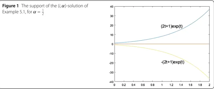
Example5.1 Letλ= 1 andu(t) = (–et, 0,et) be a triangular fuzzy number valued function. Thenλ˜= 1 and we haveur₍_t_{) = (}_r_{– 1)}_et_and_ur₍_t_{) = (1 –}_r₎_et_{. So, (9) is written as follows:}

⎧ ⎨ ⎩

CF_Dα

∗f(t) =f(t) + (–et, 0,et), f(0) = (–1, 0, 1)∈RF.

(26)

We see thatp= 1 –α< 1, so by Theorem 4.2-(ii), the (i,α)-solution to (26) is

f(t) = 1

αtu(t) +f(0)e t₌

t α+ 1

–et, 0,et .

In this case H-diﬀerence u(t)et_u_{(0) exists trivially. For} _α₌ 1

2, the support of (i,α )-solution is shown in Fig. 1. Sinceu(t) is not (ii)-diﬀerentiable, we cannot use Theorem 4.5 to obtain (ii,α)-solution.

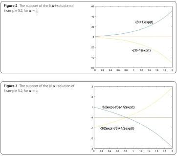
Example5.2 Letλ= –1 andu(t) = (–et_{, 0,}_et_{) be a triangular fuzzy number valued}

func-tion. Thenλ˜=_2––α_α< 0, –1 <p< 0,m=_2––1_α< 0,ur₍_t_{) = (}_r_{– 1)}_et_{, and}_ur₍_t_{) = (1 –}_r₎_et_.

So, equation (9) is equivalent to

⎧ ⎨ ⎩

CF_Dα

∗f(t) = –f(t) + (–et, 0,et), f(0) = (–1, 0, 1)∈RF.

(27)

So, using Theorem 4.6, the (i,α)-solution is

f(t) =

1 + t

α

–et, 0,et ,

which, forα=1₃, is shown in Fig. 2.

(17)

Figure 2The support of the (i,α)-solution of Example 5.2, forα=1₃

Figure 3The support of the (ii,α)-solution of Example 5.2, forα=1₂

For (ii,α)-solution withα=1

2 andt∈[0, 3

4ln3], by Theorem 4.7, we have

f(t) =

3 2e

–t

3 _–1

2e

t

(–1, 0, 1),

whose support is shown in Fig. 3.

Acknowledgements

This work has been partially supported by Agencia Estatal de Investigación (AEI) of Spain under grant MTM201675140-P, and XUNTA de Galicia under grants GRC2015-004 and R2016-022, and and co-ﬁnanced by the European Community fund FEDER.

Funding Not applicable. List of Abbreviations Not applicable.

Availability of data and materials

Data sharing not applicable to this article as no datasets were generated or analysed during the current study. Competing interests

The authors declare that they have no competing interests. Authors’ contributions

All authors contributed equally and signiﬁcantly in writing this article. All authors read and approved the ﬁnal manuscript. Author details

1_{Department of Mathematics, University of Mohaghegh Ardabili, Ardabil, Iran.}2_{Instituto de Matemáticas, Departamento}

de Estatística, Análisis Matemático y Optimización, Facultade de Matemáticas, Universidade de Santiago de Compostela, Santiago de Compostela, Spain.3_{Department of Mathematics, Institute for Advanced Studies in Basic Sciences (IASBS),}

(18)

Publisher’s Note

Springer Nature remains neutral with regard to jurisdictional claims in published maps and institutional aﬃliations.

Received: 16 February 2018 Accepted: 28 May 2018

References

1. Agarwal, R.P., Baleanu, D., Nieto, J.J., Torres, D.F., Zhou, Y.: A survey on fuzzy fractional diﬀerential and optimal control nonlocal evolution equations. J. Comput. Appl. Math. (2017). https://doi.org/10.1016/j.cam.2017.09.039

2. Agarwal, R.P., Lakshmikantham, V., Nieto, J.J.: On the concept of solution for fractional diﬀerential equations with uncertainty. Nonlinear Anal.72, 2859–2862 (2010)

3. Ahmadian, A., Salahshour, S., Ali-Akbari, M., Ismaila, F., Baleanu, D.: A novel approach to approximate fractional derivative with uncertain conditions. Chaos Solitons Fractals104, 68–76 (2017)

4. Arshad, S.: On existence and uniqueness of solution of fuzzy fractional diﬀerential equations. Iran. J. Fuzzy Syst.10, 137–151 (2013)

5. Arshad, S., Lupulescu, V.: On the fractional diﬀerential equations with uncertainty. Nonlinear Anal.74, 3685–3693 (2011)

6. Atangana, A., Alkahtani, B.S.: Extension of the resistance, inductance, capacitance electrical circuit to fractional derivative without singular kernel. Adv. Mech. Eng.7, 1–6 (2015)

7. Baleanu, D., Mousalou, A., Rezapour, S.: On the existence of solutions for some infinite coefficient-symmetric Caputo-Fabrizio fractional integro-differential equations. Bound. Value Probl.2017, 145 (2017)

8. Bede, B.: Mathematics of Fuzzy Sets and Fuzzy Logic. Springer, London (2013)

9. Bede, B., Gal, S.G.: Generalizations of the diﬀerentiability of fuzzy-number-valued functions with applications to fuzzy diﬀerential equations. Fuzzy Sets Syst.151, 581–599 (2005)

10. Caputo, M., Fabrizio, M.: A new deﬁnition of fractional derivative without singular kernel. Prog. Fract. Diﬀer. Appl.1(2), 1–13 (2015)

11. Gómez-Aguilar, J.F., López-López, M.G., Alvarado-Martínez, V.M., Reyes-Reyes, J., Adam-Medina, M.: Modeling diﬀusive transport with a fractional derivative without singular kernel. Physica A447, 467–481 (2016)

12. Khastan, A., Nieto, J.J., Rodríguez-López, R.: Variation of constant formula for ﬁrst order fuzzy diﬀerential equations. Fuzzy Sets Syst.177, 20–33 (2011)

13. Khastan, A., Nieto, J.J., Rodríguez-López, R.: Schauder ﬁxed-point theorem in semilinear spaces and its application to fractional diﬀerential equations with uncertainty. J. Fixed Point Theory Appl.2014, 21 (2014).

https://doi.org/10.1186/1687-1812-2014-21

14. Kilbas, A.A., Srivastava, H.M., Trujillo, J.J.: Theory and Applications of Fractional Diﬀerential Equations. Elsevier, Amsterdam (2006)

15. Lakshmikantham, V., Vatsala, A.S.: Basic theory of fractional diﬀerential equations. Nonlinear Anal.69, 2677–2682 (2008)

16. Losada, J., Nieto, J.J.: Properties of a new fractional derivative without singular kernel. Prog. Fract. Diﬀer. Appl.1(2), 87–92 (2015)

17. Oldham, K.B., Spanier, J.: The Fractional Calculus. Academic Press, New York (1974) 18. Podlubny, I.: Fractional Diﬀerential Equations. Academic Press, San Diego (1999)

19. Puri, M.L., Ralescu, D.A.: Diﬀerentials of fuzzy functions. J. Math. Anal. Appl.91, 552–558 (1983)