DEPARTMENT OF INFORMATION ENGINEERING AND COMPUTER SCIENCE
ICT International Doctoral School
LEARNING WITH SHARED INFORMATION FOR IMAGE
AND VIDEO ANALYSIS
Gaowen Liu
Advisor
Prof. Nicu Sebe
Universit`a degli Studi di Trento
Publications
This thesis consists of the following publications:
• Chapter 2:
Gaowen Liu, Yan Yan, Ramanathan Subramanian, Jingkuan Song, Guoyu
Lu, Nicu Sebe: Active Domain Adaptation with Noisy Labels for
Multi-media Analysis. World Wide Web 19(2): 199-215, 2016
• Chapter 3:
Gaowen Liu, Yan Yan, Elisa Ricci, Yi Yang, Yahong Han, Stefan Winkler,
Nicu Sebe: Inferring Painting Style with Multi-Task Dictionary Learning.
International Joint Conference on Artificial Intelligence (IJCAI):
2162-2168, 2015
Gaowen Liu, Yan Yan, Jingkuan Song, Nicu Sebe: Minimizing dataset
bias: Discriminative multi-task sparse coding through shared subspace
learning for image classification. International Conference on Image
Pro-cessing (ICIP): 2869-2873, 2014
• Chapter 4:
Yan Yan, Elisa Ricci, Gaowen Liu, Nicu Sebe: Egocentric Daily Activity
Recognition via Multitask Clustering. IEEE Transactions on Image
Pro-cessing 24(10): 2984-2995, 2015
The following are the papers published during the course of the Ph.D but not
included in this thesis:
• Gaowen Liu, Yan Yan, Chenqiang Gao, Wei Tong, Alexander G.
Haupt-mann, Nicu Sebe:The Mystery of Faces: Investigating Face Contribution
for Multimedia Event Detection. ACM International Conference on
• Yan Yan, Elisa Ricci, Ramanathan Subramanian, Gaowen Liu, Oswald
Lanz, Nicu Sebe: A Multi-Task Learning Framework for Head Pose
Esti-mation under Target Motion. IEEE Transactions on Pattern Analysis and
Machine Intelligence 38(6): 1070-1083, 2016
• Yan Yan, Yi Yang, Deyu Meng, Gaowen Liu, Wei Tong, Alexander G.
Hauptmann, Nicu Sebe: Event Oriented Dictionary Learning for Complex
Event Detection. IEEE Transactions on Image Processing 24(6):
1867-1878, 2015
• Yan Yan, Yi Yang, Haoquan Shen, Deyu Meng, Gaowen Liu, Alexander
G. Hauptmann, Nicu Sebe: Complex Event Detection via Event Oriented
Dictionary Learning. AAAI Conference on Artificial Intelligence (AAAI):
3841-3847, 2015
• Yan Yan, Haoquan Shen,Gaowen Liu, Zhigang Ma, Chenqiang Gao, Nicu
Sebe: GLocal tells you more: Coupling GLocal structural for feature
se-lection with sparsity for image and video classification. Computer Vision
and Image Understanding, vol 124: 99-109, 2014
• Yan Yan, Elisa Ricci, Ramanathan Subramanian,Gaowen Liu, Nicu Sebe:
Multitask Linear Discriminant Analysis for View Invariant Action
Recog-nition. IEEE Transactions on Image Processing 23(12): 5599-5611, 2014
• Yan Yan, Elisa Ricci,Gaowen Liu, Ramanathan Subramanian, Nicu Sebe:
Clustered Multi-task Linear Discriminant Analysis for View Invariant
Color-Depth Action Recognition. International Conference on Pattern
Recogni-tion (ICPR): 3493-3498, 2014
• Chenqiang Gao, Deyu Meng, Wei Tong, Yi Yang, Yang Cai, Haoquan
Shen, Gaowen Liu, Shicheng Xu, Alexander G. Hauptmann:Interactive
Represen-tation. ACM International Conference on Multimedia Retrieval (ICMR),
2014
• Yan Yan, Gaowen Liu, Elisa Ricci, Nicu Sebe: Multi-task linear
discrim-inant analysis for multi-view action recognition. International Conference
on Image Processing (ICIP): 2842-2846, 2013
• Yan Yan, Zhongwen Xu, Gaowen Liu, Zhigang Ma, Nicu Sebe: GLocal
structural feature selection with sparsity for multimedia data
Contents
1 Introduction 1
1.1 Contribution of the Thesis . . . 3
1.2 Overview of the Thesis . . . 3
2 Active Domain Adaption 5 2.1 Introduction . . . 6
2.2 Related Work . . . 8
2.2.1 Active Learning . . . 8
2.2.2 Domain Adaptation . . . 9
2.2.3 Learning with Noisy Labels . . . 11
2.3 Active Domain Adaptation with Noisy Labels . . . 12
2.3.1 SVM-based Domain Adaptation . . . 12
2.3.2 Multiclass Active Learning . . . 14
2.3.3 Modeling with Noisy Labels . . . 15
2.3.4 Framework . . . 16
2.4 Experiments . . . 18
2.4.1 Cross-domain Headpose Dataset . . . 18
2.4.2 Cross-domain Berkeley Web Image Dataset . . . 23
2.5 Conclusion . . . 25
3.1.1 Introduction . . . 30
3.1.2 Related Work . . . 33
3.1.2.1 Automatic Analysis of Paintings . . . 33
3.1.2.2 Dictionary and Multi-task Learning . . . 33
3.1.3 Learning Style-specific Dictionaries . . . 34
3.1.3.1 Feature Extraction from Paintings . . . 34
3.1.3.2 Multi-task Dictionary Learning . . . 36
3.1.3.3 Optimization . . . 38
3.1.4 Experimental Results . . . 40
3.1.4.1 Dataset . . . 40
3.1.5 Experimental Setup and Baselines . . . 41
3.1.5.1 Quantitative Evaluation . . . 42
3.2 Discriminative multi-task dictionary learning for image classi-fication . . . 46
3.2.1 Introduction . . . 47
3.2.2 Problem Formulation . . . 49
3.2.2.1 Multi-task Sparse Coding . . . 49
3.2.2.2 Discriminative Multi-task Sparse Coding for Classification . . . 50
3.2.3 Experiments . . . 52
3.2.3.1 Datasets . . . 52
3.2.3.2 Experiment Settings . . . 52
3.2.3.3 Quantitative Evaluation . . . 53
3.2.4 Conclusion . . . 56
4 Activity recognition via Multi-task Clustering 57 4.1 Introduction . . . 58
4.2 Related Work . . . 61
4.2.2 Supervised Multi-task Learning . . . 62
4.2.3 Multi-task Clustering . . . 63
4.3 Multi-task Clustering for First-person Vision Activity Recognition 64 4.3.1 Motivation and Overview . . . 64
4.3.2 Earth Mover’s Distance Multi-task Clustering . . . 66
4.3.2.1 Optimization . . . 68
4.3.3 Convex Multi-task Clustering . . . 70
4.3.3.1 Optimization . . . 70
4.3.4 Features Extraction in Egocentric Videos . . . 73
4.3.4.1 FPV office dataset . . . 74
4.3.4.2 FPV home dataset . . . 75
4.4 Experimental Results . . . 76
4.4.1 Synthetic data experiments . . . 76
4.4.2 FPV Results . . . 78
4.4.2.1 FPV office dataset . . . 79
4.4.2.2 FPV home dataset . . . 81
4.4.3 Discussion . . . 83
4.5 Conclusions . . . 84
5 Conclusion and Future Work 87 5.1 Conclusion . . . 87
5.2 Future Work . . . 88
List of Tables
2.1 Source domain - webcamimages. . . 26
2.2 Source domain - dslr images. . . 26
2.3 Source domain - amazonimages. . . 26
3.1 Structure of the DART dataset. . . 41
3.2 Comparison with baseline methods. . . 43
3.3 Evaluation on different features combinations. . . 43
3.4 Recognition accuracy (5 training samples per class) . . . 55
4.1 Parameters used in the synthetic data experiments. . . 77
List of Figures
1.1 The overview of this thesis. . . 2
2.1 Framework for Active Domain Adaptation with Noisy Labels:
labelled source, labelled and unlabelled target data are used to
train the transfer classifier. Active learning is performed to
se-lect unlabelled target data to be labelled by the expert. . . 16
2.2 4-view exemplar from the (a) CLEAR and (b) DPOSE datasets.
Automatically extracted face crops are shown on the bottom
right inset. . . 19
2.3 Classification accuracies with (left) single view and (right) 4
views. . . 20
2.4 Confusion matrix over 24 classes for active DA after 30 rounds. 21
2.5 Evaluating active DA classification error with different loss
func-tions. . . 22
2.6 Evaluating our active DA framework with batch mode querying
by varying number of queried samples/class/round. . . 22
2.7 Evaluating active domain adaptation with noisy labels modeling
strategy. . . 23
2.8 Exemplars from the Berkeley web image dataset. (from top
to bottom) Web (amazon), digital SLR camera (high resolution
3.1 Given the images belonging to the Baroque, Renaissance,
Im-pressionism,Cubism,Postimpressionism,Modernart movements,
can you detect which ones correspond to the same style1? . . . . 31
3.2 Extracted features: color (light blue), composition (red) and
lines (blue). . . 35
3.3 Examples of paintings from the DART dataset. Each image is
associated with a detailed description containing year, artist and
painting name. . . 40
3.4 (Left) Confusion Matrix on DART dataset. (Middle)
Perfor-mance at varying dictionary size land subspace dimensionality
s. (Right) Visualization of contributions of each component for
the Cubism style. Different colors represent different
compo-nents,i.e. color (green), composition (red) and lines (blue). . . 44
3.5 Visualization of learned dictionaries when using raw pixels
fea-tures for (left)Cubismand (right) Renaissance. . . 45
3.6 The phylogenetic tree reflecting the similarities among artists.
(Figure is best viewed under zoom). . . 46
3.7 Framework of Discriminative Multi-task Sparse Coding through
Shared Subspace Learning. . . 48
3.8 Example images from AwA dataset (top) and Caltech-101 dataset
(bottom). . . 53
3.9 Performance comparisions (5 training samples per class used)
(a) Different dictionary size on Caltech-101 dataset; (b) Diff
er-ent dictionary size on AwA dataset; (c) Different subspace size
on Caltech-101 and AwA dataset. . . 54
3.10 Sensitivity study of parameters λ1 and λ2 (5 training samples
4.1 Overview of our multi-task clustering approach for FPV activity
recognition (Figure best viewed in color). . . 58
4.2 Feature extraction pipeline on the FPV office dataset. Some
frames corresponding to the actions read, browse and copy are
shown together with the corresponding optical flow features
(top) and eye-gaze patterns depicted on the 2-D plane (bottom).
It is interesting to observe the different gaze patterns among
these activities. . . 71
4.3 Samples generated in the synthetic data experiments (different
colors represent different clusters). . . 78
4.4 Clustering results on synthetic data for different methods.
Meth-ods based on linear kernel are separated from those with
Gaus-sian kernel. (Figure is best viewed in color). . . 79
4.5 FPV Office dataset. Temporal video segmentation on the
sec-ond sequence of subject-3 (13 minutes): comparison of different
methods. (Best viewed in color). . . 80
4.6 FPV Office dataset. Confusion matrices using saccade+motion
features obtained with (left) KEMD-MTC and (right) CMTC
methods. . . 81
4.7 Comparison of different methods using (left) bag of features
and (right) temporal pyramid features on FPV home dataset.
(Figure is best viewed in color). . . 81
4.8 Temporal video segmentation on a sequence of the FPV home
dataset. (The edge of the shaded area at the bottom of each
subfigure indicates the current frame). . . 83
4.9 FPV home dataset: performance variations of EMD-MTC and
KEMD-MTC at different values ofλusing (left) bag of features
4.10 Sensitivity study of parametersλt and λ2 in CMTC using (left)
Chapter 1
Introduction
Image and video recognition is a fundamental and challenging problem in
com-puter vision, which has progressed tremendously fast recently. In the real world,
a realistic setting for image or video recognition is that we have some classes
containing lots of training data and many classes that contain only a small
amount of training data. Therefore, how to use the frequent classes to help
learning the rare classes is an open question. Learning with shared
informa-tion is an emerging topic which can solve this problem. There are different
components that can be shared during concept modelling and machine
learn-ing procedure, such as sharlearn-ing generic object parts, sharlearn-ing attributes, sharlearn-ing
transformations, sharing regularization parameters and sharing training
exam-ples,etc. For example, representations based on attributes define a finite
vocab-ulary that is common to all categories, with each category using a subset of the
attributes. Therefore, sharing some common attributes for multiple classes will
benefit the final recognition system.
In this thesis, we investigate some challenging image and video recognition
problems under the framework of learning with shared information. My Ph.D
research comprised of two parts. The first part focuses on the two domains
(source and target) problems where the emphasis is to boost the recognition
Figure 1.1: The overview of this thesis.
domain. The second part focuses on multi-domains problems where all domains
are considered equally important. This means we want to improve performance
for all domains by exploring the useful information across domains. Fig.1.1
shows the overview of this thesis. These two parts can be summarized as
learn-ing with shared information. In particular, we investigate three topics to achieve
this goal in the thesis, which are active domain adaptation, multi-task learning,
1.1
Contribution of the Thesis
To sum up, this thesis makes the following contributions towardslearning with
shared information:
• For two domains (source and target) image recognition problem, an
ac-tive domain adaptation framework is proposed to illustrate the power of
learning with shared information.
• For multiple domains (parallel tasks), we introduce the idea of learning
style-specific dictionaries. A novel multi-task dictionary learning is
pro-posed for automatic analysis of painting image recognition.
• For multiple domains (parallel tasks), we also propose an unsupervised
approach, a multi-task clustering framework, for the first-person vision
activity video recognition.
1.2
Overview of the Thesis
In Chapter 2, we begin our research from image recognition problem using
domain adaptation which involves transferring useful information from source
domain to the target domain to boost recognition performance. Moreover, we
integrate domain adaptation (DA) with active leaning (AL) which helps to
min-imize the effort for the acquisition of labelled data. We perform extensive
ex-periments on different datasets to evaluate our strategy.
Multi-task learning is another approach for learning with shared information.
Multi-task learning is an approach to inductive transfer that improves
general-ization by using the domain information contained in the training signals of
related tasks as an inductive bias. It does this by learning tasks in parallel while
using a shared representation. What is learned for each task can help other tasks
approach by uncovering a shared subspace of different datasets. We also investi-gate a multi-task dictionary learning approach for inferring painting styles. The
results show that multi-task dictionary learning achieve better performance for
image recognition.
To step further, we move on our research on discovering and extracting
rele-vant patterns from videos. In Chapter 4, we consider the videos collected from
wearable cameras of several people performing daily activities. We notice that,
videos continuously record several hours of human life. The data is
hetero-geneous and labelling them is an intensive and boring task requiring extensive
human labour. In order to tackle the problem, an unsupervised multi-task
clus-tering framework is proposed for video activity analysis in Chapter 4.
In summary, Chapters 2, 3, 4 present three different strategies to perform
learning with shared information. Chapter 5 presents the conclusions and the
Chapter 2
Active Domain Adaption
1Supervised learning methods require sufficient labelled examples to learn a
good model for classification or regression. However, available labelled data
are insufficient in many applications. Active learning (AL) and domain
adapta-tion (DA) are two strategies to minimize the required amount of labelled data
for model training. AL requires the domain expert to label a small number of
highly informative examples to facilitate classification, while DA involves
tun-ing the source domain knowledge for classification on the target domain. In this
chapter, we demonstrate how AL can efficiently minimize the required amount
of labelled data for DA. Since the source and target domains usually have
dif-ferent distributions, it is possible that the domain expert may not have sufficient
knowledge to answer each query correctly. We exploit our active DA framework
to handle incorrect labels provided by domain experts. Experiments with
mul-timedia data demonstrate the efficiency of our proposed framework for active
DA with noisy labels.
2.1
Introduction
In machine learning, supervised methods require sufficient labelled examples
in order to learn a good model. However, it is difficult to acquire sufficient
labelled data in many real world applications. Moreover, labelling is an
inten-sive task requiring exteninten-sive human labor. In order to tackle this problem,
sev-eral approaches have been proposed. Semi-supervised learning aims to exploit
the consistency between labelled and unlabelled data for classification. Active
learning (AL) focuses on selecting a small set of essential examples for
query-ing labels from domain experts. Domain adaptation (DA, also called Transfer
learning) facilitates classification when the training (source) and test (target)
data are from different domains. Domain adaptation uses the knowledge
ac-quired from a large number of labelled source examples and a few labelled
target examples for classification in the target domain.
DA algorithms (see [76] for a survey) seek to combine limited target data
with the source data in order to adapt to the target domain. However, they
typically tend to choose target examples randomly without considering which
samples are most informative for classification in the target domain. Therefore,
one question that needs to be examined is whether and how we can efficiently
label target data for DA? Considering that the goal of both domain adaptation
and active learning is to minimize labor-intensive data labelling, it would be
worthwhile to integrate DA and AL in a single framework.
To our knowledge, very few works studied how to minimize the amount of
labelled target data, especially under noisy labelling. A theoretical study on the
number of labelled examples required to learn all targets to achieve an
arbitrar-ily specified accuracy is presented in [118]. Two active transfer learning
algo-rithms that allow for changes in all marginal and conditional distributions with
the additional assumption that these changes are smooth are proposed in [100].
DA scenarios. [88] propose active transfer learning, but their approach is
lim-ited by the unlikely assumption that identical prediction labels are generated for
a target example by the out-of-domain (source) and in-domain (target)
classi-fiers. Additionally, the error rate of the transfer classifier is not bounded, and
only binary classification is considered here. Extending active transfer
learn-ing to multi-class classification as in this work, the upper-bound error rate
in-creases considerably and consequently, the domain-adaptive classifier cannot
classify correctly anymore. In this chapter, we investigate an adaptive DA
al-gorithm within an AL framework able to cope with label noise. We also extend
the binary classification to a multi-class classification problem through
error-correcting output coding. We investigate how AL helps to minimize the
num-bers of labelled data for DA even under noisy labelling. Experiments on
real-world datasets for head-pose estimation and image classification demonstrate
the efficacy of our proposed framework. To sum up, this chapter makes the
following contributions:
• An active domain adaptation framework under noisy labelling is proposed,
and is shown to be effective for multimedia analysis;
• We integrate active learning with domain adaptation for a multi-class
set-ting through error correcset-ting output coding;
• The proposed framework is general, and potentially applicable to many
multimedia problems.
The chapter is organized as follows. Section 2.2 reviews related work from
the perspective of active learning, domain adaptation and learning with noisy
la-bels. Section 2.3 details active domain adaptation with noisy lala-bels. Section 2.4
presents experimental results on head pose estimation and image classification,
2.2
Related Work
In this section, we review related work in the areas of active learning, domain
adaptation and learning with noisy labels.
2.2.1 Active Learning
Active learning (AL) involves asking the domain expert to label a small number
of most-informative examples to facilitate classification. Based on query
sce-narios, AL can be divided into three types of settings: (i) Membership query
synthesis, (ii) stream-based selective sampling and (iii) pool-based sampling.
The pool-based scenario has been studied for many real-world problems in
ma-chine learning and computer vision. Uncertainty sampling is a common
ap-proach in AL. Distance from hyperplane for margin-based classifiers has been
used as a measure of uncertainty in previous works. [96] provided a theoretical
motivation for SVM-based AL using the notion of a version space. [103]
pro-posed a unified multi-class AL approach through error-correcting output coding
based on the ’best worst case’, which approximates the expected loss function
with the smallest loss function among all the possible labels.
[44] extended the Fisher information framework to the batch-mode setting
for binary logistic regression. [87] studied the problem of using several
heuris-tics that take into account estimates of both oracle and model-uncertainty, and
showed that data can be improved by selective repeated labelling. However,
their analysis assumed both were equally and consistently noisy and annotation
was a noisy process over some underlying true label. [59] introduced a novel
criterion that requested a partial ordering for a set of examples that minimized
the total rank margin in attribute space, subject to a visual diversity constraint.
Existing AL strategies can have uneven performance, being efficient on some
datasets but ineffective on others, or inconsistent just between runs on the same
hierar-chical sub-query evaluation algorithm to combat this variability and to use the
potential of expected error reduction. [32] developed an efficient active
learn-ing framework based on convex programmlearn-ing, which can select multiple
sam-ples at a time for annotation. Unlike the state-of-the-art, their algorithm can be
used in conjunction with any classifier type, including sparsity-based classifiers
(SRC). [45] presented a collaborative computational model for AL with
multi-ple human oracles. This approach leads not only to an ensemble kernel machine
robust to noisy labels, but also to a principled label-quality measure detecting
irresponsible labellers online.
[58] presented a novel multi-level AL approach to reduce the human
an-notation effort for training robust scene classification models. Different from
most existing AL methods that can only query labels for selected instances
at the class level, their approach established a semantic framework that
pre-dicted scene labels based on a latent object-based image representation, and
was capable of querying labels at two different levels– the scene-class level
and the latent object-class level. [120] proposed a semi-supervised batch mode
multi-class AL algorithm for visual concept recognition. [18] proposed a novel
convex, semi-supervised multi-label feature selection algorithm applicable to
large-scale datasets.
2.2.2 Domain Adaptation
Traditional machine learning algorithms are based on the assumption that
ing and test data share the same distribution in feature space. When the
train-ing and test distributions are different, the classification accuracy drops
signif-icantly. In such cases, domain adaptation (DA) between the two domains is
desirable. DA assumes that the training and testing data could be from different
domains and distributions. It is motivated by the fact that people can
intelli-gently apply knowledge learned previously to solve new problems efficiently.
the training (or source) and test (or target) domains. [76] identified three main
research issues in DA: (i) what to transfer, (ii) how to transfer, and (iii) when
to transfer. ‘What to transfer’ examines which knowledge can be transferred
across domains or tasks. After discovering which knowledge can be transferred,
learning algorithms are developed to describe the process of ‘how to transfer’.
‘When to transfer’ studies the situations where the knowledge could be
trans-ferred, in order to guard against negative knowledge transfer that could hurt
classification performance on the target domain.
There are several DA approaches. Instance-transfer involves re-weighting
some source data for use in the target domain under the assumption that source
data can be reused in the target domain ([24, 46, 124]).
Feature-representation-transfer attempts to find a ‘good’ feature representation that reduces the diff
er-ence between the source and target domains as well as the classification/regression
error ([6, 26]). Parameter-transfer involves discovery of shared parameters or
priors between the source and target models which can benefit from transfer
learning ([10, 33, 79]). Relational-knowledge-transfer builds a mapping of
re-lational knowledge between the source and target domains ([72]).
In essence, transfer learning adapts useful source information to efficiently
classify in the target domain whose attributes vary with respect to the source.
[26] proposed a feature replication method to augment features for transfer
learning. [84] and [53] proposed a method for domain adaption using metric
learning by generating cross-domain constraints. [24] used a boosting
frame-work ([37]) to re-weight the importance of source and target samples for DA.
[124] extended the transfer boosting framework to include information from
multiple sources. [116] adapted DA by learning a delta function between the
source and target domains based on SVMs. This method seeks the target
de-cision boundary which is close to the source dede-cision boundary. [29] extended
this method via multiple kernel learning by learning kernels that minimize the
image attribute adaptation. [128] proposed a DA framework for still-to-motion
Adaptation (SMA) for human action recognition. [41] proposed finding a
low-dimensional optimal consensus representation from multiple heterogeneous
fea-tures for multi-view transfer learning. [42] proposed a sparse multi-label
learn-ing method to circumvent the visually polysemous barrier of multiple tags.
2.2.3 Learning with Noisy Labels
Nowadays, with the exponential growth of user-generated web images and videos,
there has been an increasing interest in learning models that can handle noisy
la-bels for supervised learning. This is a practical problem due to the uncontrolled
environments in which humans label data. Given the importance of learning
from noisy labels, a great deal of progress has been made in this regard. [73]
addressed the problem of risk minimization in the presence of random noise,
and obtained generalizable results using unbiased estimators and weighted loss
functions. Efficient algorithms were proposed with both methods with
prov-able guarantees for learning under label noise. [121] proposed a multimedia
retrieval framework based on semi-supervised ranking and relevance feedback.
[115] proposed event-oriented dictionary learning for multimedia event
detec-tion. [9] investigated the robustness of SVMs under adversarial label noise and
proposed an improved method based on kernel matrix correction.
In active learning, it is highly probable that the expert may have no
informa-tion concerning some queries and cannot provide accurate labels. [28]
stud-ied AL under noisy labelling with a human-like oracle by introducing
non-uniformly distributed noise. They made a realistic assumption that the less
confident the oracle is in labelling the example, the larger is the effect of the
noise. [89] proposed a pool-based active learning framework through robust
measures based on density power divergence. By minimizingβ-divergence and
γ-divergence, one can estimate the model accurately even with noisy labels.
where they needed to adaptively select from a number of expensive tests in
or-der to identify an unknown hypothesis sampled from a known prior distribution.
Learning with noisy labels is especially important in DA scenarios. To the best
of our knowledge, there is no work focusing on active transfer learning with
noisy labels.
2.3
Active Domain Adaptation with Noisy Labels
Domain adaptation uses a small number of labelled samples from the target
do-main. However, taking into account that not all samples from the target domain
are equally informative, an efficient sample selection strategy is preferable. To
minimize the amount of labelled data in the target domain, we attempt AL using
different sample selection strategies.
2.3.1 SVM-based Domain Adaptation
Recently, several adaptation methods for the support vector machine classifier
(SVM) were proposed for video retrieval in [29]. In order to make the SVM
classifier adaptive to a new domain, the target decision function fT(x) is
formu-lated as:
fT(x) = fS(x)+ ∆f(x) (2.1)
where xis the specific feature vector and fS(x) is the source decision function.
∆f(x) is the function of the mismatch between source and target domains.
[29] extended this method via multiple kernel learning. In this case, the
target decision function is formulated as:
fT(x) =
P
X
p=1
γpfp(x)+ M
X
m=1
dmwTmφm(x)+b (2.2)
where fp(x) is the p-th pre-learned classifier trained using labelled data from
-cients of the p-th pre-learned classifier. A linear combination of multiple
ker-nels
M
P
m=1
dmwTmφm(x)+b is used to model ∆f(x) in this setting with a bias term
b. M is the number of kernels and dm are the coefficients of them-th kernel. wTm
is the transpose of the weight vectorwm andφm(x) is the nonlinear feature
map-ping function where base kernels can be calculated askm(xi,xj) = φTm(xi)φm(xj).
There are two objectives to minimize. The first objective is to reduce the
mismatch between the source and target domains. [39] proposed a similarity
measure for two different distributions. The mismatch is measured by
Maxi-mum Mean Discrepancy (MMD) as in [46] based on the distance between the
sample means from the source and target domains in the Reproducing Kernel
Hilbert Space (RKHS) namely:
DIS T(DS,DT) = Ω(d) =
1 nS nS X
i=1
φ(xSi )− 1 nT
nT
X
i=1
φ(xTi )
H (2.3)
where xSi and xTi are the samples from the source and target domains,
respec-tively. nS and nT are the number of samples in the source and target domains.
The second objective is to minimize the structural risk functional J(d) in the
target domain. If we combine these two objectives, the optimization problem is
given by
min
d G(d) =
1
2Ω
2(d)+θJ(d) (2.4)
where d is coefficient vector for the multiple kernels. Ω2(d) is the distance
between the source and target distributions. By introducing Lagrangian
multi-pliersα, the dual form of the optimization is:
J(d) = max
α α T − 1
2(αy)
T( M
X
m=1
dmKfm)(αy) (2.5)
This is equivalent to the dual form of SVM with kernel matrix
M
P
m=1
f
Km are the domain-adaptive rectified kernels. The optimization problem can be
solved by an existing SVM solver, such as LIBSVM ([17]).
2.3.2 Multiclass Active Learning
Margin-based learning algorithms minimize the loss function L(·) with respect
to the margin.
min 1
m
m
X
i=1
L(yif(xi)) (2.6)
[2] proposed a unifying framework for studying the solution of multi-class
categorization problems by reducing them to multiple binary problems. Firstly,
we define a coding matrix M ∈ {−1,0,+1}k×l. kis the number of classes andlis
the number of binary classification problems. Let M(r) denote the row r of M
and f(x) be the vector of predictions on an instance x, f(x) = (f1(x), ..., fl(x)).
The basic idea is to predict with the label r, which row in M(r) is the
clos-est to the prediction f(x), i.e., predict label r that minimizes the distance
d(M(r), f(x)). Taking advantage of the confidence of binary predictions, [2]
proposed a loss-based decoding scheme. The idea is to choose the label rthat is
the most consistent with the predictions fs(x) in the sense that, if the example x
was labelledr, the total loss on example (x,r) would be minimized over choices
of r ∈Y. The distance measure is the total loss on a proposed example (x,r).
dL(M(r), f(x)) = l
X
s=1
L(M(r,s)fs(x)) (2.7)
The predicted label ∧
y ∈ {1, ...,k} is:
∧
y =arg min
r dL(M(r), f(x)) (2.8)
[103] proposed an approximated sample selection strategy which uses the
small-est loss function among all the possible labels.
arg max
x miny∈Y l
X
s=1
L(M(y,s)fs(x)) (2.9)
If yx is the predicted label for example x, Eqn.(2.9) becomes:
arg max
x l
X
s=1
L(M(yx, s)fs(x)) (2.10)
Here, we choose the most ambigous examples with the maximum expected loss
for the predicted label.
2.3.3 Modeling with Noisy Labels
Information-theoretic methods can be used to model expert labelling
knowl-edge. In the traditional AL scenario, the expert is able to provide a label for
each queried instance. Then, the objective of uncertainty sampling based AL
is to query the instance with the highest entropy. We model the domain
ex-pert as either knowledgeable to label an instance or not knowledgeable. The
Knowledge Base (N) is defined as the union of instances (N+) which have been
labelled by the domain expert, and those instances (N−) which the domain
ex-pert is unable to label.
The expected entropy of an unlabelled instance xi with respect to sets N+and
N− is given by:
E = P(xi ∈ N+)E(yi|xi ∈ N+)+P(xi ∈ N
−
)E(yi|xi ∈ N
− )
where E(·) is the entropy of samples xi with respect to the predicted classifier
label. Moreover, in the above equation E(yi|xi ∈ N−) = 0 due to the definition
of conditional entropy. The diverse density concept proposed in [69] is adopted
Source Data
Target Labeled Data
Target Unlabeled Data Expert
Noisy labels modeling based on entropy
Ac#ve Domain Adapta#on with Noisy Labels
Figure 2.1: Framework for Active Domain Adaptation with Noisy Labels: labelled source, labelled and unlabelled target data are used to train the transfer classifier. Active learning is performed to select unlabelled target data to be labelled by the expert.
2.3.4 Framework
Considering that the goal of both DA and AL is to minimize intensive data
labelling, it is reasonable to investigate how combining them can further
mini-mize data labelling on the target. We propose an active DA under noisy labelling
framework as shown in Fig.2.1. We use labelled source, labelled and unlabelled
target data to train the transfer classifier. Then, we use AL to select unlabelled
target data to be labelled by the expert, and add the same to labelled target data
to update the transfer classifiers.
Algorithm 1 presents the active DA under noisy labelling algorithm. We
initially randomly select one sample per category. Steps (4-8) represent the
DA procedure. We combine labelled target samples Dls with labelled source
samples Dtl to train an adaptive SVM classifier fTm(x) on the target domain Dt.
To this end, we employ alternative coordinate descent to optimize variables α
and d in Eqn.(2.5). ηt is the learning rate and gt denotes the update direction.
In step (9), we calculate loss values for all the unlabelled target samples. We
choose those unlabelled target samples that produce the least loss to be labelled
by experts, and then add these samples to the labelled target domain. Steps
(13-19) represent the procedure adopted to deal with noisy labels. If the expert
does not know the label for xi, the algorithm will include xi in the negative
knowledge base (N−). Step (19) is to update the knowledge base N. We iterate
this procedureK times.
Algorithm 1:Active Domain Adaptation under Noisy Labelling.
1 Input:LabelledsourcedataDsand unlabelledtargetdataDt. LetDt = Dtl∪Dtu. Randomly label onetargetsample per class and add them toDtl.
2 Output:Target sample label.
3 fork =1, ...,Kdo
4 Perform domain adaptation onDtusing samples fromDls∪Dtlto obtain fTm(x). 5 •fort=1, ...,Tmaxdo
6 •Solve dual SVM variableαt using LIBSVM with kernel matrix M P m=1
dmKfm.
7 •Update the base kernel coefficientsdt bydt+1 =dt−ηtgt. 8 •end for
9 For all the samplesxi ∈Dtu, calculate loss function arg max x
l P s=1
L(M(yx,s)fs(x)).
10 For all the samplesxi ∈Dtu, estimateP(xi)∈N+, then calculate expected entropy ofxi. 11 Select sampless∗according to the sum of least loss and expected entropy.
12 Get labelys∗.
13 ifthe expertknowsthe labelthen 14 Add samples∗=(xs∗,ys∗) toDt
l.
15 N+←N+∪xi.
16 else
17 N−←N−∪xi.
18 end if
19 N←N−∪N+and update knowledgeN.
2.4
Experiments
In this section, we test the proposed active DA method for cross-domain
head-pose estimation (prohead-posed earlier in [106]) and cross-domain web image
clas-sification (proposed in [84]).
2.4.1 Cross-domain Headpose Dataset
In video surveillance, knowingwhere a person is looking atis important.
How-ever, headpose estimation or classification from surveillance videos can be very
hard, due to the low resolution and noise characterizing the sensor data. We
fo-cus on headpose estimation from low-resolution images acquired using a
multi-camera system.
The CLEAR 2007 dataset ([93]) illustrated in Fig.2.2(a) provides multi-view
images, output from four cameras placed in the room’s corners. This dataset
in-cludes 15 persons rotating in-place, and exhibiting all possible head orientations
while wearing a magnetic motion sensor (flock-of-birds) to measure their head
pose. The task is to estimate the person’s 3D head orientation with respect to
the room’s coordinate system, and to obtain a robust, joint pose estimate from
all four views instead of employing only a single camera view for analysis.
In order to evaluate cross-domain headpose classification, we used the
DPOSE dataset (described in [79]) shown in Fig.2.2(b). DPOSE is recorded
under the same settings as CLEAR, with both static and moving persons (only
data corresponding to static persons are used in our experiments). As evident
from Fig.2.2, the illumination and recording environments are very different in
the CLEAR and DPOSE datasets.
We firstly localize the head in each of the four views using the procedure
de-scribed in [79]. The localized head regions are then resized to 20×20 resolution.
We then concatenate the head crops from the four views on which visual
(a) (b)
Figure 2.2: 4-view exemplar from the (a) CLEAR and (b) DPOSE datasets. Automatically extracted face crops are shown on the bottom right inset.
pan range, and for each head pan range, the tilt is quantized into three classes–
namely frontal[-20◦, 20◦],upward (20◦, 90◦] anddownward (-20◦, -90◦]. This
leads to a total of 24 headpose classes (e.g. pan range (-22.5,22.5) withfrontal,
upwardanddownwardtilts denote headpose classes 1–3). We divide the 4-view
head image into 25 patches (every patch is 4×4). For the visual features
com-puted over each view, we use HOG (81 dimensions) and skin pixel histograms
(25 dimensions denoting the number of skin pixels in each patch). Then, we
concatenate these features to derive a 106-dimensional vector per view, and a
424-dimension vector over the 4-view image.
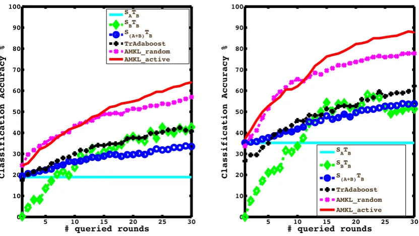
We use several baseline methods to evaluate and compare our transfer
learn-ing results. SATB means we train on source domain Aand test on target domain
B. SBTB means we train on target domain Band test on B. S(A+B)TB means we
train on both A and B and test on B. T rAdaboost means we use the Adaboost
algorithm ([37]) trained on labelled source and target data. AMKL random
means we use adaptive multiple kernel learning and randomly label target
sam-ples. AMKL active (our method) means we use AMKL and actively label the
target samples. For all the experiments, we report the mean accuracy on 5
ran-domly selected train/test sets. SVM parameterC =1 in all the experiments. We
sam-5 10 15 20 25 30 0 10 20 30 40 50 60 70 80 90 100
# queried rounds
Classification Accuracy %
SATB S
BTB S
(A+B)TB TrAdaboost [3] AMKL_random [5] AMKL_active
5 10 15 20 25 30
0 10 20 30 40 50 60 70 80 90 100
# queried rounds
Classification Accuracy %
S ATB S
BTB S(A+B)TB
TrAdaboost [3] AMKL_random [5] AMKL_active
Figure 2.3: Classification accuracies with (left) single view and (right) 4 views.
ple/class) to label every round. To begin with, there are 100 unlabelled images
per class in the target domain.
Fig.2.3 compares classification accuracies achieved using various
ap-proaches over 30 rounds of active learning. Evidently, we can see that our active
transfer learning algorithm outperforms all the considered baselines. Clearly,
our method efficiently learns about the target domain upon incorporating
knowl-edge from a few target examples. Also, employing information from all four
camera views achieves superior performance as compared to monocular
anal-ysis. Comparing AMKL active with AMKL random, we see that in both the
monocular and multi-view cases, our approach outperforms AMKL random
af-ter 10 rounds of AL, and the benefit of learning from the most informative
samples is reflected in the fact that AMKL active outperforms AMKL random
by more than 10% after 30 rounds while classifying with 4-view information.
Fig.2.4 shows the confusion matrix over 24 headpose classes using active
transfer learning after 30 rounds. We can conclude that most of the target
0.82 0.04 0.09 0.01 0.00 0.00 0.00 0.00 0.00 0.00 0.00 0.00 0.03 0.00 0.00 0.00 0.00 0.00 0.00 0.00 0.00 0.00 0.00 0.00 0.12 0.89 0.00 0.00 0.00 0.00 0.00 0.00 0.00 0.00 0.00 0.00 0.00 0.00 0.00 0.00 0.00 0.00 0.00 0.00 0.00 0.00 0.00 0.00 0.01 0.00 0.73 0.00 0.00 0.08 0.00 0.00 0.01 0.00 0.00 0.01 0.00 0.00 0.14 0.00 0.00 0.01 0.00 0.00 0.00 0.00 0.00 0.00 0.01 0.00 0.00 0.68 0.03 0.09 0.02 0.00 0.00 0.00 0.00 0.00 0.00 0.00 0.00 0.00 0.00 0.00 0.00 0.00 0.00 0.00 0.00 0.00 0.00 0.07 0.00 0.16 0.93 0.00 0.00 0.04 0.00 0.00 0.00 0.00 0.00 0.00 0.00 0.00 0.00 0.00 0.00 0.00 0.00 0.00 0.00 0.00 0.00 0.00 0.08 0.11 0.00 0.71 0.00 0.00 0.01 0.00 0.00 0.00 0.00 0.00 0.00 0.00 0.00 0.00 0.00 0.00 0.00 0.00 0.00 0.00 0.00 0.00 0.00 0.03 0.00 0.02 0.79 0.07 0.12 0.08 0.00 0.01 0.00 0.00 0.00 0.00 0.00 0.00 0.00 0.00 0.00 0.00 0.00 0.00 0.00 0.00 0.00 0.01 0.04 0.00 0.08 0.85 0.00 0.00 0.03 0.00 0.00 0.00 0.00 0.00 0.00 0.00 0.00 0.00 0.00 0.00 0.00 0.00 0.00 0.00 0.02 0.00 0.00 0.03 0.08 0.00 0.77 0.00 0.00 0.06 0.00 0.00 0.00 0.00 0.00 0.01 0.00 0.00 0.00 0.00 0.00 0.03 0.00 0.00 0.00 0.00 0.00 0.00 0.01 0.00 0.01 0.78 0.04 0.08 0.00 0.00 0.00 0.00 0.00 0.00 0.00 0.00 0.00 0.05 0.00 0.00 0.00 0.00 0.00 0.00 0.00 0.00 0.00 0.04 0.00 0.04 0.92 0.00 0.00 0.00 0.00 0.00 0.00 0.00 0.00 0.00 0.00 0.00 0.02 0.00 0.00 0.00 0.00 0.00 0.00 0.00 0.01 0.00 0.06 0.09 0.00 0.68 0.00 0.00 0.02 0.00 0.00 0.00 0.00 0.00 0.00 0.01 0.00 0.06 0.04 0.00 0.00 0.00 0.00 0.00 0.00 0.00 0.00 0.00 0.00 0.00 0.59 0.05 0.02 0.01 0.00 0.00 0.00 0.00 0.00 0.00 0.00 0.00 0.00 0.00 0.00 0.00 0.00 0.00 0.00 0.00 0.00 0.00 0.00 0.00 0.20 0.92 0.01 0.01 0.05 0.00 0.00 0.00 0.00 0.00 0.00 0.00 0.00 0.00 0.06 0.00 0.00 0.00 0.00 0.00 0.00 0.00 0.00 0.00 0.08 0.00 0.76 0.03 0.00 0.02 0.00 0.00 0.00 0.00 0.00 0.01 0.00 0.00 0.00 0.00 0.00 0.00 0.00 0.00 0.00 0.00 0.00 0.00 0.09 0.00 0.00 0.66 0.08 0.07 0.03 0.00 0.01 0.00 0.00 0.00 0.00 0.00 0.00 0.00 0.00 0.00 0.00 0.00 0.00 0.00 0.00 0.00 0.01 0.03 0.00 0.05 0.86 0.00 0.00 0.00 0.00 0.00 0.00 0.00 0.00 0.00 0.01 0.00 0.00 0.00 0.00 0.00 0.01 0.00 0.00 0.02 0.00 0.00 0.05 0.18 0.00 0.77 0.03 0.00 0.17 0.00 0.00 0.00 0.00 0.00 0.00 0.00 0.00 0.00 0.01 0.00 0.00 0.00 0.00 0.00 0.00 0.00 0.00 0.06 0.00 0.00 0.81 0.08 0.09 0.05 0.02 0.01 0.00 0.00 0.00 0.00 0.00 0.00 0.00 0.00 0.00 0.00 0.00 0.00 0.00 0.00 0.00 0.00 0.01 0.00 0.06 0.86 0.00 0.00 0.04 0.00 0.00 0.00 0.01 0.00 0.00 0.07 0.00 0.00 0.00 0.00 0.00 0.00 0.00 0.00 0.00 0.00 0.00 0.12 0.04 0.00 0.72 0.00 0.00 0.00 0.00 0.00 0.00 0.00 0.00 0.00 0.00 0.00 0.00 0.01 0.00 0.00 0.00 0.00 0.00 0.00 0.00 0.00 0.03 0.01 0.00 0.73 0.03 0.02 0.00 0.00 0.00 0.00 0.00 0.00 0.00 0.00 0.00 0.00 0.01 0.00 0.00 0.00 0.00 0.00 0.00 0.00 0.00 0.05 0.00 0.03 0.89 0.00 0.00 0.00 0.00 0.00 0.00 0.00 0.00 0.00 0.01 0.00 0.00 0.14 0.00 0.00 0.00 0.00 0.00 0.00 0.00 0.00 0.01 0.13 0.00 0.87
Figure 2.4: Confusion matrix over 24 classes for active DA after 30 rounds.
to nearby classes, which means the samples are only misclassified with respect
to head tilt, while the head pan is classified correctly. This again demonstrates
the robustness of our active DA framework for headpose estimation.
We also evaluate the effects of using five different types of loss function in the
AL module– (i) Logistic loss 1/(1+e2y f(x)), (2) Exponential losse−x, (3) Hinge
loss (1−y)+, (4) Minimum margin loss e−100x and (5) log loss log(1/(1+ x)).
Fig.2.5 presents the active transfer learning classification error obtained on these
different loss function. We observe that hinge loss achieves the better
perfor-mance among all loss functions, which implies that active transfer learning
works optimally if identical loss functions are employed in the DA and AL
modules.
Since querying sample labels for AL can also be done in a batch mode,
we examine the extent of reduction in classification error for varying number
of queried samples at every round. Fig.2.6 shows the progressive reduction
in classification error with differing number of queried samples (4, 8 and 12
samples/class/round) for AL. From Fig.2.6, we can see that the classification
5 10 15 20 25 30 0
0.1 0.2 0.3 0.4 0.5 0.6 0.7 0.8 0.9 1
# queried rounds
Classification Error
logistic loss exponential loss hinge loss minimum margin loss log loss
Figure 2.5: Evaluating active DA classification error with different loss functions.
50 100 150 200 250
0.2 0.25 0.3 0.35 0.4 0.45 0.5 0.55 0.6 0.65 0.7
# queried samples
Classification Error
4 samples per round 8 samples per round 12 samples per round
round. However, choosing a moderate number of queried samples per round
appears to be optimal since the error is minimal when 8 samples per round are
queried as compared to querying 4 or 12 samples per round. Finally, we evaluate
the robustness of our active DA framework to noisy labels. Fig.2.7 compares
classification accuracies achieved with and without modeling for noisy labels
in the AL module (steps 13–19 in Algorithm 1). Note that about 3% higher
accuracy is achieved by accounting for noisy labels when using both monocular
and 4-view image features.
Figure 2.7: Evaluating active domain adaptation with noisy labels modeling strategy.
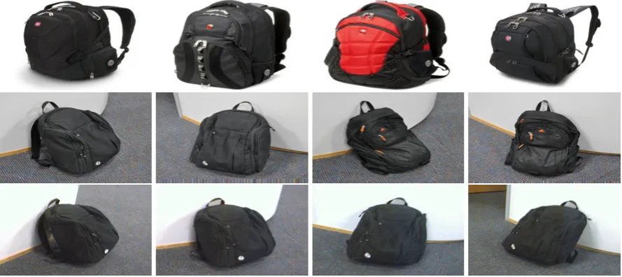
2.4.2 Cross-domain Berkeley Web Image Dataset
The Berkeley image dataset consists of three types of images: web images (from
amazon), images from a digital SLR camera (high resolution image), and
low-resolution webcam images, as shown in Fig.2.8. Each domain has 31 categories
of images. While the digital SLR camera and webcam images capture the same
objects, the viewpoint and image resolutions are different.
Our objective on the Berkeley dataset is to perform object recognition across
Figure 2.8: Exemplars from the Berkeley web image dataset. (from top to bottom) Web (ama-zon), digital SLR camera (high resolution image) and webcam (low resolution image).
5 randomly selected train/test sets. SVM parameter C = 1 in all the
experi-ments. For each object category, there are a small number of labelled samples
in the target domain (3 in our experiment). For the source domain, we use 8
labels per category for webcam/dslr and 20 for amazon. As low-level visual
descriptors, we use the pre-compute SURF features. A codebook of size 800
is constructed by k-means clustering. We firstly normalize the feature vector
and then repeat the experiment as in [84]. Descriptions of the several baseline
methods compared are as follows:
• SATB - We train on source domain Aand test on target domain B.
• SBTB - We train on target domain Band test on B.
• S(A+B)TB - We train on both A and B, and test on B.
• [84] - A metric learning-based DA approach.
• T rAdaboost ([23]) - DA based on the Adaboost algorithm.
• DA - DA with adaptive multiple kernel learning (AMKL) and randomly
• ADA - DA and actively label target samples.
• ADAN - Proposed DA method accounting for noisy labels.
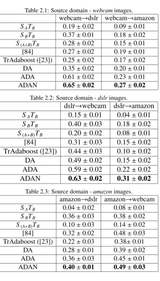
Tables 2.1, 2.2, 2.3 compare classification accuracies achieved with the
dif-ferent approaches when trained on images from the webcam, dslr and amazon
domains respectively. We make the following observations from these tables: (i)
Superior performance is always achieved using SB as compared to SA, which
proves the need for DA for object recognition on the Berkeley dataset. (ii)
While the inductive TrAdaboost and metric learning-based DA approaches
per-form favorably with respect to S(A+B)TB, they are generally outperformed by
the AMKL-based DA approaches studied in this work. (iii) ADA outperforms
DA considerably, implying that AL greatly benefits DA for object recognition.
(iv) ADAN outperforms ADA by up to 5% on an average, implying that our
ap-proach which explicitly accounts for label noise greatly benefits AL. (iv) ADAN
consistently produces the best recognition performance demonstrating the effi
-ciency of the proposed active DA framework.
Commenting on the computational time required for our proposed algorithm,
model training for cross-domain multi-view headpose estimation and object
recognition required 20 minutes with cross-validation on a workstation with
Intel(R) Xeon(R) CPU E5-2620 v2 @ 2.10GHz× 17 processors implying that
our algorithm can be applied on large-scale datasets.
2.5
Conclusion
In this chapter, we propose an active transfer learning framework which
ex-plicitly accounts for ambiguous labels provided by the domain expert. We also
extend traditional active learning for binary classification to a multi-class setting
through error-correcting output coding. Extensive experiments on cross-domain
multi-view head-pose estimation and object recognition demonstrate the eff
Table 2.1: Source domain -webcamimages.
webcam→dslr webcam→amazon
SATB 0.19±0.02 0.09±0.01
SBTB 0.37±0.01 0.18±0.02
S(A+B)TB 0.28±0.02 0.15±0.01
[84] 0.27±0.02 0.19±0.01 TrAdaboost ([23]) 0.25±0.02 0.17±0.02 DA 0.35±0.02 0.20±0.01 ADA 0.61±0.02 0.23±0.01 ADAN 0.65±0.02 0.27±0.02
Table 2.2: Source domain -dslrimages.
dslr→webcam dslr→amazon
SATB 0.15±0.01 0.04±0.01
SBTB 0.40±0.03 0.18±0.02
S(A+B)TB 0.20±0.02 0.08±0.01
[84] 0.31±0.03 0.15±0.02
TrAdaboost ([23]) 0.44±0.03 0.10±0.02
DA 0.49±0.02 0.15±0.02
ADA 0.59±0.02 0.22±0.02
ADAN 0.63±0.02 0.31±0.02
Table 2.3: Source domain -amazonimages.
amazon→dslr amazon→webcam
SATB 0.04±0.02 0.08±0.01 SBTB 0.36±0.03 0.38±0.02
S(A+B)TB 0.10±0.03 0.14±0.02
[84] 0.32±0.02 0.48±0.03
TrAdaboost ([23]) 0.22±0.03 0.38±0.01
DA 0.28±0.01 0.39±0.02
ADA 0.36±0.03 0.45±0.01
informative samples for active learning and handle label noise improves
classi-fication performance with respect to random sample selection.
In the next chapter, we will introduce another learning with shared information
Chapter 3
Multi-task Dictionary Learning
In this chapter, we first propose a novel multi-task dictionary learning
frame-work for the painting style recognition task. Then a novel supervised version of
multi-task dictionary learning is proposed for image recognition.
3.1
Inferring Painting Style with Multi-Task Dictionary
Learning
1Recent advances in imaging and multimedia technologies have paved the way
for automatic analysis of visual art. Despite notable attempts, extracting
rele-vant patterns from paintings is still a challenging task. Different painters, born
in different periods and places, have been influenced by different schools of
arts. However, each individual artist also has a unique signature, which is hard
to detect with algorithms and objective features. In this chapter we propose a
novel dictionary learning approach to automatically uncover the artistic style
from paintings. Specifically, we present a multi-task learning algorithm to learn
a style-specific dictionary representation. Intuitively, our approach, by
auto-matically decoupling style-specific and artist-specific patterns, is expected to
be more accurate for retrieval and recognition tasks than generic methods. To
demonstrate the effectiveness of our approach, we introduce the DART dataset,
containing more than 1.5K images of paintings representative of different styles.
Our extensive experimental evaluation shows that our approach significantly
outperforms state-of-the-art methods.
3.1.1 Introduction
With the continuously growing amount of digitized art available on the web,
classifying paintings into different categories, according to style, artist or based
on the semantic contents, has become essential to properly manage huge
col-lections. In addition, the widespread diffusion of mobile devices has led to an
increased interest in the tourism industry for developing applications that
auto-matically recognize the genre, the art movement, the artist, and the identity of
paintings and provide relevant information to the visitors of museums.
Imaging and multimedia technologies have progressed substantially during
the past decades, encouraging research on automatic analysis of visual art.
Nowadays, art historians have even started to analyse art based on statistical
techniques, e.g. for distinguishing authentic drawings from imitations [47].
However, despite notable attempts [14, 51, 57, 101], the automatic analysis
of paintings is still a complex unsolved task, as it is influenced by many
as-pects,i.e. low-levelfeatures, such as color, texture, shading and stroke patterns,
mid-levelfeatures, such as line styles, geometry and perspective, andhigh-level
features, such as objects presence or scene composition.
In section 3.1 we investigate how to automatically infer the artistic style,i.e.
Baroque, Renaissance, Impressionism, Cubism, Postimpressionism and
Mod-ernism, from paintings. According to Wikipedia, an artistic style is a “tendency
with a specific common philosophy or goal, followed by a group of artists
dur-ing a restricted period of time or, at least, with the heyday of the style defined
within a number of years”. Referring to paintings, the notion of style is more
represen-(1) (2) (3) (4)
(9)
(8) (7)
(10) (5)
(11) (6)
(12)
Figure 3.1: Given the images belonging to theBaroque,Renaissance,Impressionism, Cubism,
Postimpressionism,Modernart movements, can you detect which ones correspond to the same style1?
tative of six art movements are shown, can you guess which ones belong to the
same style? At the first glance, it may not be hard to group these images into
different styles, i.e. (1) and (9), (4) and (8), even if you have never seen these
paintings before. Indeed, human observers can easily match artworks from the
same style and discriminate those originated from different art movements, even
if no a-priori information is provided. That is because humans recognize the
style by implicitly using both low-level cues such as lines or colors and more
subtle compositional patterns.
1Answers: Cubism (1,9), Impressionism (2,7), Postimpressionism (3,10), Renaissance (4,8), Baroque
(6,11), Modern (7,12).
Recently, statistical methods have shown potential for supporting traditional
approaches in the analysis of visual art by providing new, objective and
quan-tifiable measures that assess the artistic style [14, 51, 101]. In this section we
propose a dictionary learning approach for recognizing styles. Dictionary
learn-ing, which has proved to be highly effective in different computer vision and
pattern recognition problems [31, 117], is a class of unsupervised methods for
learning sets of over-complete bases to represent data efficiently. The aim of
dictionary learning is to find a set of basis vectors such that an input vector can
be represented as a linear combination of the basis vectors. In this section we
propose a novel framework unifying multi-task and dictionary learning in order
to simultaneously infer artist-specific and style-specific representations from a
collection of paintings. Our intuition is that if we can build a style-specific
dictionary representation by exploiting common patterns between artists of the
same style with multi-task learning, more accurate results can be obtained for
painting retrieval or recognition. For example, by automatically learning a
dic-tionary for Cubism which captures the features associated to straight lines, we
expect to easily detect that the paintings (1) and (9) in Fig.3.1 belong to the same
category. Our experiments, conducted on the new DART (Dictionary ART)
dataset, confirm our intuition and demonstrate that the learned dictionaries can
be successfully used to recognize the artistic styles.
To summarize, the main contributions of section 3.1 are: (i) We are the first
to introduce the idea of learning style-specific dictionaries for automatic
analy-sis of paintings. (ii) A novel multi-task dictionary learning approach is proposed
through embedding all tasks into an optimal learned subspace. Our multi-task
learning strategy permits to effectively separate artist-specific and style-specific
patterns, improving recognition performances. The proposed machine
learn-ing framework is a generic one and can be easily applied to other problems.
(iii) We collected the DART dataset which contains paintings from different art
movements and different artists.
3.1.2 Related Work
3.1.2.1 Automatic Analysis of Paintings
In literature, [22] were the first to borrow ideas from classification systems for
automatic analysis of visual art and studied the differences between paintings
and photographs. Image features such as edges, spatial variation of colors,
num-ber of unique colors, and pixel saturation were used for classification. [57]
compared van Gogh with his contemporaries by statistical analysis of a
mas-sive set of automatically extracted brushstrokes. [14] introduced the problem
of artistic image annotation and retrieval and proposed several solutions
us-ing graph-based learnus-ing techniques. [101] proposed a SOM-based model for
studying and visualizing the relationships among painting collections of diff
er-ent painters. [123] preser-ented an analysis of the affective cues extracted from
abstract paintings by looking at low-level features and employing a
bag-of-visual-words approach. Few works focused specifically on inferring style from
paintings [51, 86]. However, none of these works have studied the problem of
decoupling artist-specific and style-specific patterns as we do with our
multi-task dictionary learning framework.
3.1.2.2 Dictionary and Multi-task Learning
Dictionary learning has been shown to be able to find succinct representations
of stimuli. Recently, it has been successfully applied to a variety of problems
in computer vision, pattern recognition and image processing, e.g. image
clas-sification [117], denoising [31]. Different optimization algorithms [1, 55] have
also been proposed to solve dictionary learning problems. However, as far as
we know, there is no research work on learning dictionary representations for
recognizing artistic styles.
clas-sification and regression models for a set of related tasks. This is typically
advantageous as compared to considering single tasks separately and not
ex-ploiting their relationships. The goal of multi-task learning is to improve the
performance by learning models for multiple tasks jointly. This works
particu-larly well if these tasks have some commonality while are all slightly
under-sampled. However, there is hardly any work on combining multi-task and
dictionary learning problems. [82] developed an efficient online algorithm for
dictionary learning from multiple consecutive tasks based on the K-SVD
algo-rithm. Another notable exception is [70] where theoretical bounds are provided
to study the generalization error of multi-task dictionary learning algorithms.
[19, 20, 122] proposed different convex formulations for feature selection
prob-lems. These works are very different from ours, since we focus on a specific
applicative scenario and propose a novel multi-task dictionary learning
algo-rithm.
3.1.3 Learning Style-specific Dictionaries
In this section we present our multi-task dictionary learning approach for
in-ferring style-specific representations from paintings. In the following we first
describe the chosen feature descriptors and then the proposed learning
algo-rithm.
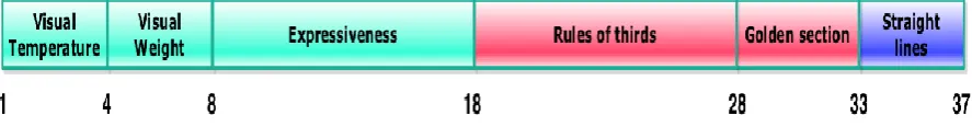
3.1.3.1 Feature Extraction from Paintings
Color, composition and brushstrokes are considered to be the three most
impor-tant components in paintings. Therefore, to represent each painting, we
con-struct a 37-dimensional feature vector as proposed in [101], including color,
composition and lines informations (Fig.3.2).
Color. Following [101], the color features are computed as a function of
lumi-nance and hue. They are: (i) The visual temperature of color (the feel of warmth
con-Figure 3.2: Extracted features: color (light blue), composition (red) and lines (blue).
sidered to be related to the human perception of color temperatures. Different
emotions can be expressed by using cold or warm color temperatures. (ii) The
visual weight of color (the feel of heaviness of color). From the perspective of
psychology, people usually feel that a darker color is heavier and a lighter color
is lighter. (iii) The expressiveness of color (the degree of contrast including
the contrast between luminance, saturation, hue, color temperature, and color
weight). Global and local contrast features are both used to measure the diff
er-ences between pixel and image regions.
Composition. The composition represents the spatial organization of visual
el-ements in a painting. For each image we compute a saliency map. The saliency
map is divided into three parts both horizontally and vertically and we
con-sider the mean salience for each of the nine sections to compute the “rule of
thirds”. Additionally, properties of the most salient region such as size,
elonga-tion, rectangularity and the most salient point are used to represent properties
of ‘golden section’ composition principles. In details, elongation measures the
symmetricity along the principal axes, rectangularity measures how close it is to
its minimum bounding rectangle, the most salient point is the global maximum
of the saliency map.
Lines. Lines in paintings are generally perceived as edges. Different styles of
paintings or different painters may favour a certain type of line. To interpret the
concepts of lines, the Hough Transform is adopted to find straight lines that are
above a certain threshold (longer than 10 pixels). The mean slope, mean length,
Algorithm 2:Learning artist-specific and style-specific dictionaries.
Input:
SamplesX1, ...,Xk fromKtasks
Subspace dimensionalitys, dictionary sizel, regularization parametersλ1,λ2.
Output:
OptimizedP∈Rd×s,Ck ∈Rnk×l,Dk ∈Rl×d,D∈Rl×s.
1: InitializePusing any orthonormal matrix
2: InitializeCkwithl2normalized columns
3: repeat
ComputeDusing Algorithm 2 in [66]
fork=1 : K
ComputeDkusing Algorithm 2 in [66]
ComputeCkusing FISTA [8]
end for
ComputePby eigendecomposition ofB=X0(I−C(C0C)−1C0)X;
untilConvergence;
3.1.3.2 Multi-task Dictionary Learning
Intuitively, in this and in many other applications [52, 67], it is reasonable to
expect that more accurate recognition results are achieved if class specific
dic-tionaries are adopted rather than generic ones. To this end, in this section we
demonstrate that better classification performance are obtained when we
con-sider a style-specific dictionary for each artistic style. In details, we propose
to jointly learn a set of artist-specific dictionaries and discover the underlying
style-specific dictionary projecting data in a low dimensional subspace.
More formally, for each painting style we consider K tasks and the k-th task
corresponds to the k-th artist. Each task consists of data samples denoted by
Xk = [x1k,xk2, ...,xnkk],Xk ∈ IRnk×d,k = 1, ...,K, wherexik ∈ IRd is ad-dimensional
feature vector and nk is the number of samples in the k-th task. We propose
to learn a shared subspace across all tasks, obtained by an orthonormal
projec-tion P ∈ IRd×s, where s is the dimensionality of the subspace. In this learned
subspace, the data distribution from all tasks should be similar to each other.
Therefore, we can code all tasks together in the shared subspace and achieve
individual coding quality by transferring knowledge across all tasks. (ii) We can
discover the relationship among different tasks (artists) via coding analysis. (iii)
The common dictionary among tasks, i.e. the style-specific dictionary, can be
learned by embedding all tasks into a good sharing subspace. These objectives
can be realized solving the optimization problem:
min
Dk,Ck,P,D
K
P
k=1
kXk−CkDkk2F +λ1 K
P
k=1
kCkk1
+λ2 K
P
k=1
kXkP−CkDk2F
s.t.
P0P = I
(Dk)j·(Dk)0j· ≤ 1, ∀j =1, ...,l
Dj·D0j· ≤ 1, ∀j =1, ...,l
(3.1)
where Dk ∈ IRl×d is an over-complete (artist-specific) dictionary (l > d) with l
prototypes of thek-th task, (Dk)j· in the constraints deno