Goodness-of-fit testing for the inverse Gaussian distribution based on new entropy estimation using ranked set sampling and double ranked set sampling

(1)

R E S E A R C H

Open Access

Goodness-of-fit testing for the inverse Gaussian

distribution based on new entropy estimation

using ranked set sampling and double ranked

set sampling

Amer Ibrahim Al-Omari

1*

and Abdul Haq

2

Abstract

Background:

Entropy is a measure of uncertainty and dispersion associated with a random variable. Several

goodness-of-fit tests based on entropy are available in literature and the entropy been widely used in many applications.

Results:

Goodness-of-fit test for the inverse Gaussian distribution is studied based on new entropy estimation using

simple random sampling (SRS), ranked set sampling (RSS) and double ranked set sampling (DRSS) methods. The critical

values of the new tests are obtained using Monte Carlo simulations. The power values of the suggested tests based on

several alternative hypotheses using SRS, RSS, and DRSS are also presented. It is observed that the proposed tests are

more powerful as compared to the test under SRS. Also, it turns out that the test based on DRSS is superior to the RSS

test for all of the cases considered in this study.

Conclusion:

Since the suggested goodness-of-fit tests for the inverse Gaussian distribution using DRSS are more

efficient than that based on RSS, one may consider them using multistage RSS.

Keywords:

Entropy, Goodness-of-fit test, Inverse Gaussian, Root mean square error, Simple random sampling, Ranked set

sampling, Double ranked set sampling

Background

Entropy is a measure of uncertainty and dispersion

asso-ciated with a random variable. It is not uniquely defined,

there exist axiom systems that justify the particular

en-tropies. Shannon (1948) defined the entropy

H

(

f

) of the

random variable

X

as

H f

ð Þ ¼

Z

1

f x

ð Þ

log

f x

ð Þ

dx;

ð

1 Þ

where

X

is a continuous random variable with

prob-ability density function (pdf )

f

(

x

) and cumulative

distribution

function

(cdf )

F

(

x

).

Vasicek

(1976)

defined

H

(

f

) as

H f

ð Þ ¼

Z

1

0

log

d

p

F

1

p

ð Þ

dp:

ð

2 Þ

Let

X1;

X2;

. . .

;

X

n

be a simple random sample of size

n

from

F

(

x

) and let

X

ð Þ1

≤

X

ð Þ2

≤ ⋯ ≤

X

ð Þn

be the order

statistics of the sample. Vasicek (1976) estimator of

_H

(

_f

)

is given by

VE

ðm;nÞ

¼

1 n

X

_n

i¼1

log

n

2 m

X

ðiþmÞ

X

ðimÞ

n

o

;

ð

3 Þ

where

m

is a positive integer, known as a window size,

m

<

n

/2. Here

X

(i)

=

X

(1)

if

i

< 1 and

X

(i)

=

X

(1)

if

i

>

n

. It is of

interest to note that

VE

ðm;nÞ

!

PH f

ð Þ

as

n

!

∞

,

m

!

∞

and

m

/

n

!

0.

* Correspondence:[email protected]

1

Department of Mathematics, Faculty of Science, Al al-Bayt University, Mafraq 25113, Jordan

Full list of author information is available at the end of the article

(2)

Van Es (1992) suggested another entropy estimator

based on spacing's, given by

VE

ðm;nÞ

¼

1 n

m

X

_n_m

i¼1

log

n

þ

1 m

X

ðiþmÞ

X

ð Þi

þ

X

n_k_¼_m

1 k

þ

log

m

n

þ

1 :

ð

4 Þ

They proved the consistency and asymptotic normality

of this estimator under some conditions.

Ebrahimi et al. (1994) suggested a new estimator by

assigning different weights in Vasicek (1976) entropy

es-timator, and proposed the following estimator

EE

ðm;nÞ

¼

1 n

X

n

i¼1

log

n

c

i

m

X

ðiþmÞ

X

ðimÞ

;

ð

5 Þ

where

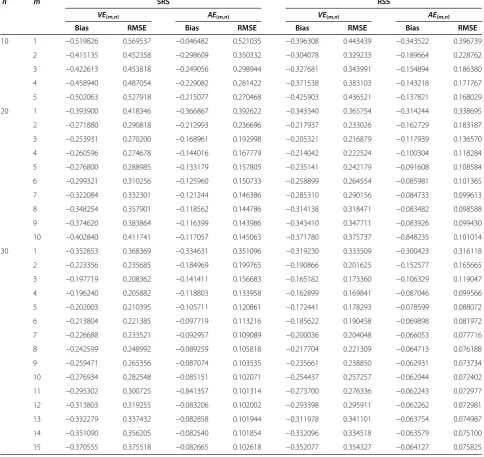
Table 1 Monte Carlo RMSEs and bias values of the entropy estimators

VE

(m,n)

and

AE

(m,n)

for the uniform distribution

,

H

(

f

) = 0

n m SRS RSS

VE(m,n) AE(m,n) VE(m,n) AE(m,n)

Bias RMSE Bias RMSE Bias RMSE Bias RMSE

10 1 −0.519826 0.569537 −0.046482 0.521035 −0.396308 0.443439 −0.343522 0.396739

2 −0.415135 0.452358 −0.298609 0.350332 −0.304078 0.329233 −0.189664 0.228762

3 −0.422613 0.453818 −0.249056 0.298944 −0.327681 0.343991 −0.154894 0.186380

4 −0.458940 0.487054 −0.229082 0.281422 −0.371538 0.383103 −0.143218 0.171767

5 −0.502063 0.527918 −0.215077 0.270468 −0.425903 0.436521 −0.137821 0.168029

20 1 −0.393900 0.418346 −0.366867 0.392622 −0.343340 0.365754 −0.314244 0.338695

2 −0.271880 0.290818 −0.212993 0.236696 −0.217937 0.233026 −0.162729 0.183187

3 −0.253931 0.270200 −0.168961 0.192998 −0.205321 0.216879 −0.117939 0.136570

4 −0.260596 0.274678 −0.144016 0.167779 −0.214042 0.222524 −0.100304 0.118284

5 −0.276800 0.288985 −0.133179 0.157805 −0.235141 0.242179 −0.091608 0.108584

6 −0.299321 0.310256 −0.125960 0.150733 −0.258899 0.264554 −0.085981 0.101365

7 −0.322084 0.332301 −0.121244 0.146386 −0.285310 0.290156 −0.084733 0.099613

8 −0.348254 0.357901 −0.118562 0.144786 −0.314138 0.318471 −0.083482 0.098588

9 −0.374620 0.383864 −0.116399 0.143986 −0.343410 0.347711 −0.083926 0.099430

10 −0.402840 0.411741 −0.117057 0.145063 −0.371780 0.375737 −0.848235 0.101014

30 1 −0.352853 0.368369 −0.334631 0.351096 −0.319230 0.333509 −0.300423 0.316118

2 −0.223356 0.235685 −0.184969 0.199765 −0.190866 0.201625 −0.152577 0.165665

3 −0.197719 0.208362 −0.141411 0.156683 −0.165182 0.173360 −0.106329 0.119047

4 −0.196240 0.205882 −0.118803 0.133958 −0.162899 0.169841 −0.087046 0.099566

5 −0.202003 0.210395 −0.105711 0.120861 −0.172441 0.178293 −0.078599 0.088072

6 −0.213804 0.221385 −0.097719 0.113216 −0.185622 0.190458 −0.069898 0.081972

7 −0.226688 0.233521 −0.092957 0.109089 −0.200036 0.204048 −0.066053 0.077716

8 −0.242599 0.248992 −0.089259 0.105818 −0.217704 0.221309 −0.064713 0.076188

9 −0.259471 0.265356 −0.087074 0.103535 −0.235661 0.238850 −0.062931 0.073734

10 −0.276934 0.282548 −0.085151 0.102071 −0.254437 0.257257 −0.062044 0.072402

11 −0.295302 0.300725 −0.841357 0.101314 −0.273700 0.276336 −0.062243 0.072977

12 −0.313803 0.319255 −0.083206 0.102002 −0.293398 0.295911 −0.062262 0.072981

13 −0.332279 0.337432 −0.082858 0.101944 −0.311978 0.341101 −0.063754 0.074987

14 −0.351090 0.356205 −0.082540 0.101854 −0.332096 0.334518 −0.063579 0.075100

(3)

c

i

¼

1 þ

i

1 m

;

1 ≤

i

≤

m;

2 ;

m

þ

1 ≤

i

≤

n

m;

1 þ

n

i

m

;

n

m

þ

1 ≤

i

≤

n:

8 >

>

<

>

:

Based on the simulation study, it is shown that this

estimator has smaller bias and mean square error

as compared to the Vasicek (1976) entropy estimator.

They proved that

EE

(m,n)

converges in probability to

H

(

f

)

as

n

!

∞

,

m

!

∞

and

m/n

!

0. (Al-Omari AI (2012): Modified entropy estimators

using simple random sampling, ranked set sampling and

double ranked set sampling, Submitted) suggested a

modified estimator of entropy of an unknown

continu-ous pdf

f

(

x

) as

AE

ðm;nÞ

¼

1 n

X

n

i¼1

log

n

c

i

m

X

ðiþmÞ

X

ðimÞ

;

ð

6 Þ

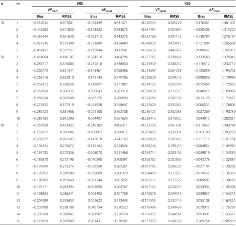
Table 2 Monte Carlo RMSEs and bias values of the entropy estimators

VE

(m,n)

and

AE

(m,n)

for the exponential

distribution,

H

(

f

) = 1

n m SRS RSS

10 1 −0.552032 0.677001 −0.495449 0.631471 −0.430553 0.505229 −0.376361 0.461201

2 −0.442683 0.571820 −0.323532 0.483573 −0.337494 0.404667 −0.220406 0.315220

3 −0.435444 0.561640 −0.265713 0.443276 −0.332760 0.401125 −0.159787 0.276197

4 −0.451545 0.575390 −0.221689 0.424404 −0.348029 0.420617 −0.121584 0.266664

5 −0.469437 0.597761 −0.179844 0.413541 −0.366628 0.445977 −0.080667 0.266812

20 1 −0.414064 0.490107 −0.384516 0.464796 −0.357765 0.398661 −0.333540 0.376843

2 −0.285717 0.376086 −0.232518 0.338830 −0.234959 0.280262 −0.176512 0.232710

3 −0.260773 0.351341 −0.175461 0.298406 −0.213397 0.261261 −0.125059 0.194705

4 −0.256116 0.352810 0.141143 0.279706 −0.210620 0.259248 −0.098056 0.179990

5 −0.262412 0.358638 0.118697 0.271887 −0.214122 0.265246 −0.072456 0.172661

6 −0.265650 0.360325 0.090043 0.263318 −0.218028 0.272315 −0.048075 0.168086

7 −0.266934 0.365008 −0.067175 0.260090 −0.224596 0.282196 −0.023128 0.173677

8 −0.273952 0.377519 −0.041928 0.258647 −0.232629 0.293062 −0.000531 0.176806

9 −0.280123 0.381968 −0.021108 0.262708 −0.236125 0.302083 0.027269 0.190739

10 −0.285183 0.391290 0.004497 0.267634 −0.238413 0.310922 0.044912 0.203657

30 1 −0.367058 0.423423 −0.346283 0.406311 −0.332526 0.361491 −0.313657 0.343784

2 −0.233677 0.306086 −0.198867 0.280012 −0.203455 0.236001 −0.163180 0.203230

3 −0.202277 0.281503 −0.145618 0.241162 −0.170859 0.207468 −0.111717 0.161754

4 −0.194424 0.275072 −0.115163 0.224526 −0.160246 0.199410 −0.084854 0.145930

5 −0.191705 0.272356 −0.095073 0.217468 −0.159714 0.200465 −0.059819 0.134539

6 −0.186870 0.272196 −0.070590 0.208597 −0.158702 0.202869 −0.043778 0.132887

7 −0.191094 0.275374 −0.058550 0.205261 −0.161705 0.206226 −0.027194 0.130283

8 −0.195662 0.280589 −0.036080 0.200329 −0.164468 0.212265 −0.010631 0.136358

9 −0.196983 0.282040 −0.021144 0.202056 −0.165511 0.217222 −0.006685 0.138626

10 −0.197171 0.283394 −0.005890 0.204787 −0.167152 0.220237 0.024904 0.145306

11 −0.198853 0.286241 0.008492 0.207709 −0.173076 0.229318 0.039837 0.154215

12 −0.204089 0.293653 0.022622 0.213445 −0.171555 0.232740 0.055108 0.163320

13 −0.202908 0.298108 0.049154 0.220522 −0.176996 0.240454 0.070977 0.176787

14 −0.205700 0.300842 0.061987 0.226574 −0.176922 0.244541 0.093001 0.193377

(4)

where

c

i

¼

1 þ

1

2 ;

1 ≤

i

≤

m;

2 ;

m

þ

1 ≤

i

≤

n

m;

1 þ

1

2 ;

n

m

þ

1 ≤

i

≤

n:

8 >

>

<

>

:

Alizadeh (2010) proposed a new estimator of entropy

and studied its application in testing normality. Park and

Park (2003) considered correcting moments for

goodness-of-fit tests for two entropy estimates.

Inverse Gaussian distribution

A random variable

X

is said to have an inverse Gaussian

distribution function

IG

(

x

;

μ

,

β

), if its pdf is of the

fol-lowing form

f x

ð Þ ¼

ffiffiffiffiffiffiffiffiffiffi

β

2 π

x

3

r

exp

β

2 μ

2

_x

ð

x

μ

Þ

2

;

for

x

>

0 ;

ð

7 Þ

where

μ

>

0 is the mean and

β

>

0 is the shape parameter.

The variance of

X

is

μ

3

β

. Its characteristic function is

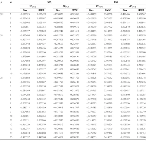
VE

(m,n)

AE

(m,n)

distribution,

H

(

f

) = 1.419

n m SRS RSS

10 1 −0.598925 0.676499 −0.538428 0.623068 −0.484489 0.549750 −0.429406 0.502967

2 −0.521455 0.591007 −0.409842 0.496627 −0.422169 0.471157 −0.308706 0.375690

3 −0.563002 0.623188 −0.386562 0.468471 −0.462240 0.504378 −0.291133 0.353844

4 −0.610651 0.663364 0.388846 0.469519 −0.523019 0.557792 −0.292810 0.351636

5 −0.671777 0.719069 −0.382242 0.461612 −0.584483 0.614209 −0.294820 0.349472

20 1 −0.435480 0.483459 −0.402721 0.452976 −0.382986 0.420310 −0.354315 0.393878

2 −0.327145 0.375798 −0.267005 0.324501 −0.275716 0.313472 −0.218758 0.264068

3 −0.317948 0.364927 −0.230598 0.292997 −0.268657 0.304811 −0.181588 0.230636

4 −0.327070 0.372436 −0.214227 0.279269 −0.285331 0.318855 −0.168035 0.219922

5 −0.352658 0.395796 −0.205782 0.272804 −0.305555 0.337744 −0.160392 0.213700

6 0.375996 0.416964 −0.203268 0.269194 −0.335066 0.365185 −0.162263 0.216405

7 −0.404050 0.442997 −0.200951 0.269828 −0.363782 0.391748 −0.162648 0.217866

8 −0.439618 0.475094 −0.203704 0.270603 −0.395221 0.421583 −0.163443 0.217711

9 −0.467134 0.500777 0.211872 0.276695 −0.428042 0.451680 −0.169841 0.224475

10 −0.496926 0.527456 −0.209085 0.275281 −0.454818 0.477152 −0.171572 0.224804

30 1 −0.378860 0.413455 −0.359097 0.394766 −0.343626 0.370512 −0.328056 0.355718

2 −0.259105 0.299687 −0.221750 0.266138 −0.226914 0.255947 −0.189446 0.223276

3 −0.236758 0.277238 −0.177599 0.229027 −0.204698 0.234358 −0.147274 0.186797

4 −0.234369 0.275867 −0.158560 0.213972 −0.204765 0.234413 −0.125487 0.169031

5 −0.244288 0.283027 −0.148610 0.206988 −0.214434 0.243683 −0.117590 0.165087

6 −0.255248 0.293332 −0.139542 0.200072 −0.227340 0.255901 −0.111407 0.161770

7 −0.269724 0.305134 −0.132038 0.196792 −0.241325 0.268228 −0.105796 0.158654

8 −0.285713 0.321039 −0.129915 0.193509 −0.254983 0.282376 −0.102504 0.157726

9 −0.304064 0.337563 −0.131105 0.198239 −0.274697 0.301420 −0.103392 0.160749

10 −0.320051 0.352764 −0.130086 0.196928 −0.295057 0.319933 −0.101392 0.160593

11 −0.339131 0.369866 −0.127890 0.196985 −0.314201 0.339141 −0.102034 0.161378

12 −0.361226 0.392070 −0.130212 0.197655 −0.333173 0.356224 −0.103026 0.163577

13 −0.382347 0.410463 0.129885 0.199488 −0.353582 0.375170 −0.105978 0.165825

14 −0.400618 0.428008 −0.131518 0.199794 −0.375752 0.397462 −0.109190 0.168154

(5)

given by

ϕ

_x

ð Þ ¼

t

exp

β

_μ

p

ffiffiffi

β

ffiffiffiffiffiffiffiffiffiffiffiffiffiffiffiffi

β

μ

2

2 it

s

!

:

The

IG

(

x

;

μ

,

β

) has many applications in the field,

for example see Seshadri (1999), and Folks and

Chhikara (1998).

Method

The test procedure

Let

X1;

X2;

. . .

;

X

n

be a random sample of size

n

drawn

from the pdf

f

(

x

) and let

X

ð Þ1

≤

X

ð Þ2

≤ ⋯ ≤

X

ð Þn

be the

order statistics of this sample. Our interest is to test that

this random sample is coming from an inverse Gaussian

population or not. Thus, the composite null hypothesis

is

H

0

:

X

~

IG

(

x

;

μ

,

β

).

The following corollary is due to Mahdizaheh and

Arghami (2010).

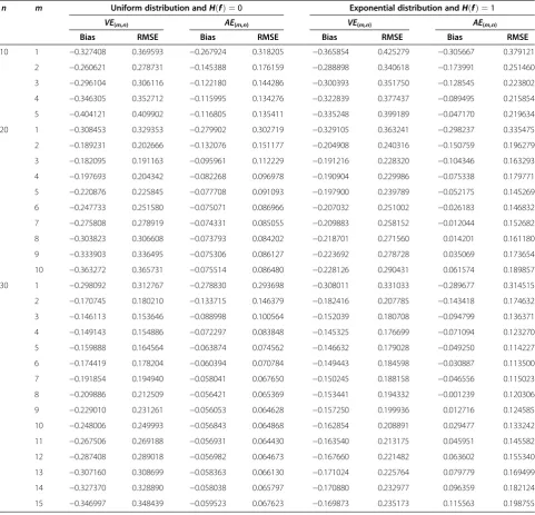
Table 4 Monte Carlo RMSEs and bias values of the entropy estimators

VE

(m,n)

and

AE

(m,n)

for the uniform distribution

with

H

(

f

) = 0 and exponential distribution with

H

(

f

) = 1 using DRSS

n m Uniform distribution and_{H f}_{ð Þ ¼}0 Exponential distribution and_{H f}_{ð Þ ¼}1

10 1 −0.327408 0.369593 −0.267924 0.318205 −0.365854 0.425279 −0.305667 0.379121

2 −0.260621 0.278731 −0.145388 0.176159 −0.288898 0.340618 −0.173991 0.251460

3 −0.296104 0.306116 −0.122180 0.144286 −0.300393 0.351750 −0.128545 0.223802

4 −0.346305 0.352712 −0.115995 0.134276 −0.322839 0.377437 −0.089495 0.215854

5 −0.404121 0.409902 −0.116805 0.135411 −0.335248 0.399189 −0.047170 0.219634

20 1 −0.308453 0.329353 −0.279902 0.302719 −0.329105 0.363241 −0.298237 0.335475

2 −0.189231 0.202666 −0.132076 0.151177 −0.204908 0.240316 −0.150759 0.196279

3 −0.182095 0.191163 −0.095961 0.112229 −0.191216 0.228320 −0.104346 0.163293

4 −0.197693 0.204342 −0.082268 0.096978 −0.190904 0.229986 −0.075338 0.179771

5 −0.220876 0.225845 −0.077708 0.091093 −0.197900 0.239789 −0.052175 0.145269

6 −0.247733 0.251580 −0.075071 0.086966 −0.207032 0.251002 −0.026183 0.146832

7 −0.275808 0.278919 −0.074331 0.085055 −0.209883 0.258152 −0.012044 0.152682

8 −0.303823 0.306608 −0.073793 0.084202 −0.218701 0.271560 0.014201 0.161180

9 −0.333903 0.336495 −0.075306 0.086127 −0.223692 0.278728 0.035069 0.173654

10 −0.363272 0.365731 −0.075514 0.086480 −0.228126 0.290431 0.061574 0.189857

30 1 −0.298092 0.312767 −0.278830 0.293698 −0.308011 0.331033 −0.289677 0.314515

2 −0.170745 0.180210 −0.133715 0.146379 −0.182416 0.207785 −0.143418 0.174632

3 −0.146113 0.153646 −0.088998 0.100564 −0.152039 0.180708 −0.094799 0.136371

4 −0.149143 0.154886 −0.072297 0.083848 −0.145325 0.176699 −0.071094 0.123270

5 −0.159888 0.164564 −0.063874 0.074562 −0.146632 0.179028 −0.049250 0.114227

6 −0.174419 0.178204 −0.060394 0.070784 −0.149443 0.184598 −0.030887 0.113500

7 −0.191854 0.194940 −0.058041 0.067650 −0.150245 0.188158 −0.046556 0.115023

8 −0.209886 0.212509 −0.056421 0.065369 −0.153441 0.194332 −0.001239 0.120306

9 −0.229010 0.231261 −0.056053 0.064628 −0.157250 0.199936 0.012716 0.124585

10 −0.248006 0.249993 −0.056843 0.064868 −0.162854 0.208891 0.029477 0.133242

11 −0.267506 0.269188 −0.056931 0.064430 −0.163540 0.213175 0.045951 0.145582

12 −0.287408 0.289018 −0.056982 0.064673 −0.167660 0.221482 0.063602 0.155340

13 −0.307160 0.308699 −0.058363 0.066130 −0.171024 0.225764 0.079779 0.169499

14 −0.327370 0.328890 −0.058038 0.065797 −0.170880 0.232977 0.096359 0.182124

(6)

Corollary 1

: Assume that

X

is a random variable has

an inverse Gaussian distribution

IG

(

x

;

μ

,

β

) and let

Y

¼

1 =

p

ffiffiffiffi

X

Then the entropy of

Y

is given by

H f y

ð

ð Þ

Þ ¼

log 0

:

5 ϕ

p

ffiffiffiffiffiffiffiffi

2 π

e

, where

ϕ

2

_¼

₁

₌

_β

_¼

_{E Y}

_{ð Þ}

2

₁

_{=E Y}

_ð

2

_Þ

_:

The following corollary is due to Mudholkar and Tian

(2002).

Corollary 2

: The random variable

X

with inverse

Gaussian distribution

IG

(

x

;

μ

,

β

) is characterized by the

property that

1 =

p

ffiffiffiffi

X

attains the maximum entropy

among all nonnegative, absolutely continuous random

variables

Y

with a given value at

E Y

_{ð Þ}

2

₁

_{=E Y}

_ð

2

_Þ

_:

Let

VE

ðm;nÞ

f

y

be the sample estimate of

VE f

y

for

the distribution of

Y

¼

1 =

p

ffiffiffiffi

X

defined as

VE

ðm;nÞ

f

y

¼

1 n

X

_n

i¼1

Log

n

2 m

y

ðiþmÞ

y

ðimÞ

;

ð

8 Þ

where

y

ð Þi

¼

x

ðniþ1Þ

1=2

i

¼

1 ;

2 ;

. . .

;

n

ð

Þ

:

Mahdizaheh and Arghami (2010) followed Vasicek

(1976) and proposed rejecting the null hypothesis

H

0

:

X

~

IG

(

x

;

μ

,

β

) if

K

ðm;nÞ

f

y

¼

2 exp VE

ðm;nÞ

f

y

ψ

≤

K

ðm;n;αÞ

f

y

;

ð

9 Þ

where

ψ

2

is a uniform minimum variance unbiased

(UMVU) estimate of

Ø

2

defined as

ψ

2

_¼

1 n

1 X

1 =x

_i

1 =

x

ð

Þ

¼

1 n

¼

1 X

n

i¼1

y

2

i

n

2

X

n

i¼1

yi

2

1

:

ð

10 Þ

Suggested test

Let

X

i(i)

denote the

i

th order statistic from the

i

th

sam-ple

ð

i

¼

1 ;

2 ;

. . .

;

n

Þ

. Then, the measured RSS units are

denoted by

X

1(1)

,

X

2(2)

,

. . .,

X

n(n)

. The cumulative

distri-bution function of

X

i(i)

is given by

F

ð Þi

ð Þ ¼

x

X

_n

j¼i

n

j

F

j

_{ð Þ}

_x

_ð

₁

_{F x}

_{ð Þ}

_Þ

nj

_;

₁

_<

x

<

1 ;

with probability density function defined as

f

ð Þi

ð Þ ¼

x

n

_i

₁

1 F

i1

_{ð Þ}

_x

_ð

₁

_{F x}

_{ð Þ}

_Þ

ni

_{f x}

_{ð Þ}

_;

₁

_<

_x

<

1 :

The mean and the variance of the

i

th order statistic,

X

i(i)

can be written respectively as

μ

ð Þ ¼

i

Z

1

xf

ð Þi

ð Þ

x

d

x;

and

σ

2

i ð Þ

¼

Z

1

x

μ

ð Þi

2

f

ð Þi

ð Þ

x

d

x:

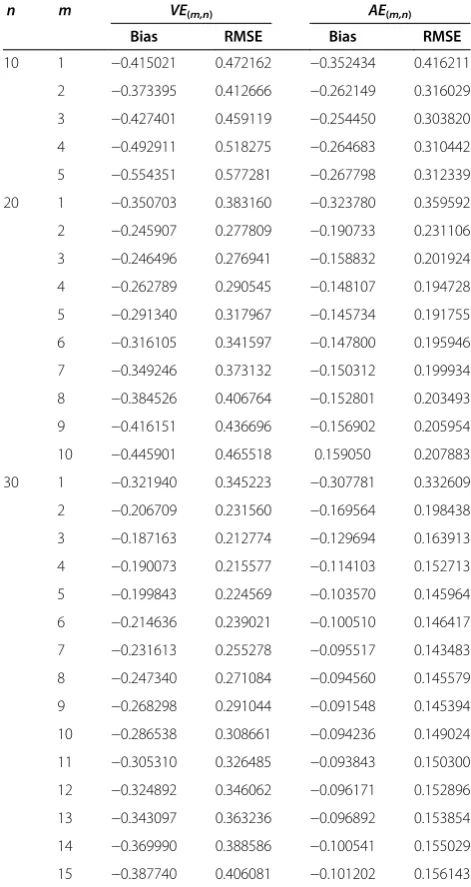
entropy estimators

VE

(m,n)

and

AE

(m,n)

for the standard

normal distribution and

H

(

f

) = 1.419 using DRSS

n m VE(m,n) AE(m,n)

Bias RMSE Bias RMSE

10 1 ₋0.415021 0.472162 ₋0.352434 0.416211

2 ₋0.373395 0.412666 ₋0.262149 0.316029

3 ₋0.427401 0.459119 ₋0.254450 0.303820

4 ₋0.492911 0.518275 ₋0.264683 0.310442

5 ₋0.554351 0.577281 ₋0.267798 0.312339

20 1 ₋0.350703 0.383160 ₋0.323780 0.359592

2 ₋0.245907 0.277809 ₋0.190733 0.231106

3 ₋0.246496 0.276941 ₋0.158832 0.201924

4 ₋0.262789 0.290545 ₋0.148107 0.194728

5 ₋0.291340 0.317967 ₋0.145734 0.191755

6 ₋0.316105 0.341597 ₋0.147800 0.195946

7 −0.349246 0.373132 −0.150312 0.199934

8 −0.384526 0.406764 −0.152801 0.203493

9 −0.416151 0.436696 −0.156902 0.205954

10 −0.445901 0.465518 0.159050 0.207883

30 1 ₋0.321940 0.345223 ₋0.307781 0.332609

2 ₋0.206709 0.231560 ₋0.169564 0.198438

3 ₋0.187163 0.212774 ₋0.129694 0.163913

4 ₋0.190073 0.215577 ₋0.114103 0.152713

5 ₋0.199843 0.224569 ₋0.103570 0.145964

6 ₋0.214636 0.239021 ₋0.100510 0.146417

7 ₋0.231613 0.255278 ₋0.095517 0.143483

8 ₋0.247340 0.271084 ₋0.094560 0.145579

9 ₋0.268298 0.291044 ₋0.091548 0.145394

10 ₋0.286538 0.308661 ₋0.094236 0.149024

11 ₋0.305310 0.326485 ₋0.093843 0.150300

12 ₋0.324892 0.346062 ₋0.096171 0.152896

13 ₋0.343097 0.363236 ₋0.096892 0.153854

14 ₋0.369990 0.388586 ₋0.100541 0.155029

15 −0.387740 0.406081 −0.101202 0.156143

(7)

The ranked set sampling method was suggested by

McIntyre (1952) for estimating the mean of pasture and

forage yields. The RSS can be described as follows:

Step 1: Select

n

simple random samples each of size

n

from the target population.

Step 2: Without cost, visually rank the units within

each sample with respect to the variable of interest.

Step 3: For actual measurement, from the

i

th

i

¼

1 ;

2 ;

. . .

;

n

ð

Þ

sample of

n

units, select the

i

th smallest

ranked unit. The method is repeated

h

times if needed

to increase the sample size to

hn

units.

Al-Saleh and Al-Kadiri (2000) suggested double ranked

set sampling (DRSS) method for estimating the population

mean. The DRSS can be described as in the following steps:

Step 1 Randomly select

n

2

samples each of size

n

from

the target population.

Step 2 Apply the RSS method on the

n

2

samples obtained

in Step 1. This step yields

n

samples each of size

n

.

Step 3 Reapply the RSS method again on the

n

sam-ples obtained on Step 2 to obtain a sample of size

n

from the DRSS data. The cycle can be repeated

h

times

if needed to obtain a sample of size

hn

units.

The SRS estimator of the population mean is given by

^

μ

_SRS

¼

X

n_i_¼₁

X

i

=n;

with variance

Var

ð

^

μ

SRS

Þ ¼

σ

2

=n

. The

RSS estimator of the population mean is defined as

^

μ

_RSS

¼

X

n_i_¼₁

X

i ið Þ

=n

, with variance given by

Var

ð

^

μ

RSS

Þ ¼

σ2

n

n12

X

n

i¼1

μ

ð Þi

μ

2

. The relative precision (RP) of

RSS relative to SRS for estimating the population mean

is

RP

¼

Var

μ

SRS

Var

μ

RSS

¼

1 i

¼

1 n

μ

i

μ

2 n

σ

2

:

Takahasi and Wakimoto (1968) showed that the parent

pdf

f

(

x

) and the population mean can be expressed as

f x

ð Þ ¼

1

n

X

_n

i¼1

f

ð Þi

ð Þ

x

;

and

μ

¼

1

n

X

_n

i¼1

μ

ð Þi

, respectively.

Also, they showed that 1

≤

RP

≤

mþ1

2

, where the lower

bound is attained if and only if the underlying

distribu-tion is degenerate, while the upper bound is attained if

and only if the underlying distribution of the data is

rectangular.

Al-Saleh and Al-Omari (2002) extended the DRSS for

multistage RSS method to increase the efficiency of the

estimators for fixed value of the sample size, Al-Omari

and Raqab (2012) suggested truncation RSS method for

estimating the population mean and median, Al-Omari

(2011) suggested double robust extreme RSS for

estimat-ing the population mean, Haq and Shabbir (2010)

pro-posed a family of ratio estimators of the population

mean using extreme RSS based on two auxiliary

variables.

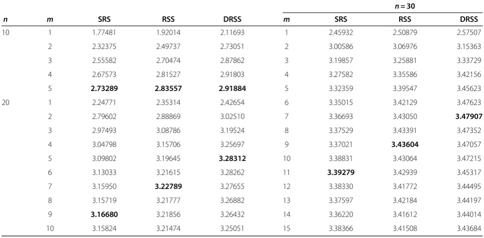
Table 6 Critical values of the test statistics at significance level

α

= 0.05 using SRS, RSS and DRSS

n= 30

n m SRS RSS DRSS m SRS RSS DRSS

10 1 1.77481 1.92014 2.11693 1 2.45932 2.50879 2.57507

2 2.32375 2.49737 2.73051 2 3.00586 3.06976 3.15363

3 2.55582 2.70474 2.87862 3 3.19857 3.25881 3.33729

4 2.67573 2.81527 2.91803 4 3.27582 3.35586 3.42156

5 2.73289 2.83557 2.91884 5 3.32359 3.39547 3.45623

20 1 2.24771 2.35314 2.42654 6 3.35015 3.42129 3.47623

2 2.79602 2.88869 3.02510 7 3.36693 3.43050 3.47907

3 2.97493 3.08786 3.19524 8 3.37529 3.43391 3.47352

4 3.04798 3.15706 3.25697 9 3.37021 3.43604 3.47057

5 3.09802 3.19645 3.28312 10 3.38831 3.43064 3.47215

6 3.13033 3.21615 3.28262 11 3.39279 3.42939 3.45317

7 3.15950 3.22789 3.27655 12 3.38330 3.41772 3.44495

8 3.15719 3.21777 3.26882 13 3.37597 3.42184 3.44197

9 3.16680 3.21856 3.26432 14 3.36220 3.41612 3.44014

10 3.15824 3.21474 3.25051 15 3.38366 3.41508 3.43684

Table 7 Optimal window sizes

n SRS RSS DRSS

10 5 5 5

20 9 7 5

(8)

Goodness-of-fit test for the

IG

(

x

;

μ

,

β

) distribution is

considered using SRS, RSS and DRSS methods. Our

composite null hypothesis is

H

0

:

X

~

IG

(

x

;

μ

,

β

).

Follow-ing Mudholkar and Tian (2002), we reject

H

0

if

K

ðm;nÞ

f

y

¼

2 exp

AE

ðm;nÞ

f

y

ψ

≤

K

ðm;n;αÞ

f

y

;

ð

11 Þ

where

AE

ðm;nÞ

¼

n1

X

n

i¼1

Log

n

c

i

m

X

ðiþmÞ

X

ðimÞ

and

c

i

¼

1 þ

1

2 ;

1 ≤

i

≤

m;

2 ;

m

þ

1 ≤

i

≤

n

m;

1 þ

1

2 ;

n

m

þ

1 ≤

i

≤

n:

8 >

>

<

>

:

Note that,

AE

ðm;nÞ

f

y

is the sample estimate of

AE f

y

.

Since the entropy estimators are functions of order

sta-tistics, then the entropy estimation using RSS and DRSS

involves ordering the RSS units.

Results and discussion

In this section, a Monte Carlo experiment is presented to

investigate the performance of the entropy estimators i.e.

AE

(m,n)

as well as

VE

(m,n)

and as well as to study the

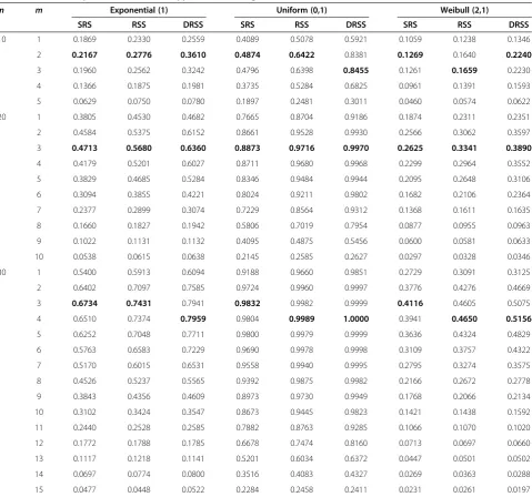
α

n m Exponential (1) Uniform (0,1) Weibull (2,1)

SRS RSS DRSS SRS RSS DRSS SRS RSS DRSS

10 1 0.1869 0.2330 0.2559 0.4089 0.5078 0.5921 0.1059 0.1238 0.1346

2 0.2167 0.2776 0.3610 0.4874 0.6422 0.8381 0.1269 0.1640 0.2240

3 0.1960 0.2562 0.3242 0.4796 0.6398 0.8455 0.1261 0.1659 0.2230

4 0.1366 0.1875 0.1981 0.3735 0.5284 0.6825 0.0961 0.1391 0.1593

5 0.0629 0.0750 0.0780 0.1897 0.2481 0.3011 0.0460 0.0574 0.0622

20 1 0.3805 0.4530 0.4682 0.7665 0.8704 0.9186 0.1874 0.2311 0.2351

2 0.4584 0.5375 0.6152 0.8661 0.9528 0.9930 0.2566 0.3062 0.3597

3 0.4713 0.5680 0.6360 0.8873 0.9716 0.9970 0.2625 0.3341 0.3890

4 0.4179 0.5201 0.6027 0.8711 0.9680 0.9968 0.2299 0.2964 0.3552

5 0.3829 0.4685 0.5284 0.8346 0.9484 0.9944 0.2095 0.2648 0.3106

6 0.3094 0.3855 0.4221 0.8024 0.9211 0.9802 0.1682 0.2106 0.2364

7 0.2377 0.2899 0.3074 0.7229 0.8564 0.9312 0.1368 0.1611 0.1635

8 0.1660 0.1827 0.1942 0.5806 0.7019 0.7954 0.0877 0.0955 0.0963

9 0.1022 0.1131 0.1132 0.4095 0.4875 0.5456 0.0600 0.0581 0.0633

10 0.0538 0.0615 0.0638 0.2145 0.2585 0.2627 0.0297 0.0328 0.0346

30 1 0.5400 0.5913 0.6094 0.9188 0.9660 0.9851 0.2729 0.3091 0.3125

2 0.6402 0.7097 0.7585 0.9724 0.9960 0.9997 0.3776 0.4276 0.4669

3 0.6734 0.7431 0.7941 0.9832 0.9982 0.9999 0.4116 0.4605 0.5075

4 0.6510 0.7374 0.7959 0.9804 0.9989 1.0000 0.3941 0.4650 0.5156

5 0.6252 0.7048 0.7711 0.9800 0.9979 0.9999 0.3636 0.4324 0.4829

6 0.5763 0.6583 0.7229 0.9690 0.9978 0.9998 0.3109 0.3757 0.4322

7 0.5170 0.6015 0.6531 0.9558 0.9940 0.9995 0.2795 0.3274 0.3575

8 0.4526 0.5237 0.5565 0.9392 0.9875 0.9982 0.2166 0.2672 0.2778

9 0.3843 0.4356 0.4609 0.8973 0.9730 0.9949 0.1768 0.2066 0.2134

10 0.3102 0.3424 0.3547 0.8673 0.9445 0.9823 0.1421 0.1438 0.1592

11 0.2440 0.2528 0.2585 0.7882 0.8763 0.9285 0.1066 0.1070 0.1020

12 0.1772 0.1788 0.1785 0.6678 0.7474 0.8160 0.0713 0.0697 0.0660

13 0.1117 0.1218 0.1141 0.5201 0.6034 0.6372 0.0447 0.0501 0.0502

14 0.0697 0.0774 0.0800 0.3516 0.4083 0.4327 0.0269 0.0363 0.0288

(9)

powers of the suggested tests under different alternatives

hypotheses. The root mean square errors (RMSEs) and

the bias values are obtained for the estimators based on

10,000 samples of sizes

n

= 10, 20, 30 with window sizes

1 ≤

m

≤

5, 1

≤

m

≤

10 and 1

≤

m

≤

15, respectively.

Comparison between

VE(

m,n)

and

AE(

m,n)

The samples are selected from the uniform, exponential

and the standard normal distributions using SRS, RSS and

DRSS methods. From Tables 1, 2, 3, 4, 5, 6, and 7 we can

see that

AE

ðm;nÞ

is more efficient than

VE

ðm;nÞ

for all cases

considered in this study. Also, the DRSS is superior to

SRS and RSS. For more details about this comparison

see (Al-Omari AI (2012): Modified entropy estimators

using simple random sampling, ranked set sampling

and double ranked set sampling, Submitted).

We can see that these optimal values are different from

Mahdizaheh and Arghami (2010) values where their

sug-gested test is based on Vasicek (1976) entropy estimator.

Here, we can conclude that the optimal window size

depends on the entropy estimator used for the

goodness-of-fit test.

Power of the tests

The power of the suggested goodness-of-fit tests using SRS,

RSS and DRSS is considered here relative to the same

alter-natives considered by Mahdizaheh and Arghami (2010) for

the distributions, exponential(1), uniform(0,1), Weibull(2,1),

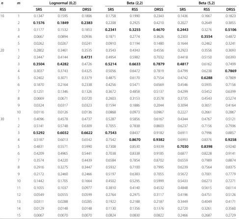
Table 9 Power comparison for the entropy tests at the significance level

α

= 0.05

n m Lognormal (0,2) Beta (2,2) Beta (5,2)

SRS RSS DRSS SRS RSS DRSS SRS RSS DRSS

10 1 0.1347 0.1595 0.1806 0.1758 0.1990 0.2343 0.1436 0.1667 0.1823

2 0.1576 0.1849 0.2383 0.2208 0.2925 0.4210 0.2027 0.2649 0.3855

3 0.1177 0.1532 0.1853 0.2341 0.3255 0.4670 0.2443 0.3276 0.5106

4 0.0667 0.0894 0.0936 0.1871 0.2774 0.3626 0.2303 0.3554 0.4872

5 0.0262 0.0267 0.0241 0.0910 0.1194 0.1480 0.1644 0.2462 0.3241

20 1 0.2802 0.3461 0.3535 0.3543 0.4343 0.4556 0.2923 0.3556 0.3693

2 0.3447 0.4144 0.4731 0.4954 0.5982 0.7032 0.4418 0.5150 0.6393

3 0.3504 0.4282 0.4726 0.5214 0.6633 0.7879 0.4817 0.6162 0.7499

4 0.3037 0.3743 0.4325 0.5056 0.6472 0.7819 0.4799 0.6238 0.7869

5 0.2402 0.3071 0.3379 0.4875 0.6170 0.7554 0.4742 0.6288 0.7809

6 0.1870 0.2164 0.2338 0.4256 0.5471 0.6569 0.4546 0.5935 0.7156

7 0.1251 0.1346 0.1326 0.3672 0.4858 0.5137 0.4299 0.5452 0.6399

8 0.0669 0.0671 0.0720 0.2603 0.3153 0.3578 0.3735 0.4543 0.5274

9 0.0324 0.0317 0.0323 0.1594 0.1886 0.2044 0.3094 0.3651 0.4164

10 0.0116 0.0126 0.0136 0.0868 0.0973 0.0967 0.2227 0.2661 0.2867

30 1 0.4096 0.4578 0.4737 0.5287 0.5856 0.6167 0.4344 0.4767 0.5121

2 0.5141 0.5748 0.6309 0.7055 0.7838 0.8603 0.6237 0.7156 0.7936

3 0.5292 0.6032 0.6622 0.7543 0.8437 0.9182 0.6911 0.7996 0.8857

4 0.5187 0.6013 0.6542 0.7542 0.8670 0.9382 0.6993 0.8376 0.9258

5 0.4831 0.5571 0.5990 0.7308 0.8530 0.9339 0.7030 0.8398 0.9240

6 0.4209 0.4965 0.5441 0.7038 0.8338 0.9185 0.6877 0.8228 0.9141

7 0.3574 0.4220 0.4439 0.6584 0.7854 0.8702 0.6559 0.7989 0.8874

8 0.2916 0.3275 0.3447 0.5932 0.7100 0.7995 0.6239 0.7564 0.8375

9 0.2172 0.2460 0.2466 0.5197 0.6383 0.7055 0.5672 0.7001 0.7779

10 0.1442 0.1705 0.1664 0.4502 0.5295 0.5999 0.5433 0.6273 0.7271

11 0.1055 0.1037 0.0977 0.3810 0.4140 0.4532 0.4848 0.5615 0.6114

12 0.0549 0.0555 0.0599 0.2764 0.2975 0.3117 0.4196 0.4751 0.5126

13 0.0311 0.0288 0.0285 0.1922 0.2188 0.2187 0.3449 0.4049 0.4171

14 0.0129 0.0148 0.0148 0.1130 0.1356 0.1376 0.2720 0.3261 0.3560

(10)

lognormal(0,2), beta(2,2), and beta(5,2). 10000 samples of

sizes

n

= 30, 20, 30 are generated for each method at the

significance level 0.05.

Based on Tables 8 and 9, we can conclude that gain in

the performance of the new suggested tests using

differ-ent methods considered in this paper is obtained.

How-ever, we found that the DRSS is superior to both RSS

and SRS methods based on the sample size. Also, the

RSS performs better than SRS for all cases considered

here. The bold fonts in Tables 8 and 9 are the optimal

power values for each design with the same sample size.

These optimal power values are

<

n=

2. However, the

op-timal values of the window size are 2, 3, 4, 5. For fixed

n

,

the power values decreases as

m

increases, while it

increases in

n.

Conclusion

In this paper, new goodness-of-fit tests for the inverse

Gaussian distribution are suggested using SRS, RSS and

DRSS based on the maximum entropy characterization.

It is found that the new tests are more powerful under

RSS and DRSS, and the test under DRSS is superior to

the tests under RSS and SRS methods. We recommend

using the suggested goodness-of-fit tests for the inverse

Gaussian distribution. As the DRSS is better than RSS,

the current work can be extended to multistage RSS

de-sign and for some other probability distributions.

Competing interests

Both authors declared that they have no competing.

Authors’contribution

The work presented here was carried out in collaboration between authors. AA carried out the theoretical and discussion of this paper. AH carried out the Monte Carlo simulations. All authors read and approved the final manuscript.

Acknowledgment

The authors are grateful to the editors and the anonymous reviewers for their valuable comments and suggestions.

Author details

1_{Department of Mathematics, Faculty of Science, Al al-Bayt University, Mafraq} 25113, Jordan.2Department of Statistics, Quaid-i-Azam University, Islamabad 45320, Pakistan.

Received: 26 July 2012 Accepted: 29 August 2012 Published: 15 September 2012

References

Alizadeh HN (2010) A new estimator of entropy and its application in testing normality. J Stat Comput Simul 80:1151–1162

Al-Omari AI (2011) Estimation of mean based on modified robust extreme ranked set sampling. J Stat Comput Simul 81(8):1055–1066

Al-Omari AI, Raqab MZ (2012) Estimation of the population mean and median using truncation-based ranked set samples. Accepted in J Stat Comput Simul. doi:10.1080/00949655.2012.662684

Al-Saleh MF, Al-Kadiri MA (2000) Double ranked set sampling. Stat probability lett 48(2):205–212

Al-Saleh MF, Al-Omari AI (2002) Multistage ranked set sampling. J Stat Planning and Inference 102(2):273–286

Ebrahimi N, Pflughoeft K, Soofi E (1994) Two measures of sample entropy. Stat Probability Lett 20:225–234

application-a review. J R Soc, Series B 40:263–289

Haq A, Shabbir J (2010) A family of ratio estimators for population mean in extreme ranked set sampling using two auxiliary variables. SORT 34(1):45–64 Mahdizaheh M, Arghami NR (2010) Efficiency of ranked set sampling in entropy

estimation and goodness-of-fit testing for the inverse Gaussian law. J Stat Comput Simul 80(7):761–774

McIntyre GA (1952) A method for unbiased selective sampling using ranked sets. Australian J Agricultural Res 3:385–390

Mudholkar GS, Tian L (2002) An entropy characterization of the inverse Gaussian distribution and related goodness-of-fit test. J Stat Planning and Inference 102:211–221

Park S, Park D (2003) Correcting moments for goodness of fit tests based on two entropy estimates. J Stat Comput Simul 73(9):685–694

Seshadri V (1999) The inverse Gaussian distribution: Statistical theory and applications. Springer, New York

Shannon CE (1948) A mathematical theory of communications. Bell System Technical J 27(379–423):623–656

Takahasi K, Wakimoto K (1968) On the unbiased estimates of the population mean based on the sample stratified by means of ordering. Annals of the Institute of Statistical Mathematics 20:1–31

Van Es B (1992) Estimating functionals related to a density by class of statistics based on spacing's. Scand J Stat 19:61–72

Vasicek O (1976) A test for normality based on sample entropy. J Royal Stat Soc B 38:54–59

doi:10.1186/2193-2697-1-8

Cite this article as:Al-Omari and Haq:Goodness-of-fit testing for the inverse Gaussian distribution based on new entropy estimation using ranked set sampling and double ranked set sampling.Environmental

Systems Research20121:8.

Submit your manuscript to a

journal and beneﬁ t from:

7Convenient online submission 7Rigorous peer review

7Immediate publication on acceptance 7Open access: articles freely available online 7High visibility within the ﬁ eld

7Retaining the copyright to your article