Simulation of microwave circuits and laser structures including PML by means of FIT

© Copernicus GmbH 2004

Advances in

Radio Science

Simulation of microwave circuits and laser structures including

PML by means of FIT

G. Hebermehl1, J. Schefter2, R. Schlundt2, Th. Tischler3, H. Zscheile3, and W. Heinrich3

1_{Greifswalder Str. 147, 10409 Berlin, Germany}

2_{Weierstrass Institute for Applied Analysis and Stochastics (WIAS), Mohrenstr. 39, 10117 Berlin, Germany} 3_{Ferdinand-Braun-Institut f¨ur H¨ochstfrequenztechnik (FBH), Albert-Einstein-Str. 11, 12489 Berlin, Germany}

Abstract. Field-oriented methods which describe the

phys-ical properties of microwave circuits and optphys-ical structures are an indispensable tool to avoid costly and time-consuming redesign cycles. Commonly the electromagnetic characteris-tics of the structures are described by the scattering matrix which is extracted from the orthogonal decomposition of the electric field. The electric field is the solution of an eigen-value and a boundary eigen-value problem for Maxwell’s equa-tions in the frequency domain. We discretize the equaequa-tions with staggered orthogonal grids using the Finite Integration Technique (FIT). Maxwellian grid equations are formulated for staggered nonequidistant rectangular grids and for tetra-hedral nets with corresponding dual Voronoi cells. The in-teresting modes of smallest attenuation are found solving a sequence of eigenvalue problems of modified matrices. To reduce the execution time for high-dimensional problems a coarse and a fine grid is used. The calculations are car-ried out, using two levels of parallelization. The discretized boundary value problem, a large-scale system of linear alge-braic equations with different right-hand sides, is solved by a block Krylov subspace method with various preconditioning techniques. Special attention is paid to the Perfectly Matched Layer boundary condition (PML) which causes non physical modes and a significantly increased number of iterations in the iterative methods.

1 Introduction

The commercial applications of microwave circuits cover the frequency range between 1 GHz and about 100 GHz; spe-cial applications, e.g. in radioastronomy, use even higher fre-quencies up to 1 THz. For optoelectronic devices, frequen-cies around several hundred THz are common. Higher fre-quencies lead to decreasing wavelength. Thus they yield in-creased dimensions of the discretization corresponding to the numerical problem and demand new strategies.

Correspondence to: G. Hebermehl ([email protected])

The subject under investigation are three-dimensional structures of arbitrary geometry which are connected to the remaining circuit by transmission lines. Ports are defined at the transmission-lines outer terminations. In order to charac-terize their electrical behavior the transmission lines are as-sumed to be infinitely long and longitudinally homogeneous. Short parts of the transmission lines and the passive structure (discontinuity) form the structure under investigation. The entire structure has to be covered with an enclosure.

2 Scattering matrix

The scattering matrix describes the structure in terms of wave modes on the transmission line sections at the ports. The di-mension of this matrix is determined by the total number of modes at all ports. The scattering matrix can be extracted from the orthogonal decomposition of the electric field into a sum of mode fields. This has to be done at a pair of neigh-boring planeszpandzp+1p on each waveguide (Christ and

Hartnagel, 1987). The electric fields at the cross-sectional planes zp and zp+1p are known from the solution of the

eigenvalue problem (see Sect. 5) and from the computation of the boundary value problem (see Sect. 3), respectively.

3 Boundary value problem

A three-dimensional boundary value problem can be formu-lated using the integral form of Maxwell’s equations in the frequency domain in order to compute the electromagnetic field:

I

∂

H ·ds=

Z



 ω[]E·d,

I

∂

E·ds = −

Z



 ω[µ]H·d,

(1)

D= []E, B= [µ]H, (2) with

[] =0diag ˜x,˜y,˜z

, [µ] =µ0diag µ˜x,µ˜y,µ˜z

for rectangular grids and in this paper

[] =0r, [µ] =µ0µr (4)

for tetrahedral grids. The electric field intensityD and the magnetic flux densityBare complex functions of the spatial coordinates.ωis the angular frequency of the sinusoidal ex-citation, and2 = −1. is an open surface surrounded by a closed contour∂. The direction of the elementdsof the contour∂is determined according to a right-hand system.

At the port p the transverse electric fieldE_t(zp)is given

by superposing the fields of the weighted transmission line modesEt,l(zp):

Et(zp)= m(p) X

l=1

wl(zp)Et,l(zp). (5)

The transverse electric mode fieldsEt,l(zp)have to be

com-puted solving an eigenvalue problem for the transmission lines (see Sect. 5). All other parts of the surface of the computation domain are assumed to be electric or magnetic walls:

E×n=0 or H×n=0. (6) In order to simulate open structures we apply the PML ab-sorbing boundary condition. The uniaxial formulation ac-cording to (Sacks et al., 1995) is implemented. The PML provides absorbing properties for any frequency, polarization and angle of incidence. Its layers are filled with an artifi-cial material with complex anisotropic material properties. Therefore, the complex permittivity[]and the complex per-meability[µ]are diagonal tensors (see Eq. 3).0andµ0are the permittivity and the permeability in vacuum, respectively.

4 Maxwellian grid equations

Maxwell’s equations are discretized on staggered grids using the Finite Integration Technique with lowest order integra-tion formulae

I

∂

f·ds≈X(±fisi),

Z



f ·d≈f . (7) In the following we refer to staggered nonequidistant rect-angular (Beilenhoff et al., 1992; Weiland, 1977; Hebermehl et al., 1999) grids or tetrahedral nets with corresponding Voronoi cells.

4.1 Staggered nonequidistant rectangular grids

The use of rectangular grids is the standard approach. In gen-eral it is very well adapted to planar microwave structures, since most circuits have a rectangular geometry.

Using Eq. (7) for staggered nonequidistant rectangular grids Eqs. (1) are transformed into a set of grid equations:

ATDs/µ˜b= ω0µ0DA˜e,

ADse = − ωDAb.

(8)

The vectorseandbcontain the components of the electric field intensity and of the magnetic flux density of the elemen-tary cells, respectively. The diagonal matrices D_s/µ˜, DA˜,

Ds, and DAcontain the information on cell dimensions and

materials. A is sparse and contains the values 0, 1, and−1 only.

Eliminating the components of the magnetic flux density from the two Eqs. (8) the number of unknowns can be re-duced by a factor of two, and we obtain the system of linear algebraic equations

(ATDs/µ˜D−A1ADs−k20DA˜)e=0, k0=ω

√

0µ0. (9) Taking into account the boundary conditions, Eq. (9) can be written asA˜e=r, where the vectorrcontains the boundary values of the electric field according to Eqs. (5) and (6). k0 is the wavenumber in vacuum, which is proportional to the frequencyω.

4.2 Tetrahedral grids and Voronoi cells

Because of the high spatial resolution CPU time and stor-age requirements are very high. Using rectangular grids a mesh refinement in one point results in an accumulation of small elementary cells in all coordinate directions even though generally the refinement is needed only in inner re-gions. In addition, rectangular grids are not well suited for treatment of curved and non-rectangular structures. Thus, an additional finite-volume method was developed, which uses tetrahedral nets with corresponding Voronoi cells for the three-dimensional boundary value problem. This allows to reduce the number of elementary cells by local grid refine-ment and improves the treatrefine-ment of curved structures. The primary grid is formed by tetrahedra and the dual grid by the corresponding Voronoi cells (see Fig. 1).

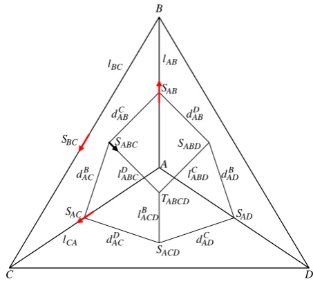
For sake of simplicity, at first, we assume in this paper that the circumcenter of a tetrahedron is located within the tetra-hedron. We consider a tetrahedronABCDwith the internal edgeAB (see Fig. 2) and the neighbouring elements, which share the edgeABwith it (see Fig. 3).

The electric field intensity components (marked with red color in Fig. 1 and in Fig. 2) are located at the centers of the edges of the tetrahedra, and the magnetic flux density com-ponents (marked with black color) are normal to the circum-centers of the triangular faces. The Voronoi cells are poly-topes. In the special case demonstrated in Fig. 1 the Voronoi cell is a pentadodecahedron which results as dual cell from 20 neighboring regular tetrahedra.

We use the following notations (see Figs. 1, 2, and 3) with X, Y, Z, W ∈ {A, B, C, D}, whereX, Y, Z, W are different from each other, in order to develop the grid equations for tetrahedral nets:

X, Y, Z, W nodes,

XY edge between the nodesXandY,

XY Z triangle,

XY ZW tetrahedron,

A

D

C

B

T

S

S

ABC ABD

Fig. 1. Voronoi cell and single tetrahedron.

SXY Z circumcenter of the triangleXY Z,

TXY ZW circumcenter of the tetrahedronXY ZW,

EXY magnitude of the electric field onSXY

between the nodesXandY,

BXY Z magnitude of the magnetic flux density

onSXY Z, normal toXY Z,

µXY ZW =µ0µr permeability inXY ZW,

XY ZW =0r permittivity inXY ZW,

lXY distance of nodeXto nodeY,

l_{XY Z}W distance of the circumcenter ofXY ZW to the faceXY Z,

d_XYZ distance of the circumcenter ofXY Z to the edgeXY,

aXY Z area of triangleXY Z.

EXY andBXY Zsatisfy

EXY = −EY X,

BXY Z= BY ZX= BZXY = −BY XZ = −BXZY = −BZY X ,

(10)

respectively.

Using a finite volume approach with the lowest-order in-tegration formulae (7) Eqs. (1) are transformed into a set of grid equations.

Taking into account the constitutive relations (2) the first equation of (1) is discretized on the dual grid. The internal edgeABis orthogonal to the corresponding Voronoi cell face over which we have to integrate (see Fig. 1). The closed integration path∂(see Eqs. 1 and 7) consists of the edges with lengthsi = lXY ZW (see Eq. 7 and Fig. 2), and is the

C D

A B

S S

S

S

S S

T S

d d

d d d

d

l

l l

l l

l

AC AD

AB

ACD ABC ABD

ABCD BC

ACD ADC ADB ABD ABC

ACB

ACDB

ABD C ABC

D

AB BC

CA

Fig. 2. Tetrahedron with partial areas of the Voronoi cell faces, which correspond to nodeA.

C D

A B

Fig. 3. Tetrahedra which share the edgeAB.

polygon around the periphery of the mentioned Voronoi cell face (see Fig. 1, upper pentagon). The vertices of the polygon are the circumcenters of the tetrahedra which share the edge AB with the tetrahedronABCD (see Fig. 3). fi = BXY Z

denotes the function values onSXY Z (see Fig. 2). is the

area of the Voronoi cell face.f =EABdenotes the function

value on the centerSAB. Thus, the discretized equation takes

the form: P

CDµABCD1

l_ABCD BABC+l_ABDC BABD=

 ωhP

CD

1

2ABCD d

C

ABlABCD +dABD lABDC

i EAB

(11)

where the sum is over those tetrahedraABCD, which share the edgeAB(see Fig. 3).

the mentioned triangle.fi =EXY denotes the function value

on the edgesXY. is the areaaABCof the triangleABC.

f = BABC denotes the function value on the circumcenter

SABCof the triangleABC. This yields the following form:

lABEAB+lBCEBC+lCAECA= − ωaABCBABC. (12)

Now we address the first of the surface integrals I

∪

([]E)·d=0, I

∪

([µ]H)·d=0, (13) reverting to the dual grid. In Eq. (13)∪is a closed sur-face with an interior volume. We have to integrate over the surface of the Voronoi cell. The surface of the Voronoi cell consists of all partial Voronoi areas, which belong to tetra-hedron edges, whose shared corner node isA(see Figs. 1, 2 and 3). A discretization formula, with similar form to the right-hand side of (11) is obtained, i.e.

X

B

" X

CD

1 2

d_ABC l_ABCD +d_ABD l_ABDC #

EAB

!

=0, (14)

with =ABCD, except for the additional outer summation

taken over all the nodesB neighboring A(in the primary grid).

For our final integral Eq. (13) the primary grid is used again, but now the integration is over the surface of the tetra-hedronABCD. As a consequence, the discretized form

−aABCBABC−aACDBACD+ +aABDBABD+aBCDBBCD =0

(15) can be deduced.

Equations (11) and (12) form a system of linear algebraic equations for the computation of the electromagnetic field. Substituting the components of the magnetic flux density the number of unknowns in this system can be reduced by a fac-tor of two:

P

CD

1

µABCD

l_ABCD aABC +

lC_ABD aABD

lABEAB +

+l D ABClBC

aABC EBC+

lD_ABClCA

aABC ECA+

+ l C ABDlBD

aABD EBD+

l_ABDC lDA

aABD EDA

=

=ω2

2 P

CDABCD d_ABC l_ABCD +d_ABD l_ABDC EAB.

(16)

Here, summation is taken over these tetrahedra ABCD, which possess the common edgeAB. Equation (16) has to be solved using the boundary conditions (5) and (6).

5 Eigenvalue problem

For the eigenvalue problem, we refer to the rectangular grids (Christ and Hartnagel, 1987).

The transverse electric mode fields (see Eq. 5) at the ports of a transmission line, which is discretized by means of tetra-hedral grids, are computed interpolating the results of the rectangular discretization.

The field distribution at the ports is computed assuming longitudinal homogeneity for the transmission line structure. Thus, any field can be expanded into a sum of so-called modal fields which vary exponentially in the longitudinal di-rection:

E(x, y, z±2h)=E(x, y, z)e∓ kz2h_{. (17)} kzis the propagation constant. 2his the length of an

elemen-tary cell inz-direction. We consider the field components in three consecutive elementary cells. The electric field compo-nents of the vectore(see Eq. 9)Exi,j,k+1,Exi,j,k−1,Eyi,j,k+1,

Eyi,j,k−1,Ezi,j,k−1,Ezi+1,j,k−1, andEzi,j+1,k−1 are expressed by

the values of cellkusing ansatz (17). The longitudinal elec-tric field componentsEzcan be eliminated by means of the

electric-field divergence equation (see first equation of (13)). Thus, we obtain an eigenvalue problem for the transverse electric fieldyon the transmission line region:

Gy=γy, γ =e− kz2h_+e+ kz2h_{−2= −4 sin}2_(hk

z).(18)

The sparse matrix G is in general nonsymmetric and com-plex. The order of G isn=2nxny−nb.nxnyis the number

of elementary cells at the port. The sizenb depends on the

number of cells with perfectly conducting material. The rela-tion between the propagarela-tion constantskz and the

eigenval-uesγ is nonlinear. The interesting modes of smallest attenu-ation are found solving a sequence of eigenvalue problems of modified matrices (see (Hebermehl et al., 2003b)) using the invert mode of the Arnoldi iteration (Lehoucq, 1995).

6 PML modes

We use the PML in order to calculate the eigen modes of open waveguide structures as well as for structures that re-quire electrically large computational cross sections. Using only magnetic or electric walls at the outer boundaries causes additional non-physical box modes. Those modes would affect the propagation behavior of the physical waveguide modes. Introducing the PML shifts these box modes within the eigenvalue spectrum, away from the physical ones. The difference, however, is not always large enough to be clearly detectable. Therefore, we need an additional criterion to dis-tinguish these PML modes from the desired physical ones. The PML modes are characterized by their high power con-centration in the PML area (Tischler and Heinrich, 2000). Thus, to eliminate the PML modes we calculate the magni-tude of the power flow of each computed mode in the PML (P(P )), in the waveguide region (P(W )), and in the total com-putational domain (P):

P =P(P )+P(W )=

R

(P )

(Et×H∗t,m)·d+

R

(W )

(Et×H∗t,m)·d.

A mode is specified as PML-mode if

r(P )= P (P )

P > ξ , (20)

with valuesξ =0.2, . . . ,0.6, found empirically.

7 Laser analysis

The presented method, although developed initially for mi-crowave structures (Hebermehl et al., 2001), is expanded to meet the special requirements of optoelectronic structure cal-culations. For optoelectronic devices frequencies of about several hundred THz are common. Thus the complex region containing the eigenvalues of potentially propagating modes grows substantially. A significantly higher number of eigen-value problems have to be solved within our algorithm. Ad-ditionally, the maximum cell size of the discretization should be less than ₁₀λ, whereλdenotes the wavelength in the mate-rial with the highest <([]). Additional mesh refinements have to be used for structure regions with highly varying fields. All this results in high-dimensional problems which have to be handled.

To reduce the execution times, in a first step the problem is solved using a coarse grid with lower accuracy require-ments in order to find the approximate locations of the inter-esting propagation constants. Anyway, the number of mod-ified eigenvalue problems to be solved is high. Thus, we split the interesting interval into subintervals and compute the corresponding eigenpairs independently and in parallel, for instance on different workstations or shared memory mul-tiprocessors. Finally, the modes of interest are calculated in a second step for an essentially reduced region using a fine grid, that fulfills higher accuracy requirements.

The linear sparse solver PARDISO (Schenk et al., 2000) is applied in order to fulfill the high accuracy requirements of the eigenvalue problem. The parallel CPU mode of PAR-DISO provides the additional possibility to reduce the com-puting times for this high-dimensional problem on shared memory multiprocessors without essential additional mem-ory requirements.

A Laser application can be found in (Hebermehl et al., 2003a).

8 Systems of linear algebraic equations

Four kinds of preconditioning and a block quasi-minimal residual algorithm are applied to solve the large scale sys-tems of linear algebraic equations. Details are given with (Schlundt et al., 2001) and (Hebermehl et al., 2003a).

Especially, adding the gradient of the electric field diver-gence the numerical properties of the system matrix are im-proved and the equations can be solved faster.

8.1 Rectangular grids

Multiplying (9) by D1s/2yields a symmetric form of linear

algebraic equations:

¯

Ax=0, A¯ =(Ds1/2ATDs/µ˜D−A1AD

1/2

s −k02DA˜) (21) withx=D1s/2e. The gradient of the electric field divergence []∇([]−2∇ · []E)=0 (22) is equivalent to the matrix equation

¯

Bx=0, B¯ =Ds−1/2DA˜B

T_D−1

V˜˜BDA˜D

−1/2

s . (23)

The rectangular matrix B is sparse and contains the values 0, 1, and−1 only. The diagonal matrix DV˜˜is a volume matrix for the 8 partial volumes of the dual elementary cell. Taking into account the boundary conditions (5) and (6) Eqs. (21) and (23) yields the formAˆx =bandBˆx =0, respectively, and

(Aˆ + ˆB)x=b, Aˆ + ˆB complex indefinite symmetric, (24) can be solved faster than Eq. (9).

In comparison to the simple lossy case the number of it-erations of Krylov subspace methods increases significantly in the presence of PML. Among others the speed of conver-gence depends on the relations of the edges in an elementary cell of the nonequidistant rectangular grid in this case. The best results can be obtained using nearly cubic cells. More-over, overlapping PML conditions at the corner regions of the computational domain lead to an increase of the magnitude of the corresponding off-diagonal elements in comparison to the diagonal of the coefficient matrix. This downgrades the properties of the matrix. Thus, overlapping PML should be avoided.

8.2 Tetrahedral grids

Equations (11), (12), (14) and (15) can be written in matrix form. Besides of the locations and values of the entries, the matrix representations of Eqs. (11) and (12) have the same structure as Eq. (8), and an appropriate (see Eq. 21) sym-metric form of linear algebraic equations can be deduced. Adding the gradient of the electric field divergence also gives a system which can be solved faster. Here, the gradient of the divergence at an internal point is obtained considering the partial volumes of the appropriate Voronoi cell. PML are not included.

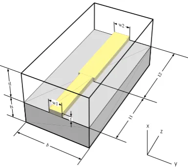
9 Application

As an example we have simulated a microwave structure with a microstrip changing its width (impedance step, see Fig. 4). The discontinuity of the metallic strip is located atz = l1. The metal is assumed to be ideally conducting. The relative permittivity of the substrate below the microstrip line isr = ˜

w1

w2

t ts

tl

b

l1 l2

x

y z

Fig. 4. The microstrip line changes its extension.

Measurements: b = 300µm, w1 = 60µm, w2 = 80µm, ts = 250µm, tl = 250µm, t = 3µm, l1 = 200µm, l2 = 200µm.

(r = ˜x = ˜y = ˜z =1). Ports are located at the planes

z = 0 andz = l1+l2. The remaining 4 outer surfaces are assumed to be electric walls. The structure is symmetric with respect to the planey =b/2. But, the whole structure is discretized in this test example.

For comparison the structure is subdivided in nonequidis-tant rectangular three-dimensional elementary cells on the one hand and in tetrahedra on the other hand.

In case of rectangular grids, the order of the system of lin-ear algebraic equations, which corresponds to the boundary value problem (1), isn = 3nxnynz = 335 160. nxnynz is

the number of cells of the structure which is assumed to be a parallelepiped. We need a high mesh refinement near the microstrip line. Using the rectangular grid the mesh refine-ment in this region results in an accumulation of elerefine-mentary cells in all coordinate directions even though the refinement is not necessary in order to approximate the solution with the required accuracy.

The tetrahedral grid consists ofnn =29 615 nodes,nt =

161 308 tetrahedra, andnp = 16 100 peripheral cell faces.

The order of the corresponding system of linear algebraic equations is equal to the number of edges and amounts n=nn+nt +np/2−1=198 972. (25)

The disadvantage of rectangular grids, the accumulation of elementary cells in all coordinate directions, is avoided here.

10 Conclusions

Finite-difference analysis of microwave circuits including lossy materials and radiation effects leads to an complex eigenvalue problem and large-scale complex indefinite sym-metric systems of linear algebraic equations. Staggered nonequidistant rectangular grids and tetrahedral nets with corresponding Voronoi cells are used. The high execution times in the eigenvalue problems for waveguide applications

with extremely large mesh sizes, e.g. laser structures, are re-duced using a coarse and a fine grid, and two levels of paral-lelization. The high-dimensional systems of linear algebraic equations are solved using a bock Krylov subspace method.

Acknowledgements. We thank F.-K. H¨ubner for his support in

preparing graphics.

References

Beilenhoff, K., Heinrich, W., and Hartnagel, H. L.: Improved Finite-Difference Formulation in Frequency Domain for Three-Dimensional Scattering Problems, IEEE Transactions on Mi-crowave Theory and Techniques, 40, No. 3, 540–546, 1992. Christ, A. and Hartnagel, H. L.: Three-Dimensional

Finite-Difference Method for the Analysis of Microwave-Device Em-bedding, IEEE Transactions on Microwave Theory and Tech-niques, 35, 688–696, 1987.

Hebermehl, G., Schlundt, R., Zscheile, H., and Heinrich, W.: Im-proved Numerical Methods for the Simulation of Microwave Cir-cuits, Surveys on Mathematics for Industry, 9, 117–129, 1999. Hebermehl, G., H¨ubner, F.-K., Schlundt, R., Tischler, T., Zscheile,

H., and Heinrich, W.: Numerical Simulation of Lossy Microwave Transmission Lines Including PML, Lecture Notes in Computa-tional Science and Engineering, Springer Verlag, 18, 267–275, 2001.

Hebermehl, G., H¨ubner, F.-K., Schlundt, R., Tischler, T., Zscheile, H., and Heinrich, W.: Simulation of Microwave and Semicon-ductor Laser Structures Including Absorbing Boundary Condi-tions, Lecture Notes in Computational Science and Engineering, Springer Verlag, 35, 131–159, 2003a.

Hebermehl, G., H¨ubner, F.-K., Schlundt, R., Tischler, T., Zscheile, H., and Heinrich, W.: Perfectly Matched Layers in Transmis-sion Lines, Numerical Mathematics and Advanced Applications, ENUMATH 2001, Springer Verlag Italia, pp. 281–290, 2003b. Lehoucq, R. B.: Analysis and Implementation of an Implicitly

Restarted Arnoldi Iteration, Technical Report 13, Rice Univer-sity, Department of Computational and Applied Mathematics, 1– 135, 1995.

Sacks, Z. S., Kingsland, D. M., Lee, R., and Lee, J.-F.: A Perfectly Matched Anisotropic Absorber for Use as an Absorbing Bound-ary Condition., IEEE Transactions on Antennas and Propagation, 43, 1460–1463, 1995.

Schenk, O., G¨artner, K., and Fichtner, W.: Efficient Sparse LU Fac-torization with Left-Right Looking Strategy on Shared Memory Multiprocessors, BIT, 40, 158–176, 2000.

Schlundt, R., Hebermehl, G., H¨ubner, F.-K., Heinrich, W., and Zscheile, H.: Iterative Solution of Systems of Linear Equations in Microwave Circuits Using a Block Quasi-Minimal Residual Algorithm, Lecture Notes in Computational Science and Engi-neering, Springer Verlag, 18, 325–333, 2001.

Tischler, T. and Heinrich, W.: The Perfectly Matched Layer as Lat-eral Boundary in Finite-Difference Transmission-Line Analysis, IEEE Transactions on Microwave Theory and Techniques, 48, 2249–2253, 2000.