Potential function based on secondary control of the microgrid

(1)

Potential function based on secondary control of the microgrid

A thesis report submitted to the School of Engineering and Energy, Murdoch

University, in partial fulfilment of the requirements for the degree of

Bachelor of Engineering

Student name: Hamad Alsharekh (30669245)

Supervisor: Dr. Gregory Crebbin

(2)

I

Acknowledgment

I would like to express my deep gratitude to my supervisor Dr. Gregory Crebbin for assisting me throughout my thesis course. Despite his busy schedule, Dr. Crebbin was always available to answer my questions and discuss my research findings with me. His valuable comments and advice gave me the confidence to overcome the challenges I faced throughout my thesis work.

I would also like to thank my lovely wife for her support and understanding during the times when I was too busy working on my thesis.

(3)

II

Abstract

(4)

III

1 Introduction

1.1

Definition of a Microgrid

A microgrid can be defined as a collection of small-scale electrical generators operating in parallel with the main grid to supply certain loads. It can also supply the load independently if there is a disturbance in the grid. Microgrid represents a new paradigm in electrical power distribution. It consists of multiple small generator sources, distribution storage, interconnection switches, and a control system. The small generator sources, which are also called microsources, can be either renewable sources or conventional generators. These sources are usually located near to the load. One of the greatest advantages of the microgrid is that it can operate in parallel with the main grid or it can work in islanded mode wherever there is a disturbance on the main grid.

1.2 Thesis Problem

(8)

2 1.3 Thesis Objective

Conflicts often exist between economists and environmentalists. Economists are usually concerned about money and financial costs, whereas environmentalists are more concerned about sustainability of the environment. A microgrid is a new paradigm that provides power with less impact on the environment. It uses relatively small renewable sources instead of upgrading the main grid with large generators. Therefore, the microgrid has been widely investigated. A large number of studies have been conducted on microgrid technology, such as its components, operation, and protection. The current paper investigates the following issues:

 Understanding microgrid concept and operations

 Hierarchical control strategies of the microgrid

 Understanding the potential function minimiser

 Using the potential function minimiser to remove the voltage deviation produced by the primary control by controlling the magnitude of the secondary voltage of the microgrid

(9)

3 1.4 Report Outline

Chapter 2 introduces the background to the microgrid, including its concept, need, component, and structure.

Chapter 3 focuses on microgrid operations and controls. The operation of a microgrid is conducted in both grid connected and islanded modes, as well as in the transitionbetween the two modes. The controls only focus on islanded mode operation.

Chapter 4 explains the potential function and how it can be used to control the magnitude of the secondary voltage.

Chapter 5 expounds on the selected system, explains how the system is connected, and presents the parameters of the system.

Chapter 6 shows the simulation platform and explains each simulation program used in the thesis as well as the reasons for using these programs.

Chapter7 presents the simulation results and discussions.

(10)

4

2.0 Background

2.1 Microgrid Concept

A microgrid is a network consisting of distributed generator and storage devices used to supply loads. A distributed generator (DG) in a microgrid is usually a renewable source, such as combined heat and power (CHP), photovoltaic (PV), wind turbine, or small-scale diesel generator. DGs are usually located near the loads, so that line losses in a microgrid are relatively low. A microgrid can work with a host grid connection or in islanded mode. when grid connected, DGs supports the main grid during peak demand. However, if there is a disturbance in the main grid, a microgrid can supply the load without the support of the main grid. Moreover, a microgrid can be reconnected when the fault in the main grid is removed [3]. Furthermore, as in any technology, microgrid technology faces many challenges. Many considerations should be taken into account, such as the control strategies based on of the voltage, current, frequency, power, and network protection.

2.2 Need for a Microgrid

(11)

5

some areas have harsh geographic features, making the main grid difficult to connect. Using a microgrid is the best solution to provide power to these areas. In summary, the most important issues that make the microgrid technology important are: [17]

 Load demand has increased worldwide.

 Microgrids use renewable sources, so they have less impact on the environment.

 Extending the main grid is not only costly but also difficult.

 A microgrid can supply critical loads even if it is disconnected from the main grid.

2.3 Microgrid Structure and Components

Figure 1 shows the structure of a microgrid. The main grid is connected to the microgrid at the point of a common coupling. Each microgrid has a different structure (number of the DGs and types of DGs), depending on the load demand. A microgrid is designed to be able to supply its critical load. Therefore, DGs should insure to be enough to supply the load as if the main grid is disconnected. The microgrid consists of microsources, power electronic converters, distributied storage devices, local loads, and the point of common coupling (PCC). The grid voltage is reduced by using either a transformer or an electronic converter to a medium voltage that is similar to the voltage produced from the DG [2]. The components of the microgrid are as follows.

(12)

6 2.3.1 Microsource

A microsource is a small-scale energy source located near a load. It can be either a dispatchable or a non-dispatchable energy source in a microgrid network. The difference between the dispatchable and non- dispatchable unit is that the dispatchable unit is considered a voltage source because the amount of voltage output can be controlled. In contrast, the non- dispatchable unit is considered a current source, in which the output voltage level cannot be controlled. An example of a non- dispatchable unit is the PV panel. PV ceases to produce energy if there is no sun. However, in a voltage source, the voltage amount can be controlled (i.e., turned on/off) or increased/decreased depending on the voltage required for the microgrid load. The voltage from generators can be controlled by controlling the speed of the generators.

Microsources are usually small scale, less than 50 MW. They can be present as renewable source in the device in the form of CHP, solar PV, wind turbine, or fuel cell [3]. Furthermore, the voltage of microsources can be DC or AC, depending on the type of the microsource. For example, PV produces DC voltage, whereas wind produces AC voltage. Therefore, microsources are usually connected to a power electronics converter. One of the advantages of microsources is that line losses are reduced as microsources can be located near the load. In sum, a microsource is part of a microgrid. It can be a dispatchable or a non-dispatchable unit that can a produce DC or AC voltage. It is usually connected to inverters and is located close to the load [17].

2.3.2 Power Electronics Converters

(13)

7

For example, if the DG is a PV panel, the voltage produced is in DC form. Therefore, the voltage should be converted from DC to AC to match the voltage type of the microgrid load. Another example is that the voltage produced by wind turbine is AC, but it is not in the desired magnitude and phase. Thus, the voltage should be converted from AC to DC and from DC to AC with acceptable magnitude and phase.

The terms inverter and converter should not be used interchangeably. The inverter changes the DC voltage to AC voltage, whereas the converter changes the magnitude of the AC voltage. Converters can step up or step down the voltage produced by DGs. The power electronics converter also serves as a control device that can be used to control the voltage and frequency of DGs. Therefore, the amount of the voltage and frequency can be produced at a certain value by adjusting the converter.

2.3.3 Microgrid Load

The load of the microgrid can be houses, hospitals, banks and malls. This loads can be classified into two types. The first type is called critical load, examples of which are a hospital or a bank’s computer system. As indicated by the examples, critical load should be supplied with an uninterruptible energy source that has high power quality. The second type is called uncritical load, examples of which are park lights or air conditioners or streetlights. Uncritical loads can be disconnected when there is a shortage of power supply or if the main grid is disconnected [2]. Uncritical loads are usually supplied by a current source, such as PV, or storage devices.

(14)

8 2.3.4 Storage Devices

(15)

9

2.3.5 Control System

The control system is an important component of the microgrid operation because it ensures that the system works correctly. For example, if it is working optimally, the carbon emission will be reduced as generators will run with less fossil fuels. Moreover, the transfer from one mode to other is conducted safely. A microgrid commonly requires a microsource controller (MC) and a central controller (CC). Each type of control system is discussed in the following subsections [16].

2.3.5.1 Microsource Controller MC

Using the MC is considered the first step in microgrid control. The MC has the benefit of using the power electronics devices built into the DG sources. It uses local information about the microgrid status and functions depending on the microgrid status. The MC controls the voltage and frequency of the microgrid [14]. This control enables the DGs to maintain their power output if the load changes or switches to the islanded mode or reconnect to the main grid. Therefore, DGs respond according to the system changes. One of the advantages of the MC is that it responds quickly to any disturbance or load change. Moreover, using this type of controller does not require communication between the DGs. The MC control strategy uses the P-F and Q-V control methods, which are the droop control methods. The MC usually acts as the primary control, which will be discussed in detail later [3].

2.3.5.2 Central Controller CC

(16)

10

the entire MC. The new set points of the voltage and frequency are sent from the CC to the MCs to ensure that the operation of the microgrid is performed optimally. Moreover, the CC is used to update the set points of the voltage and frequency when the host grid is disconnected from the microgrid. It updates the new set points when the main grid is reconnected to the microgrid after the disturbance is removed. The CC acts as a secondary controller respond more slowly than the MCs.

According to [13], the key functions of the CC are

 to provide the individual power and voltage set points for each DG controller,

 to minimize emissions and system losses,

 to maximize the operational efficiency of the microsources, and

 to provide logic and control for islanding and reconnecting the MG during events.

2.3.6 Point of Common Coupling PCC

(17)

11

3.0 Microgrid Operation

This chapter briefly introduces the microgrid operation. The microgrid operation modes, i.e., grid connected, islanded mode, and transition between the grid connected and islanded modes, are discussed. The important issues considered for each operation mode are introduced as well. However, only the islanded mode is discussed in detail, as the current paper focuses on the behaviour of the microgrid in islanded mode.

3.1 Grid Connection

The grid connection mode is the normal operation status of the microgrid. In this mode, the load is supplied by both the grid and the microgrid. The voltage of the grid is determined by the PCC. The voltage of the grid should be in the same phase as the voltage generated by the DG. Therefore, in the grid connection mode, the voltage and frequency of the DG are controlled by the grid voltage and frequency. More information about the grid connection mode can be found in [14, 17].

3.2 Islanded Mode

(18)

12

3.3 Transition between Grid Connection and Islanded Mode

The third type of operation mode of a microgrid is the transition between grid connection and islanded mode. The transition operation of a microgrid is the time between the microgrid disconnection from the grid and the reconnection to the grid. In this situation, the voltage amplitude and frequency should be controlled to be within the acceptable limits to ensure the safe transition from one mode to another. At this stage, the static switch adjusts the power reference to the desired value. The voltage and frequency can be measured inside the microgrid. The maximum value allowed for the change in voltage and frequency is 2% for frequency and 5% of the voltage amplitude. More information can be found in [14, 17].

3.4 Hierarchy of Microgrid Controls

Microgrids have three levels of control: primary control, secondary control, and tertiary control. Microgrids should operate with these controls to ensure stable operation. This section expounds on the primary and secondary controls for islanded mode only. A thorough explanation on the tertiary control level can be found in [17]

Figure2: Hierarchy of Microgrid Controls [17]

(19)

13

Primary control is considered the first level of the microgrid control. This control strategy is implemented in each DG. This strategy is conducted using the P/Q control method. In the P/Q control strategy, real power is controlled by the frequency, and reactive power is controlled by the voltage. This strategy is expressed in the following equations:

The droop method is used for primary control and for controlling the microsources themselves. Moreover, as previously mentioned, this type of control does not require inter-source communication. The main aim of primary control is to control the voltage and frequency of the microsources. It ensures that each DG generates within the acceptable limit of the voltage and frequency by controlling the real and reactive power of the microsources.

Figure 3: Droop Control [14]

(20)

14

where ω and E are the amplitude frequency and voltage output, respectively, and ω*, E*, P*, and Q* are the frequency, voltage, real power, and reactive power references, respectively. m and n are the slopes of the equations. The reference of the real and reactive power is usually set to zero. The voltage magnitude and frequency delivered by DGs can be adjusted using these equations. [14]

3.4.2 Secondary Control

(21)

15

4.0 Potential Function Minimiser

In this chapter, an explanation about the potential function minimiser will be introduced. The potential function minimiser, its definition, advantages, components, and way of using it as a secondary voltage control of the microgrid will be mentioned in this chapter.

In this thesis, the potential function is used as a secondary control of the voltage of the microgrid in islanded mode. This function is based on the solution to a rendezvous problem. In a rendezvous problem, one point tries to reach the other point within a time limit, as explained in [1]. Therefore, this method determines the common set point that converges on that set point. Different methods can be used to implement the rendezvous problem [10]. One such method is the potential function. The reason for selecting the potential function for secondary voltage control is straightforward, as adding more terms to the expression is more flexible. Moreover, the potential function can be used to solve any problem involving a vector variable by replacing the vector variable with a scalar variable [2].

In the next section, more information about the potential function will be presented.

4.1 Definition of Potential Function

A potential function is a positive scalar function. It is used to reduce three vector functions into a scalar function with one component [18]. Potential functions have been used in many areas, such as in electronics, mechanics, control of robots, and control of microgrids [11]. In the case of the microgrid, the potential function is defined in each DG to remove the deviation produced by the primary control.

………(1)

(22)

16

Where a potential function and Xj is is the vector value of the set point of the secondary control of the microgrid. Xj can be the vector set point value of real power P, reactive power Q, voltage, or current in the microgrid. Moreover, when the deviation is eliminated, the new set point should be found in the system. The new set point with the desired value can be determined using the gradient descent method, as shown in the following equation [10]:

... (2)

where is the new set point

is the old set point

K is the constant that adjusts the magnitude of the change in set point

is the time between the new and old set points

The differential part gives the minimum value of the potential function.

The potential function minimiser used in the microgrid has the following advantages [11]:

1) Potential functions can be easily implemented in the system.

2) More terms can be added in the function if one or more voltage terms are added. 3) It can be used to control the frequency as well.

4) Potential functions enable the voltage to be controlled from the operation point until the desired magnitude of the voltage is obtained.

(23)

17

4.2 Potential Function Based on the Microgrid Control

The potential function minimiser reduces the difference between the measurement value and the goal value. This method appoints the goal value as the set point and compares the measurement value, which is the voltage generated by DGs. The bus voltages are measured and compared with the goal values. If the generated values are not in the desired magnitudes, the CC corrects the voltage magnitude generated to be the same as the goal value [9]. This correction can be done when the microgrid is in the desired state. The desired state of a microgrid can be reached when all DGs have reached their steady state without set point error. In other words, the secondary control begins after the primary control is conducted to avoid the decoupling between the primary and secondary controls. For the secondary control, the desired state refers to the minimum value of the potential function, which may or may not reach zero depending on the equation of the potential function. Moreover, to perform the secondary control, communication between the CC and each DG is required because the CC calculates the new point according to Equation (2) and sends the new set point to each DG. Therefore, two-way communication is required for the secondary control to enable the CC to receive and send information to and from the DG. Communication between the CC and the DG can cause some delay, but the delay will not affect the system as the secondary control controls the microgrid [10].

4.3 Components of the Potential Function

The components of a potential function consist of three terms. The first term corresponds to the measurement of each DG. The second term is a constraint term that deals with the limitation of the voltage value, which should not exceed a certain value for each DG [10]. The last term is the goal value (set point) of the DG, which is called the desired value. The potential functions can be written as [10]:

(24)

18

where & are the weight factors of the measurement, constraint, and goal, respectively, and & are the partial potential functions of the measurement, constraint, and goal for each DG. A weight factor is also used depending on the importance of the measurement term. For example, if the value of the goal is more important than that of the measurement, the goal term should be multiplied by the weight factor.

The parameters should be defined for each DG. These parameters are used in conjunction with Equation (1) for each updated set point. Therefore, each term of the potential function equation has a partial derivative according to Equation (2). Each derivative of each term has the following benefits [10]:

1) Partial derivative of the measurement provides a flat voltage as well as controls the power flow of the microgrid.

2) Constraint partial derivative makes the system stable with an acceptable operation level of the DG.

(25)

19

5.0 Test Microgrid System

The system and method selected as the model for this thesis were obtained from [10]. The model is a part of the North American medium voltage system. The microgrid consists of two DGs that feed the two critical loads, and it can work in the grid and islanded modes. Three assumptions are made for the operation of the selected system. First, the system is controlled by the primary control; second, the frequency is fixed and reaches a steady state; and third, the load demand can be met by its own DGs. Figure 4 presents the microgrid system.

Figure 4: Two-DG Cascade Microgrid System [10]

The main grid is strong with an SCMVA of 12000 MVA and X/R ratio of 0.1. The main grid is

(26)

20

impedance connected in parallel with a capacitor. The power factor for each load is adjusted to 0.95. Each load has its own load limit. Load 1 has a limitation of 240 kVA, and the second has a limitation of 435 kVA. Both loads are assumed critical loads that should be supplied all the time.

Furthermore, the microgrid is supplied by two small DGs. In this system, the two DGs are considered the voltage sources. The voltage produced by the DGs is 480 V L-L. Each DG is connected to a transformer. The voltage from the DG is stepped up by the transformer from 480 V to 12.47 kV. The system contains three buses, with each bus connected to a load. At PC1, the bus corresponds to load 1, and at PC2, the bus corresponds to load 2. The remaining bus is PCC, which is connected to the grid generator. A filter impedance is connected to each DG. The Impedance between PC1 and PC2, represents an overhead line. The parameters of the system are presented in Table 1.

Parameter Value Value pu

Fundamental frequency f=60 HZ

Switching frequency 1620 HZ 27 pu

Grid voltage Vs=230 kV

Grid resistance RS=0.439 Ω

Grid inductance LS=11.635 mH

Transformer G 230 kV/12.47 kV 0.013+j1.55 Ω 0.001+j0.120 pu

Transformer 1 12.47 kV/480 V 500 KVA 0.005+J0.080 pu

Transformer 2 12.47 kV/480 V 300 KVA 0.005+J0.080 pu

DC bus voltage Vdc= 1200 V

Filter impedance 0.025+j0.040 pu

Line 1 0.846+j2.112 Ω (Ll1=5.603 mH)

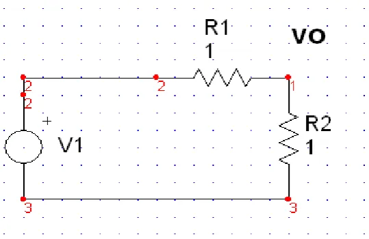
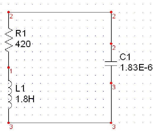
Load 1 240 KVA R=810 Ω, L= 2.86 H, C=1.38 µF

Load 2 435 KVA R=420 Ω, L= 1.80 H, C=1.83 µF

Table1: Parameters of the Tested System [10]

(27)

21

two buses. In islanded mode, the microgrid is initially controlled by the primary control. This control produces a voltage deviation that affects the magnitude of the voltage, making it less than the desired voltage magnitude. The CC checks this deviation. The CC updates the DG to provide a voltage at each bus of 1 pu. After the updating from the CC, the DG generates a voltage of 1 pu at each bus. The voltage produced by the DGs should be more than 1 pu, considering that the voltage droops in each voltage source are caused by the filter and transformer impedances.

In the current thesis, calculation of the new voltages is conducted with care. As the voltage at each bus must be 1 pu, the voltage of the DG is calculated as a function of the voltage at the PCs. This calculation is conducted using the Thevenin voltage [5]. Using the Thevenin theorem, the circuit not only becomes a simple series circuit, but the voltage detected by the load can also be found. The procedure for calculating the system as well as the actual calculation can be found in Appendix D. After the calculation, as well as determining the value of each DG, the potential function minimiser reduces the voltage at both PCs. The system is implemented in single phase as it is assumed the system is balanced.

function y=M(x)

M=@(x)((0.622)*x(1)+(0.367)*x(2)-1)^2+((0.611*x(2)+(0.3768)*x(1)-(0.622)*x(1)-(0.367)*x(2)))^2; [x] = fminsearch(M ,[0, 0])

V1=(0.611)*x(2)+(0.3768)*x(1) V2=(0.622)*x(1)+(0.367)*x(2) M=(V1-1)^2+(V1-V2)^2

end

The values of VDG1, VDG2, V1, and V2 from Matlab are as follows: x = 1.0093 1.0142

algorithm: 'Nelder-Mead simplex direct search' V1 =1.0000 V2 = 1.0000

(28)

22

6.0 Simulation Platform

6.1 Matlab

(29)

23 6.2 Simulink and Powerlib

Matlab Simulink is a simulation program that enables users to build and test an electrical network. This simulation is considered as a simple simulation, as electrical parameters are already built into the program. An electrical circuit can be built in Simulink using the parameters in the Powerlib library, where most of the circuit components already built as boxes can be found. More information about how Matlab Simulink and Powerlib can be used is available in [6, 15]. Simulink also shows the waveforms of the output. It contains a box called simout, where the actual data of the output can be found. Therefore, the voltage at each bus can be verified as a waveform and data.

(30)

24

7.0 Simulation Results and Discussions

The potential function minimiser is written as code in Matlab. Afterwards, the result is checked in Powerlib in Simulink. One phase is implemented in Simulink, as the system is assumed to be balanced. The desired magnitude of the voltage at each bus is assumed to be 1 pu, after the voltage is to be generated by the DG, is found in Matlab. The voltage of the DGs is a function of the voltage at each bus. This method is performed in Matlab to determine the value of the voltage produced by each DG and to minimise the voltage difference between each DG with the voltage at each bus. The components of the network, such as voltage sources and impedances, can be found in the Powerlib library, and so Powelib is used.

This section presents and discusses the results of the simulation. Starting the control experiment with a simple circuit is always recommended because it provides a thorough and deeper understanding of the main idea. As a starting point, only the simple circuit in figure 5 is selected, which contains a voltage source and two resistances, a resistive line and a resistive load. The task of this system is to determine the input voltage as a function of the output voltage. The voltage output must be 5 V. The system and the calculation seem easy, but they should be understood as just a first stage because they have similar concept to the main system. The two voltage values should be maintained to provide the desired magnitude of voltage at the load. The voltage at each bus should be minimised as well. Therefore, in the simple example, the potential function is used to adjust the voltage input in order to make the voltage output equal to the desired value. Potential function to be minimised for this system is:

(31)

25

For the system in figure 5, the potential function tries to minimise the voltage difference between the output and the desired voltage magnitude. Therefore, the voltage input should be 10 V to satisfy the conditions of the voltage being equal to 5 and the potential function minimiser converging to be equal to zero. Moreover, assume the desired voltage magnitude is changed from 5v to 10v, so the voltage input will produce an input voltage of 20v to minimize the potential function. This method ensured that whenever the voltage set point is changed the voltage input will be changed to minimize the potential function.

Figure 5: Implementation of the Simple System

(32)

26

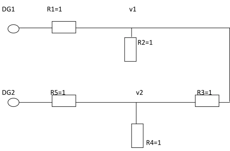
difficult one. Therefore, the system is upgraded to the all- resistive network shown in figure (6), the value of each resistance is 1 Ω.

The system transfer function is calculated using the Thevenin method (see Appendix A). The Matlab minimising function is used to determine the voltage value for each DG in order to minimize the voltage magnitude at each bus.

DG1 R1=1 v1

R2=1

DG2 R5=1 v2 R3=1

R4=1

Figure 6: System Equivalent Circuit with Resistance

(33)

27

The potential function minimiser equation of this system is

The first term of the equation attempts to make the voltage at bus 2 equal to 1, as the desired magnitude at that bus is 1 pu. The second term makes the magnitudes of the voltages at bus 1 and bus 2 close to each other. As the magnitude of voltage at each bus should be a positive magnitude, the two parts of the equation should be squared to ensure a positive magnitude. This potential equation should be defined for each DG. Before, the calculation is carried out in Matlab, a hand calculation is performed to determine the values of VDG1 and VDG2. The hand calculation gives a value of VDG1=2 and VDG2=2. Therefore, based on the hand calculation, the values of VDG1 and VDG2 should be 2 if the potential function is equal to zero. Implementing the equation in Matlab yields the following:

function y=G(x)

G=@(x) (0.375*x (2) +0.125*x (1)-1) ^2+ (0.25*x (1)-0.25*x (2)) ^2; [x] = fminsearch(y, [0, 0])

v2= (3*x (2) +x (1))/8 V1= ((3*v2)-(x (2))) G = (v2-1) ^2 + (V1-V2) ^2

end

The solution obtained from Matlab is as follows: x =

(34)

28

The function is passed in the minimisation function to find the minimum value of the VDG1 1 and VDG2 2. This minimum value makes the voltage at bus 1 and bus 2 at close or equal to the desired magnitude. Also, if the desired magnitude is change to different value, the magnitude VDG1, VDG2 will be change to make the potential function is equal to zero. More information about the minimisation function in Matlab fminsearch can be found in [4].

The Matlab result confirms the accuracy of the result of the hand calculation. Therefore, the fminserach function in Matlab is a suitable minimiser function.

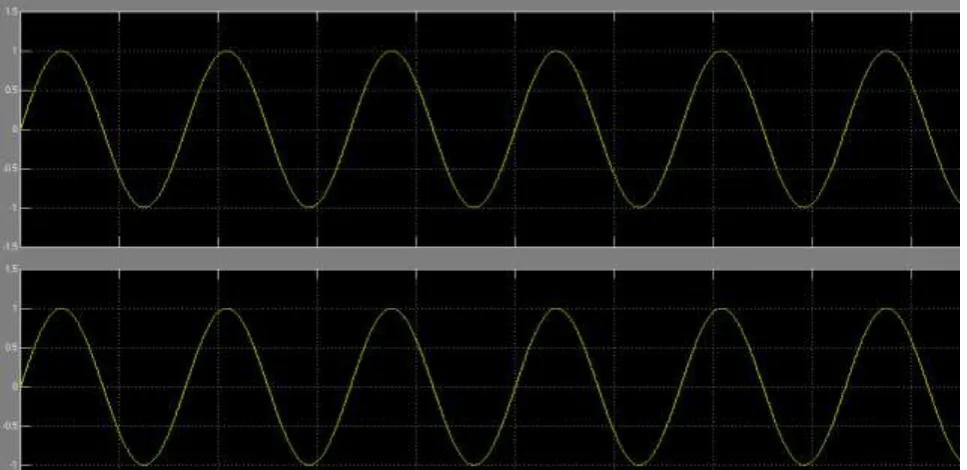
The system is also implemented in the Powerlib library in Simulink to verify that the magnitude of the voltage is the correct value, as well as checking that the method is correct. In the Powerlib simulation, the magnitude of the voltage for the DGs is specified by the user as equal to 2 V. The voltage at each bus, which corresponds to the load, is measured to check if it will be equal to 1 V. In the Powerlib implementation, which is the opposite of the Matlab method, the voltage of DG is equal to 2 V. The voltage at bus 1 and bus 2 is measured. Figure 7 shows the voltage magnitude at each bus. The implementation of the system can be found in Appendix C.

(35)

29

As shown in the figure, the voltage magnitude at each bus is equal to 1 V. Therefore, this result proves that the hand calculation and the Matlab calculation are both correct. In the next section, the actual system is tested in Matlab.

Actual system

After calculating and using the minimising function in the simple system, the actual system is implemented in the same way. In this system, all values are converted into per unit value to avoid the transformer impedance calculation at the high and low sides. The voltage magnitude at bus 1 and bus 2 is assumed 1 pu. This value is only the magnitude of the voltage. Therefore, after calculating the voltage at bus 1 and the voltage at bus 2 as a function of the voltage produced by the DGs, the values of V1 and V2 are represented as complex numbers. These complex numbers should be converted into polar form, as only the voltage magnitude is needed, as only the magnitude of the voltage will be minimised and not the angle. The same steps as in the previous example are followed. The magnitude of the voltage produced by the DGs can be calculated to provide the desired value for bus 1 and bus 2. The calculation is conducted in Matlab using the fminsearch function when the voltage is set to be equal to 1 pu at each bus. Many values can be chosen, but only the minimising function used as the minimum value is shown in Matlab. Thus, the voltage magnitude produced from DG1 is 1.009 pu, and the voltage from DG2 is 1.0142 pu. The voltage produced by DG1 and DG2 makes the voltage at each bus at desired voltage magnitude as well as the voltage magnitude at each bus is close to each other. However, if the desired voltage magnitude is changed the VDG1 and VDG2 will be change to make the voltage at each bus close to the desired magnitude. Therefore, whenever the desired voltage magnitude is change the potential function ensures that the voltage generator will be changed.

(36)

30

should be recalculated from the per unit value to the normal value because the Powerlib program does not accept per unit values. The voltage and impedance values can be calculated by multiplying the per unit value by the voltage base, which is 480v, and the impedance base 311 Ω respectively. Therefore, the voltage generated by DG1 is equal to 484.47 V, and the voltage produced by the DG2 is 486.58 V. Afterwards, the voltage at bus 1 and bus 2 is measured. The implementation of the system can be found in the appendix C. Figure 8 shows the result obtained from Powerlib.

Figure 8: Voltage Output of V1 and V2 for Actual System

(37)

31

8.0 Conclusions and Future Works

8.1 Conclusions

(38)

32 8.2 Future Works

In extending this thesis, many areas can be exploited and developed with the chosen system:

1) The primary control of this system can be implemented.

2) The frequency deviation produced by the primary control can be controlled, as the frequency in the current thesis is assumed fixed.

3) The tertiary control of the system can be implemented. 4) The full dynamic modeling of the DG can be investigated.

(39)

33

9.0 References

[1] Alpern, Steve. (1995). The rendezvous search problem. SIAM Journal on Control and Optimization, 33(3), 11.

[2] Basak, Prasenjit, Saha, A. K., Chowdhury, S., & Chowdhury, S. P. (2009). Microgrid: Control techniques and modeling. Paper presented at the Universities Power

Engineering Conference (UPEC), 2009 Proceedings of the 44th International Glasgow.

[3] Chowdhury, Sunetra, Crossley, Peter & Chowdhury, S. P. (2009). Microgrids and active distribution networks. London: Institution of Engineering and Technology.

[4] Clark, Andy. (2011). Fminsearch Retrieved from

http://www.mathworks.com/help/techdoc/ref/fminsearch.html

[5] Hambley, Allan R. (2011). Electrical engineering : Principles and applications (4th ed). Upper Saddle River: Pearson Education

[6] Karris, Steven T. (2006). Introduction to simulink with engineering applications. Fremont: Orchard Publications

[7] Ketjoy, Nipon, Chimtavee, Amnaj, Mensin, Yodthong, Mansiri, Kongrit & Srikeaw, Suchat. (2011). 120 kw pv microgrid system. Retrieved 9 October, 2011, from

http://www.sert.nu.ac.th/re_mg.htm

[8] Kueck, J. D., Staunton, R.H., Labinov, S. D. & Kirby, B.J. (2003). Microgrid energy management system (U.S. DEPARTMENT OF ENERGY, Trans.). Tennessee: The Consortium for Electric Reliability Technology Solutions (CERTS)

[9] Mehrizi-Sani, Ali, & Iravani, Reza. (2009). Secondary control for microgrids using potential functions: Modeling issues. Paper presented at the Conference on Power Systems, Canada.

[10] Mehrizi-Sani, Ali & Iravani, Reza. (2010). Potential-function based control of a microgrid in islanded and grid-connected modes. IEEE Transactions on Power Systems, 25(4), 8.

[11] Mehrizi-Sani, Ali & Iravani, Reza. (2011). On the educational aspects of potential

(40)

34

[12] Nikkhajoei, Hassan & Lasseter, Robert. (2009). Distributed generation interface to the certs microgrid. IEEE Transactions on Power Delivery, 24(3), 10.

[13] Pilo, F., Pisano, G. & Soma., G.G. (2007). Neural implementation of microgrid central controllers. Paper presented at the Industrial Informatics, 2007 5th IEEE International Conference Vienna.

[14] Quintero, Juan Carlos Vasquez. (2009). Decentralized control techniques applied to electric power distributed generation in microgrids. PhD, Universitat Politècnica de Catalunya.

[15] Stanoyevitch, Alexander. (2005). Introduction to matlab with numerical preliminaries Hoboken: Wiley-Interscience

[16] Tsikalakis, Antonis & Hatziargyriou, Nikos. (2008). Centralized control for optimizing microgrids operation. IEEE Transactions on Energy Conversion, 23(1), 8.

[17] Vasquez, Juan, Guerrero, Josep, Miret, Jaume, Castilla, Miguel & Vicuna, Luis Garcia de. (2010). Hierarchical control of intelligent microgrids. IEEE Industrial Electronics Magazine 4(4), 7.

[18] Weisstein, Eric W. (2011). Potential function. Retrieved 8 October, 2011, from

(41)

35

10.0 Appendices

10.1 Appendix A

Appendix A presents the system calculation, including impedance calculation, per unit calculation, and the calculation of the voltage generated by each DG.

Figure A.1: Microgrid Selected System

Load 1: RLC circuit

The calculation of the impedances of each load is as follows: For the first load

(42)

36

(43)

37 Load2: RLC circuit

For load 2, the following parameters are given: R1=420 Ω, L= 1.80 H, and C=1.83 µF.

Figure A.3: Impedances of Load 2

(44)

38 Voltage equations of the DGs:

The voltage of DG1 and DG2 is calculated. The equivalent circuit is shown as follows.

DG1 .025+j0.04 0.005+j0.08

7.03+j1.145

DG2 025+j0.04 0.005+j0.08 0.003+j0.008

3.86+j2.1

Figure A.4: Equivalent Circuit of the Selected System

DG1 z1=0.03+j.12

v1

Z2=7.03+j1.145

DG2 Z5= 0.03+j.12 v2 Z3= 0.003+j0.008

Z4= 3.86+j2.1

(45)

39

The voltage V1 and V2 should be 1 pu. Therefore, the voltage generated in DG1 and DG2 should be calculated and minimised to produce V1 and V2 1 pu. The voltage in DG1 and DG2 is calculated. The equivalent impedances with respect to V2 should be calculated.

DG1 z1=0.03+j.12 Z3= 0.003+j0.008 Z5= 0.03+j.12

Z2=7.03+j1.145 Z4= 3.86+j2.1

DG2

Figure A.6: Equivalent Impedances with respect to V2

Zeq=[(Z5//Z4)+(Z3)//Z2]+Z1

Z3= 0.003+j0.008 Z5= 0.03+j.12

Z2=7.03+j1.145 Z4= 3.86+j2.1

I1 I2 I DG2

(46)

40

Z5= 0.03+j.12

Z2=7.033+j1.153 Z4= 3.86+j2.1

I1 I2 I DG2

Figure A.8: Equivalent Circuit for the Selected System after Adding Z2+Z3

2.5+J1.145 VDG2 I

Figure A.9: Equivalent Circuit of A.8

(47)

41 The same procedure is performed for V2, which yields

DG1 z1=0.03+j.12

v1

Z2= 3.86+j2.1

DG2 Z5= 0.03+j.12 v2 Z3= 0.003+j0.008

Z4=7.03+j1.145

(48)

42 Zeq=[(Z5//Z4)+(Z3)//Z2]+Z1

Zeq=0.07+j0.311 pu

Z3= 0.003+j0.008 Z5= 0.03+j.12

Z2=3.86+j2.1 Z4=7.03+j1.145

I1 I2 I DG2

Figure A.11: Equivalent Circuit for the Selected System after Removing Z1

Z5= 0.03+j.12

Z2=3.68+j2.108 Z4= 7.03+j1.145

I1 I2 I DG2

Figure A.12: Equivalent Circuit for the Selected System after Adding Z2+Z3

2.53+J1.145 VDG2 I

(49)

43

Substitute 3 into 1

From Equation 4, the equation of I1 is

Finding I2 can be done by substitute Equation (5) into (3) yielding

(50)

44 10.2 Appendix B

Matlab

After determining the equations for voltage at load 1 and load 2, the equations are implemented in Matlab to obtain the value of the voltage produced by DG1 and DG2 and to find the minimum value of the voltage for the desired voltage at buses 1 and 2. The voltage of DG1 and DG2 can be determined using Matlab; the value of the buses should be 1 pu.

The Matlab function called fminsearch, which finds the minimum value of a function, is used. More details about the fminsearch can be found in the Matlab help section. The potential function used for the system is

P=(V1-d)^2+(v1-v2)^2 Where

V1 is the voltage at load 1.

V2 is the voltage at the load 2.

d is the ‘desired voltage magnitude’ in bus 1.

(51)

45

function y=M(x)

M=@(x)((0.622)*x(1)+(0.367)*x(2)-1)^2+((0.611*x(2)+(0.3768)*x(1)-(0.622)*x(1)-(0.367)*x(2)))^2; [x] = fminsearch(M ,[0, 0])

v1=(0.611)*x(2)+(0.3768)*x(1) v2=(0.622)*x(1)+(0.367)*x(2) M=(v1-1)^2+(v1-v2)^2

end

The values for the VDG1, VDG2, V1, and V2 from Matlab are shown as follows: x = 1.0093 1.0142

algorithm: 'Nelder-Mead simplex direct search'

(52)

46 10.3 Appendix C

Validating the Matlab Results in the Powerlib Simulation Program

The solutions determined using Matlab should be verified to determine their accuracy. A single system is built in the Powerlib Simulink. The system consists of two voltage sources connected to the RL impedance, which is equivalent to the filter and transformer impedances. Each source also provides a voltage to the bus PC1 for load 1 and PC2 for load 2. The voltage sources supply 1.0093 pu for DG1 and 1.0142 pu for DG2. The voltage base is 480 V. Therefore, the voltage for DG1 is 484.5 V, and the voltage for the DG2 is 486 V. Afterwards, the voltage at PC1 and PC2 is measured to ensure that the voltage is 1 pu. The value of the voltage can be determined by connecting the simout at PC1 and PC2. The diagram below shows how the system is connected.

For a simple system with resistance only,

(53)

47

Figure C.2: Block Parameter for DG1

(54)

48 For the actual system

Figure C.4: Implementation of the System in Powerlib

(55)

49

Figure C.6: Block Parameter for DG2

(56)

50

Figure C.8: Simout Data for V2

(57)

51 9.4 Appendix D

Thevenin calculation

For system selected in Figure [1], the thevenin voltage is calculated. In this section, how the voltage of the DG is calculated is introduced in detail for the information of the readers.

1) The base impedance should be calculated by Zbase= (vbase) ^2/sbase.

2) All the impedances are converted in the per unit value using Zpu=Z/Zbase, which is shown in the following diagram.

DG1 z1 v1

Z2

DG2 Z5 v2 Z3

Z4

(58)

52

3) Calculate the equivalent impedance of the system by Zeq= [(z5//z4+z3)//z2+z1]

DG1 z1 Z3 Z5

Z2 Z4

DG2

Figure D.2: Thevenin Circuit as Observed by Load 1 with the Equivalent Circuit for the Selected System

4) Remove Z1 because there is no current following this impedance that yields the circuit below:

Z3= Z5=

Z2 Z4

I1 I2 I DG2

(59)

53

5) Find the new equivalent impedance after removing the first impedance.

6) Find the equation for the current sI1, I2, and I. that can be performed by the following equation:

I=I1+I2………....1 (z2+z3)I1=z4*I2….2 I1=(z4/(z2+z3))…….3

Substitute Equation 3 into 1 to determine the equation of I1 and I2 in terms of I 7) Find Veq, which the voltage as observed in z2:

Veq=I1*z2

8) The current equivalent should be found by Ieq= VG2-(Veq*vg1)/zeq

9) V1, which is at bus PC1, can be calculated by V1= - (Ieq*Z1) +VG2

For the voltage across load 2 of v2, the same steps should be followed, but the impedance should be rearranged opposite of the arrangement of the voltage for load 1, as shown in the following figure:

DG1 z5 Z3 Z1

Z4 Z2

DG2

Figure D.4: Thevenin Circuit as Observed by Load 2 with an Equivalent Circuit for the Selected System