www.adv-radio-sci.net/9/39/2011/ doi:10.5194/ars-9-39-2011
© Author(s) 2011. CC Attribution 3.0 License.
Radio Science
Modeling of field singularities at dielectric edges using grid based
methods
C. Classen1, E. Gjonaj2, U. R¨omer2, R. Schuhmann1, and T. Weiland2 1University of Paderborn, Fachgebiet Theoretische Elektrotechnik, Germany 2TU Darmstadt, Institut Theorie Elektromagnetischer Felder, Germany
Abstract. Electric field singularities at sharp metallic edges or at a dielectric contact line can be described analytically by asymptotic expressions. The a priori known form of the field distribution in the vicinity of these edges can be used to struct numerical methods with improved accuracy. This con-tribution focuses on a modified Finite Integration Technique and on a Discontinuous Galerkin Method with singular ap-proximation functions. Both methods are able to handle field singularities at perfectly electric conducting as well as at di-electric edges. The numerical accuracy of these methods is investigated in a number of simulation examples including static and dynamic field problems.
1 Introduction
One of the fundamental principles of electrodynamics states that the electromagnetic field energy within a finite domain is finite. This remains valid even when the electromagnetic field within the domain becomes singular as may be the case at perfectly conducting edges and at dielectric contact lines. Electromagnetic field singularities are restricted, according to the finite energy principle, to be no stronger thanρ−1+χ, whereχ >0 andρis the distance from the edge. Asymptotic expressions for the singular fields at a perfectly conducting edge have been early presented in the literature (Meixner, 1972; Hurd, 1976). More than a decade later (Olyslager, 1994), singular field solutions for the general case of a con-tact edge between a number of dielectric and/or magnetic materials were found.
The idea of using the a priori known asymptotic behavior of singular fields in numerical simulations to improve nu-merical accuracy appears natural. This approach has been proposed by several authors in the context of different
dis-Correspondence to: C. Classen
cretization methods. In Mur (1981) singular correction terms are incorporated into the Finite Difference Time Domain (FDTD) method for the time domain modeling of high fre-quency problems, see also Beilenhoff and Heinrich (1993), Przybyszewski and Mrozowski (1998). In the context of Fi-nite Element Methods (FEM), several approaches based on the use of specialized scalar and vector basis functions in-corporating the singular field behavior have been proposed (Webb, 1988; Graglia and Lombardi, 2004). Recent develop-ments include the Extended Finite Element Method (XFEM) (Mo¨es et al., 1999) and the Partition of Unity Finite Element Method (PUFEM) (Melenk and Babuˇska, 1996).
The main difficulty with most of the discretization meth-ods using singularity correction techniques is the increased numerical and implementation complexity. This is, e.g., the case for the FEM where specialized singular functions, full-filling global continuity conditions, must be used in the ap-proximation. The continuity condition imposes an impor-tant constraint which limits the flexibility and, as indicated by numerical results (Chahine et al., 2006), the accuracy of the method. The application of this approach for geometri-cally complicated problems (e.g. for sharp edges interfacing at several dielectric and perfectly conducting domains) is dif-ficult. Furthermore, from the numerical point of view, it may be advantageous to apply a standard discretization method which includes a simple to implement (probably less accu-rate but numerically more efficient) technique for singular field correction.
G
G
~
L
kA
k~
x
y
a)
b)
r
ei mi
ei mi
Fig. 1. (a) FIT Scheme: The grid flux__diis defined on the dual Grid
e
G, the grid voltage_
eicorresponds to the primary gridG. (b)
Cor-rection area: All grid edges within a radiusr are corrected. The corrected edges are marked with an arrow.
2 Singular field solutions
In the direct vicinity of edges of perfectly conducting – or di-electric wedges, the asymptotic form of the electromagnetic field solution is given by
Eρ ≈a0(ϕ)ρt−1;Eϕ≈b0(ϕ)ρt−1;Ez≈c0(ϕ)ρt−1 (1)
Hρ ≈α0(ϕ)ρt−1;Hϕ≈β0(ϕ)ρt−1;Hz≈γ0(ϕ)ρt−1. (2) The singularity indext obeys the edge condition and has to be in the ranget∈(0,1). It is possible to determinetexactly. A simple analytical procedure to computet in the general case of a contact edge interfacing to a number of dielectric, magnetic and perfectly conducting materials can be found in (Olyslager, 1994).
3 FIT with singularity correction
The numerical field unknowns in the FIT formulation for electrostatics problems are given by the electric grid voltages
_
e and dielectric grid fluxes__d defined by
_ e=
Z
L
Eds and __d=
Z Z
e
A
DdA, (3)
respectively. At the discrete grid level, the relation between these quantities needs to be approximated by the matrix equation
_ _
d=M;FIT_e, (4)
where M;FIT is the permittivity matrix of the FIT
formula-tion. In the case of staggered Cartesian grids (see Fig. 1a), a typical approximation for M;FITconsists in a diagonal matrix
with entries
M;FITk:= 1ey1ez
1x , (5)
corresponding to the one-to-one relation between the k-th voltage_e and the k-th flux__d on the grid. In Eq. (5),1ey and
1ezare the dual grid lengths in y- and z-directions (faceAe),
respectively, and1xis the primary grid length in x-direction. In the case of singular field problems, it has been early real-ized that approximation (5) leads to an extremely slow nu-merical convergence. The overall nunu-merical accuracy, even at grid points far away from sharp metallic or dielectric edges is drastically reduced compared to regular field problems. A new variant of a singular field correction approach has re-cently been proposed in the context of FIT (Classen et al., 2010). Hereby, the idea is to derive a modified permittivity matrix by using the singular field behavior (1) in both inte-gral expressions (3). Thus, instead of using the purely geo-metrical approximation (5), the modified coefficients in the material matrix (for each dual pair of edges and faces in the grid) become
ak= _ _ dak _ eak
=1ez R
1ey
Ex(x=1x2 ,y)dy
R
1xEx(x,y=0)dx
= M;FIT
kKk, (6) where the correction factorKk involves a numerical integra-tion of the asymptotic expressions (1). Note that in this ap-proximation, the analytically known singularity index, t, is used depending on geometry and on the electrical properties of the materials adjacent to the edge. Furthermore, this cor-rection can be applied also at grid points not lying on the sin-gular edge but which are sufficiently close to be influenced by the field singularity. The approach taken in this work is to apply the correction (6) within a small sphere surrounding the singular point (see Fig. 1b). The radiusrof this sphere represents a free parameter of the formulation. The permit-tivity matrix M with singularity correction can be inserted as usual in the discrete FIT equations, e.g., for electrostatics as
eSFITM;FIT(eSFIT)
Tv=q, (7)
whereeS is the source operator, q are the volume charges
and v the nodal potentials. Note, however, that the same ap-proach can be used to derive a corrected permeability matrix for magnetic field and high frequency problems.
4 DG with singular basis functions
The local discontinuous Galerkin method is chosen in this work because of its flexibility in the choice of approximation spaces. Following the derivation by Arnold et al. (2002), in the electrostatic case, the potential V and the electric field
Eare approximated within every elementKof the mesh by local approximation spacesP (K) and6(K), respectively. The standard choice is P (K)=Pp; the space of polyno-mials of degree at most p, and 6(K)=(Pp)2. Now, let
V=0
α
a
ρ
φ
V
0PEC
b
b
α
Fig. 2. Simulation setup for a 2-D electrostatics problem with PEC
edge singularity. The exact potential solution for this problem is given by the series (13).
spaces for all elements lying completely or partially inside a region of radiusr around the singular point can be easily enriched with additional basis functions of the typeVs. Let
< Vs>denote the space of scalar multiples ofVs, then for these elements the modified local approximation spaces are given by
˜
P (K)=Pp(K)+< Vs
K>, (8)
˜
6(K)=(Pp(K)+< ∂xVs
K>)
×(Pp(K)+< ∂yVs
K>). (9)
Note that since the DG approximation is inherently discon-tinuous, the singular basis functions can be simply defined according to the asymptotic field expressions (1). There is no need to adapt these functions to a particular mesh in or-der to fulfill the continuity condition as is the case for the FEM. This flexibility represents also the main advantage of the method for the solution of singular field problems.
Omitting details on the involved finite element spacesVh and6h, the numerical fluxes are defined as
ˆ
vK= {vh}, (10)
ˆ
τK= {τh} −C11JvhK. (11)
In Eqs. (10), (11),vh∈Vh andτh∈6h approximate scalar and vector quantities, respectively. Furthermore,{·}denotes the mean value andJ·Kthe jump whereasC11 is a suitably chosen stabilization parameter, see also Castillo et al. (2000). For the numerical integration of terms involving singular-ities, higher order (or even adaptive) quadrature rules should be used. Using this approximation procedure, the discrete DG equations can be obtained as a matrix equation which is formally similar to Eq. (7):
(SDGM;DG(SDG)T+CDG)v=q, (12) where SDG, M;DGand v are the DG counterparts of the source,
the permittivity matrix and the potential, respectively, and CDGis a stabilization matrix.
FIT no cor.
FIT stand. cor. FIT new cor.
FIT new cor. r=0.03m FIT new cor. r=0.05m
10-2 10-1
10-5
10-4
10-3
10-2
hmax
||V
FIT
-V
exact
||
2nd order
¥
Fig. 3. Maximum electrical potential error for the PEC edge
prob-lem using FIT.
5 Numerical results
The FIT edge correction approach and the DG with singu-lar basis functions are validated for a number of simulation setups.
5.1 PEC corner singularity
First tests are performed using a 2-D electrostatics problem containing a sharp perfectly conducting edge. The param-eters in Fig. 2 are chosen as: a=1 m, b=0.5 m, V0=1 V,
α=π/2 and the boundary values at the surrounding box with edge lengthbare imprinted using the potential:
V (ρ,ϕ)=V0+P∞n=0Enρ
π(2n+1)
β sinπ(2n+1)
β ϕ
. (13)
Equation (13) represents the exact solution of the problem withβ=2π−α, andEngiven by
En= −4V0 a
π(2n+1)
β π(2n+1)
.
The singularity indext and the functions given in Eqs. (1) and (2), can be derived using the general formalism by Olyslager or – in this special case – directly by the deriva-tive of Eq. (13). The problem is discretized with rectangles for the FIT and triangles for the DG method, respectively.
10-2 10-1
10-5
10-4
10-3
10-2
||V
DG
-V
exact
|| ¥
DG no cor. DG cor. r=0.03m
DG cor. r=0.05m hmax
DG cor.
2nd order
Fig. 4. Maximum electrical potential error for the PEC edge
prob-lem using DG.
rel.ErrorinCapacity
FIT no cor. FIT new cor.
FIT new cor. r=0.03m FIT new cor. r=0.05m
10-3 10-2
-5 -4 -3
2nd order 1st order
hmax
10 10 10
Fig. 5. Numerical error (electrical capacity) for the dielectric edge
problem using FIT.
as it would be the case for a regular field problem. On the other hand, correcting all grid edges lying at least partially inside a fixed area with radiusr(see Fig. 1b), second order convergence can be restored. As observed in Fig. 3, in order for this to occur, the edge length has to become smaller than the parameterr.
The results of the DG method with singular basis func-tions and first order polynomials are depicted in Fig. 4. Also here, a fixed area of enrichment with singular basis functions is needed to obtain a higher order of convergence. Using singular basis functions only in elements having a common point with the singularity (blue curve) (∗), does not improve the order of convergence, see also Laborde et al. (2005). 5.2 Dielectric edge singularity
The setup consists in a dielectric loaded capacitor (see Fig. 1b). The total extension of the domain is 0.5 m in y-and x-direction. At the top y-and bottom of the domain Neu-mann boundary conditions are imposed; on the left and right Dirichlet boundary conditions with the fixed potentials±1V
are applied. The dielectric inset has the permittivityr=10. In this case the singularity is given byVs(ρ,ϕ)=ρt9(ϕ), witht≈0.73.
10-3 10-2
10-6 10-5 10-4 10-3
rel.ErrorinCapacity
hmax 2nd order
1st order
DG no cor. DG cor. r=0.03m
DG cor. r=0.05m DG cor.
Fig. 6. Numerical error (electrical capacity) for the dielectric edge
problem using DG.
It should be mentioned that both methods necessitate a slight modification when different materials surrounding the edge are present. The angular part of the singular function
9(ϕ)can be written in the form
9(ϕ)=Csin(t ϕ)+cos(t ϕ), (14)
where the constantC, depending on the permittivities, the angular material distribution and the singularity index is dif-ferent in each material. Therefore the singularity correction and the singular approximation functions have to be adapted to each material, refer to Olyslager (1994) for details.
We compare the numerically computed electrical capacity to the one calculated using a very fine mesh and a higher or-der FEM simulation. The FIT results are presented in Fig. 5; the DG results for first order polynomials in Fig. 6. In both cases, the convergence behavior concerning mesh refinement is identical to the previous example. These results indicate that the described corrections are well suited for treating di-electric type singularities just as in the PEC case.
5.3 Dielectric contact singularity
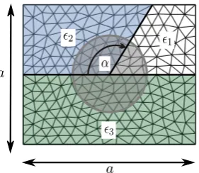
A more complicated setup concerns singularities arising at the contact line between three or more dielectric materials. To avoid additional effects from a non-conformal geometry discretization in a rectangular FIT grid, this setup is investi-gated only for the DG method on a triangular grid. The case of three dielectric wedges, with relative permittivities1=1,
2=80 and3=4 is depicted in Fig. 7. For illustration pur-poses, also an exemplary triangular grid as well as the region used for DG singular basis enrichment are shown. The sin-gularity is given byVs(ρ,ϕ)=ρt9(ϕ), witht≈0.61, cor-responding to a contact angleα=120◦. The boundary
Fig. 7. Domain triangulation and radius of influence for the DG
method with singular basis functions.
max.Error
hmax
DG no cor. DG cor. r=0.03m
DG cor. r=0.05m DG cor.
10-3 10-2 10-1
10-4
10-3
10-2
10-1
1st order
2nd order
Fig. 8. Numerical error for the triple dielectric edge problem using
DG.
5.4 3-D eigenvalue problem with reentrant corner
The last example is the solution of the curl-curl eigenvalue problem for a cavity with reentrant corner. The structure is a hollow, PEC bounded rectangular box (see Fig. 9) (x= 0..1 m, y=0..0.7 m, z=0..0.8 m) in which a PEC rect-angular box is inserted (x=0..0.5 m, y=0..0.35 m, z= 0..0.8 m). In this setup only the first with the singular point corresponding grid edges are corrected. The implementation of an influence region for three-dimensional problems is part of current work. However, in this case both material matrices (Mµ;FIT,M;FIT) have to be corrected to solve the curl curl eigenvalue equation:
M−;FIT1 (CFIT)TM−µ;FIT1 CFIT _
e=ω2_e, (15)
where CFITis the discrete curl matrix of FIT. The convergence
of the first resonance frequency with respect to the grid size is shown in Fig. 10. As observed in the previous examples the standard correction technique () and the new edge correc-tion (∗) improve the accuracy, meanwhile the order of con-vergence remains unchanged.
x y
z
Fig. 9. Arrowplot of the electric field distribution for the eigenvalue
problem.
10-5 10-4
10-5 10-4 10-3 10-2
1/#Gridcells
rel.Errorinf
0
FIT stand. cor.
FIT new cor.
1st order
FIT no cor.
Fig. 10. Convergence of the resonance frequency for the singular
eigenvalue problem using FIT.
6 Conclusions
Two numerical approaches for the simulation of singular field problems have been presented. The first consists in a special modification of the material matrices of FIT, whereas the second represents a DG method with singular basis func-tions. Both methods lead to an immense improvement in nu-merical accuracy in the case of PEC as well as for dielectric edge singularities. Numerical simulations for a number of setups with typical electromagnetic field singularities show, in particular, that the optimal convergence order for regular field problems can be fully recovered when the respective singular corrections are applied within a small but finite re-gion of influence surrounding the singularity.
Acknowledgements. One author (Christoph Classen) wishes to
ac-knowledge the assistance and support of the Deutsche Forschungs-gemeinschaft: GRK 1464.
References
Beilenhoff, K. and Heinrich, W.: Treatment of field singularities in the finite-difference approximation, Microwave Symposium Digest, 1993., IEEE MTT-S International, 2, 979–982, 1993. Castillo, P., Cockburn, B., Perugia, I., and Sch¨otzau, D.: An A
Pri-ori Error Analysis of the Local Discontinuous Galerkin Method for Elliptic Problems, SIAM Journal on Numerical Analysis, 38, 1676–1706, 2000.
Chahine, E., Laborde, P., and Renard, Y.: Crack tip enrichment in the XFEM method using a cut-off function, Int. J. Numer. Meth. Engng., 75, 629–646, 2006.
Classen, C., Bandlow, B., Schuhmann, R., and Tsukerman, I.: FIT & FLAME for Sharp Edges in Electrostatics, in: EMTS 2010 – International Symposium on Electromagnetic Theory, Berlin, Germany, 2010.
Graglia, R. D. and Lombardi, G.: Singular Higher Order Com-plete Vector Bases for Finite Methods, Antennas and Propaga-tion, IEEE Transactions on, 52, 1672–1685, 2004.
Hurd, R. A.: The Edge Condition in Electromagnetics, Antennas and Propagation, IEEE Transactions on, 24, 70–73, 1976. Laborde, P., Pommier, J., Renard, Y., and Salan, M.: High-order
ex-tended finite element method for cracked domains, Int. J. Numer. Meth. Engng., 64, 354–381, 2005.
Meixner, J.: The behavior of electromagnetic fields at edges, Anten-nas and Propagation, IEEE Transactions on, 20, 442–446, 1972.
Melenk, J. M. and Babuˇska, I.: The partition of unity finite element method: Basic theory and applications, Comput. Methods Appl. Mech. Engrg., 139, 289–314, 1996.
Mo¨es, N., Dolbow, J., and Belytschko, T.: A finite element method for crack growth without remeshing, Int. J. Numer. Meth. En-gng., 46, 130–150, 1999.
Mur, G.: The Modeling of Singularities in the Finite-Difference Ap-proximation of the Time-Domain Electromagnetic-Field Equa-tions, Microwave Theory and Techniques, IEEE Transactions on, 29, 1073–1077, 1981.
Olyslager, F.: The behavior of electromagnetic fields at edges in bi-isotropic and bi-anisotropic materials, Antennas and Propaga-tion, IEEE Transactions on, 42, 1392–1397, 1994.
Przybyszewski, P. and Mrozowski, M.: A conductive wedge in Yee’s mesh, Microwave and Guided Wave Letters, IEEE, 8, 66– 68, 1998.
Webb, J. P.: Finite element analysis of dispersion in waveguides with sharp metal edges, Microwave Theory Tech., IEEE Trans-actions on, 36, 1819–1824, 1988.