R E S E A R C H
Open Access
Reduced basis method applied
to a convective stability problem
Henar Herrero
1, Yvon Maday
2,3,4and Francisco Pla
1**Correspondence:
1Dpto. Matemáticas, Univ. Castilla-La
Mancha, Ciudad Real, Spain Full list of author information is available at the end of the article
Abstract
Numerical reduced basis methods are instrumental to solve parameter dependent partial differential equations problems in case of many queries. Bifurcation and instability problems have these characteristics as different solutions emerge by varying a bifurcation parameter. Rayleigh–Bénard convection is an instability problem with multiple steady solutions and bifurcations by varying the Rayleigh number. In this paper the eigenvalue problem of the corresponding linear stability analysis has been solved with this method. The resulting matrices are small, the eigenvalues are easily calculated and the bifurcation points are correctly captured. Nine branches of stable and unstable solutions are obtained with this method in an interval of values of the Rayleigh number. Different basis sets are considered in each branch. The reduced basis method permits one to obtain the bifurcation diagrams with much lower computational cost.
Keywords: Reduced basis; Linear stability; Eigenvalues and eigenfunctions; Bifurcation; Rayleigh Bénard instability; Convective flow
1 Introduction
Bifurcations and instabilities in differential equations are features that allow the explana-tion of many fluid dynamics phenomena in nature and industrial processes [1]. An exam-ple is the Rayleigh–Bénard convection problem [2, 3]. Rayleigh–Bénard and related natu-ral convection phenomena are usual in many industrial applications. For instance, in the formation of microstructures during the cooling of molten metals in computer chips or large scale equipments. The model equations in this case are the incompressible Navier– Stokes equations coupled with a heat equation under the Boussinesq approximation. Here the conductive solution becomes unstable for a critical vertical temperature gradient be-yond a certain threshold and therefore a convective motion sets in, and, depending on boundary conditions and other external physical parameters, new convective patterns oc-cur [1].
All these problems usually need to be solved with numerical methods. To find all the different solutions for the same or different values of the bifurcation parameter and bi-furcations among them specific continuation techniques are required. These techniques are highly developed for ordinary differential equations [4], but are less advanced for par-tial differenpar-tial equations. Some continuation methods consider a perturbation with the eigenfunctions at the bifurcation point in order to find the bifurcated solution, others are
based on the existence of finite dimensional inertial manifolds [5] and projections on this manifold [6], other use proper orthogonal decomposition (POD) [7].
In [8, 9] a Rayleigh–Bénard problem is studied under the perspective of looking for the bifurcation diagrams. The different solutions and successive bifurcations when the tem-perature gradients increase are obtained based on a branch continuation technique. In the study of these bifurcation problems the model of partial differential equations must be solved for lots of values of the bifurcation parameter and a linear stability analysis has to be performed for each solution in order to know its linear stability properties and the succession of bifurcations.
The reduced basis method is a meaningful numerical technique to solve problems of partial differential equation for a large amount of values of the bifurcation parameter with a reduced cost [10–17]. This method consists of the construction of a basis of solutions for different values of this parameter. These solutions are obtained in a preliminary stage with a standard discretization and a greedy selection is applied to them. A further use of a Galerkin method for the reduced basis expansion is implemented.
In this work the reduced basis method is applied as a continuation technique to find the multiple steady solutions and instabilities among them, that appear in a Rayleigh–Bénard convection problem in a rectangle. In [18] the reduced basis method has been applied to this problem to obtain some stable solutions, allowing one to prove the efficiency of the given method to obtain solutions for different values of the parameters. The aim of the present paper is to complete the study of bifurcations with the calculation of the whole bifurcation diagram with all the solutions including the unstable ones, their linear stability, bifurcations among them and the capturing of the bifurcation points. All the steps are solved with reduced basis.
The article is organized as follows. In Sect. 2 we formulate the problem, providing the description of the physical setup, the basic equations and boundary conditions. We de-scribe the numerical stationary problem and the linear stability analysis of the stationary solutions. Section 3 discusses the numerical reduced basis method. Section 4 describes the numerical results. Finally Sect. 5 presents the conclusions.
2 Formulation of the problem
The domain is a rectangle= [0,]×[0, 1] containing a fluid that is heated from below at temperatureT0and on the upper plate the temperature isT1. The equations governing the system are the incompressible Navier–Stokes equations with the Boussinesq approx-imation coupled with a heat equation. The variables present in the problem areuxand
uz, the components of the velocity vector field u,θ the temperature,Pthe pressure,xand
zthe spatial coordinates andtthe time. The magnitudes are expressed in dimensionless form as explained in [18]:
0 =∇ ·u, in, (1)
1
Pr(∂tu+ u· ∇u) =Rθez–∇P+u, in, (2)
∂tθ+ u· ∇θ–uz=θ, in. (3)
Here ezis the unit vector in the vertical direction,Ris the Rayleigh number that measures
modelling, the Prandtl numberPris considered infinite as in [8, 9], then the left hand side term in Eq. (2) can be made equal to zero.
Lateral walls are thermally insulated, non-deformable and free slip. The bottom plate is rigid and the upper surface is non deformable and free slip. These conditions along with the thermal boundaries on the top and bottom plates are expressed as,
u= 0, θ= 0 onz= 0; θ=∂zux=uz= 0 onz= 1, (4)
∂xθ=∂xuz=ux= 0, onx= 0, and onx=. (5)
Equations in problem (1)–(5) are invariant under the symmetry,
γ : (x,z,ux,uz,θ,P)→(–x,z, –ux,uz,θ,P).
Then, ifSis solution of the problem,γSis a solution as well. This solution is said to be in the orbit ofS[19]. We consider solutions in the orbit ofSto be equivalent, so sometimes we restrict ourselves to one single solution in an orbit.
2.1 Stationary equations
The corresponding stationary problem is the following,
∇ ·u= 0, in, (6)
Rθez–∇P+u= 0, in, (7)
u· ∇θ–uz=θ, in (8)
with the boundary conditions (4)–(5). There are results for the existence of solutions in this problem in [20, 21].
This stationary problem (6)–(8) with boundary conditions (4)–(5) is solved numerically with a Newton method for the nonlinear terms [22] and a Legendre collocation [23, 24] for each step in the Newton procedure. In the Newton method an aproximate solution u0
x,u0z,P0,θ0is required at the beginning. This guess solution can be the solution for a
different value of the parameters or the solution for the linear problem. This initial guess is improved by adding to it a small correction as follows:u0
x+u˜x,u0z +u˜z,P0+P˜,θ0+θ˜.
These expressions are introduced into equations (6)–(8) and boundary conditions (4)–(5) where only order one terms in the perturbation fields are kept in the linear approximation. The fields are expanded into Legendre polynomials,
˜ ux=
n i=0 m j=0 aux
ij Li(x)Lj(z), u˜z= n i=0 m j=0 auz
ijLi(x)Lj(z), (9)
˜ P= n i=0 m j=0
aPijLi(x)Lj(z), θ˜= n i=0 m j=0
aθijLi(x)Lj(z), (10)
whereLiis the Legendre polynomial of degreei. The expansions are introduced into the
equations, they are evaluated at the Legendre Gauss–Lobatto points and a linear problem on the coefficientsaux
ij ,a uz
ij,aPij,aθij,i= 0, . . . ,n;j= 0, . . . ,mis solved with a Gaussian
elimina-tion. Then we obtain the solution of the first iteration of the Newton methodu1
u1
z=u0z+u˜z,P1=P0+P˜,θ1=θ0+θ˜. This procedure is repeatedusx+1=usx+u˜x,usz+1=usz+u˜z,
Ps+1=Ps+P˜,θs+1=θs+θ˜until a convergence criterion is satisfied. In particular we have
considered that theL2norm of the computed perturbation should be less than 10–7. Where theL2scalar product and norm are calculated with the Legendre Gauss–Lobatto quadra-ture
f,gGL=
n
l=0
m
s=0
f(xl,zs)g(xl,zs)ρls, (11)
andxl,l= 0, . . . ,n,zs,s= 0, . . . ,m, are the Legendre Gauss–Lobatto points, andρlsare the
Legendre Gauss–Lobatto weights. We have increased the number of polynomials in the Legendre expansion with respect to [18] in order to improve the accuracy of the calcu-lation of the bifurcation points. The criteria to choose an order expansion is the critical Rayleigh number where the bifurcation takes place does not change if we increase further the order expansion. So, in this calculations we have considered expansions of ordern= 35 in thex-direction andm= 13 in thez-direction.
2.2 Linear stability of the stationary problem
Once the stationary solutions (ub,θb,Pb) (x,z) are obtained, the stability of these solutions
is determined by a linear stability analysis as in [8]. In this analysis the stationary solutions are perturbed as follows:
u(x,z,t) = ub(x,z) +u(x,z)exp(σt), (12)
θ(x,z,t) =θb(x,z) +θ(x,z)exp(σt), (13)
P(x,z,t) =Pb(x,z) +P(x,z)exp(σt). (14)
Here superscriptbindicates the corresponding solutions of the stationary problem (6)– (8)–(4)–(5) and the tilde refers to the perturbation. Expressions for the perturbed fields (12)–(14) are introduced in equations (1)–(5) and the resulting equations are linearized. Therefore, if we drop the tildes to simplify notation, we get the following eingenvalue prob-lem:
∇ ·u= 0, in, (15)
Rθez–∇P+u= 0, in, (16)
θ– ub· ∇θ– u· ∇θb+uz=σ θ, in, (17)
together with boundary conditions (4)–(5). The resulting problem is an eigenvalue prob-lem inσ(R). The sign of the real part ofσ(R) determines the stability of the stationary solution. IfRe(σ(R)) < 0 for any eigenvalue of the stationary state, then it is stable, while if there exists a value of σ(R) such thatRe(σ(R)) > 0 then the stationary state becomes unstable. If we nameσ1(R) the eigenvalue with largest real part, asRe(σ1(R)) depends on R, by increasingR,Re(σ1(R)) changes sign at a critical thresholdRc, whereRe(σ1(Rc)) = 0
which separates stable from unstable solutions. The conditionRe(σ1(Rc)) = 0 defines the
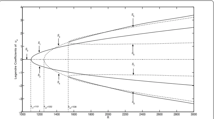
We choose the value of the aspect ratio= 3.495 as in [8, 18] and let the Rayleigh num-berRvary in the interval: [1000; 3000]. In this interval two pitchfork bifurcations and two inverse pitchfork bifurcations appear [18]. In this problem we take into account nine dif-ferent solutions. In the interval [1000; 1102] there is only the zero solutionS0, in the inter-val [1101; 1252] there are two other solutions, three in total,S0,S1andS2, in the interval [1252; 1538] five solutionsS0–S4, and finally in the interval [1538; 3000] nine solutions S0–S8. Therefore solutionS0exists in the interval [1000; 3000], solutionsS1andS2in the interval [1102; 3000], solutionsS3andS4in the interval [1252; 3000] and solutionsS5–S8 in the interval [1538; 3000].
3 Numerical reduced basis method
The numerical method is based on the approximation of all the solutions by the linear combination of some well chosen solutions computed for some particular values ofR, the same ones for every variable: u,θ,P. These values are obtained in a greedy fashion.
3.1 Construction of the reduced basis
The procedure we have implemented in this paper in order to obtain the reduced basis is the pure greedy that is explained next in a inductive way:
– First we fix the solutions we want to calculate and the interval of values ofRwhere these solutions exist.
– We solve numerically the stationary equations (6)–(8) with boundary conditions (4)–(5), with the Newton Legendre collocation method described in the previous section, for different values of the Rayleigh numberRchosen on a subset of the interval, denoted as “trial set”trial. Some values of the Rayleigh number are equidistant, and others are near the bifurcation points. We name the associated solutions(R)≡(u(R),θ(R),P(R)).
– For the first stepi= 1, we choose a value of the Rayleigh number that we nameR1, with its corresponding solution(R1), i.e. in this work it is the smallest value ofRin the interval we consider. We normalize this stationary solution according to theL2 scalar product:
1=
ψ1u= u1 u1L2
,ψ1θ= θ1 θ1L2
,ψ1P= P1 P1L2
,
then we consider a first spaceX1=span{ψ1u} ×span{ψ1θ} ×span{ψ1P}. – We introduce the projection operatorX1u×X1θ×X1PontoX1for theL
2inner
product and consider the approximation (u(1)(R),θ(1)(R),P(1)(R)) = [
X1u(u(R)),Xθ1(θ(R)),XP1(P(R))]for everyR. Note that it corresponds to the product of independent projection operatorsXu
1 ,Xθ1 andXP1. – We evaluate the relative errors of the projections onX1for the velocity and
temperature fieldsu,θ on one side and the pressurePon the other side:
1(1)(R) =(ux(R),uz(R),θ(R)) – (u (1)
x (R),u(1)z (R),θ(1)(R))(L2)3 (ux(R),uz(R),θ(R))(L2)3
and
2(1)(R) =P(R) –P (1)(R)
over any values ofRchosen ontrial. We then chooseR2as follows:
R2=argmax
R∈trial
max
j=1,2 (1)
j (R)
and the corresponding stationary solution is(R2).
– Given stepi, we orthonormalize thei+ 1functions by Gram–Schmidt procedure and we consider thei+ 1space
Xi+1=span{ψ1u, . . . ,ψiu+1} ×span{ψ1θ, . . . ,ψiθ+1} ×span{ψ1P, . . . ,ψiP+1}.
– We introduce the projection operatorXiu+1×Xθi+1×XiP+1ontoXi+1for theL2 inner product and consider the approximation
u(i+1)(R),θ(i+1)(R),P(i+1)(R)=Xiu+1
u(R),Xθ i+1
θ(R),XP i+1
P(R)
for everyR.
– Again, we evaluate the relative errors of the projections onXi+1for the velocity and temperature fieldsu,θ on one side and the pressurePon the other side:
1(i+1)(R) =(ux(R),uz(R),θ(R)) – (u (i+1)
x (R),u(zi+1)(R),θ(i+1)(R))(L2)3 (ux(R),uz(R),θ(R))(L2)3
and
2(i+1)(R) =P(R) –P (i+1)(R)
L2 P(R)L2
,
over any values forRchosen ontrial. We then chooseRi+2as follows:
Ri+2=argmax
R∈trial
max
j=1,2 (i+1)
j (R)
and the corresponding stationary solution is(Ri+2).
– This procedure is repeated until we reach a valueN<card(trial)for which the stopping criteriumj(N)≤10–7,j= 1, 2is satisfied.
Therefore, we obtain the reduced basis{1,2, . . . ,N}and a corresponding discrete
spaceXN≡XuN×X θ
N×XNP. For some solutions we have constructed a reduced basis,
be-sides for other solutions two reduced basis and for other ones three reduced basis, in order to reach the same accuracy for all the solutions. Table 1 shows the number of snapshots used to calculate the reduced basis and the number of elements of the reduced basis for each solution.
Tables 2, 3, 4, 5, 6 present the maximum values of1(j) and2(j) for increasing values of jand the correspondingRparameter in which the maximum value is obtained for the different solutions.
Table 1 Number of snapshots in the trial set for the different reduced basis (RB) for different solution
S1 S3 S3(two sets) S5 S5(three sets)
Table 2 1(j),2(j),j= 1,. . .,Nand the respective Rayleigh numberRin which the maximum takes place for different dimensionsjof the reduced basis space.Ris in the interval [1102; 3000] for solutionsS1
j 1(j)
(j)
2 R
1 0.809 0.236 1102 2 0.085 0.0.009 3000 3 0.008 0.001 1500 4 0.003 4.7·10–4 2200 5 3.3·10–4 6.7·10–5 1110
6 1.1·10–4 1.7·10–5 2700
7 1.7·10–5 2.7·10–6 1900
8 2.8·10–6 4.1·10–7 1800
9 1.8·10–7 1.7·10–8 1300
Table 3 1(j),2(j),j= 1,. . .,Nand the respective Rayleigh numberRin which the maximum takes place for different dimensionsjof the reduced basis space.Ris in the interval [1253; 3000] for solutionsS3
j 1(j)
(j)
2 R
1 0.748 0.588 1253 2 0.056 0.015 3000 3 0.007 0.001 1600 4 0.002 2.5·10–4 2200
5 1.1·10–4 3.5·10–5 1300
6 2.6·10–5 7.4·10–6 2700
7 4.6·10–6 7.5·10–7 1400
8 7.0·10–7 9.6·10–8 1260
Table 4 1(j),2(j),j= 1,. . .,Nand the respective Rayleigh numberRin which the maximum takes place for different dimensionsjof the reduced basis space.Ris in the interval [1253; 1538] for solutionsS3in the upper part of the table andRis in the interval [1538; 3000] for solutionsS3in the
lower part of the table
j 1(j)
(j)
2 R
1 0.354 0.198 1253 2 0.011 0.002 1530 3 6.4·10–4 1.2·10–4 1330
4 6.5·10–5 1.2·10–5 1270
5 1.4·10–6 2.9·10–7 1450
6 2.7·10–7 5.2·10–8 1380
1 0.442 0.412 1539 2 0.018 0.005 3000 3 0.001 2.7·10–4 2100 4 2.4·10–4 5.2·10–5 1700 5 5.9·10–6 8.9·10–7 2600 6 5.5·10–7 2.1·10–7 1900
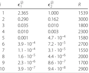
Table 5 1(j),2(j),j= 1,. . .,Nand the respective Rayleigh numberRin which the maximum takes place for different dimensionsjof the reduced basis space.Ris in the interval [1538; 3000] for solutionsS5
j 1(j)
(j)
2 R
1 2.365 1.000 1539 2 0.290 0.162 3000 3 0.035 0.010 1800 4 0.010 0.003 2300 5 0.001 4.7·10–4 1580
6 3.9·10–4 7.2·10–5 2700
7 1.1·10–4 3.1·10–5 1550
8 1.6·10–5 4.4·10–6 2000
9 2.3·10–6 8.6·10–7 1700
Table 6 1(j),2(j),j= 1,. . .,Nand the respective Rayleigh numberRin which the maximum takes place for different dimensionsjof the reduced basis space.Ris in the interval [1539; 1600] for solutionsS5in the first part of the table,Ris in the interval [1600; 2000] for solutionsS5in the second
part of the table andRis in the interval [2000; 3000] for solutionsS5in the last part of the table
j 1(j)
(j)
2 R
1 0.785 0.265 1539 2 0.016 0.006 1600 3 3.1·10–4 8.5·10–4 1560
4 4.4·10–5 1.1·10–5 1545
5 1.1·10–6 3.0·10–7 1585
6 7.2·10–7 2.0·10–8 1541
1 1.154 0.683 1600 2 0.050 0.026 2000 3 0.003 6.6·10–4 1740 4 3.5·10–4 1.2·10–4 1880 5 1.3·10–5 7.8·10–6 1640
6 2.7·10–6 6.4·10–7 1940
7 2.4·10–7 5.0·10–8 1610
1 0.834 0.554 2000 2 0.039 0.022 3000 3 0.002 7.0·10–4 2380 4 3.4·10–4 8.9·10–5 2700 5 1.2·10–5 4.0·10–6 2120 6 2.4·10–6 9.2·10–7 2880 7 1.3·10–7 4.6·10–8 2040
3.2 Galerkin procedure
Once the reduced basis{1,2, . . . ,N}has been calculated, the Galerkin method with
expansions in this basis is implemented to solve the problem (6)–(8) with boundary con-ditions (4)–(5). The nonlinearity of this problem is solved with an iterative Newton pro-cedure, i.e. a linearization of the equations around a previous solution. We start with an approximated solution at iterations= 0, taken e.g. as a previously computed solution at a Rayleigh numberR∗belonging to the trial set, then, at each iteration steps+ 1 we solve the linear problem obtained by linearizing around the previous steps. In practice this proce-dure is equivalent to introduce a perturbation to the steps,
usN+1,x=usN,x+uN,x, usN+1,z=usN,z+uN,z, θNs+1=θNs +θN, PsN+1=PsN+PN,
we want to emphasize that both (usN,x,uNs,z) and (uN,x,uN,z) belong toXNu, bothθNs andθN
belong toXθ
Nand bothPsN andPN belong toXNP.
We then introduce these fields into the equations (6)–(8) and boundary conditions (4)– (5) and linearize with respect to the perturbation. The following problem is obtained (where the tildes have been omitted to simplify notation)
∇ ·uN= –∇ ·usN, in, (18)
RθNez–∇PN+uN= –RθNsez+∇PsN–usN, in, (19)
uN· ∇θNs + usN· ∇θN–θN–uN,z=θNs – usN· ∇θNs +usN,z, in. (20)
Find uN∈XNu andθN ∈XNθ such that:
R
θNvz–
∇uN· ∇v= –R
θNsvz+
∇usN· ∇v, ∀v∈XNu, (21)
uN· ∇θNs + uNs · ∇θN–uN,z
·φ+
∇θN· ∇φ
= –
∇θNs · ∇φ–
usN· ∇θNs –usN,z·φ, ∀φ∈Xθ
N, (22)
we discretize this problem by using expansions in terms of the reduced basis obtained in the previous section, uN=
N
i=1αiψiuandθN =
N
i=1βiψiθ. The integrals are calculated by
using Legendre Gauss–Lobatto integration. Note that our basis of solutions for the velocity are divergence free, and thus the pressure disappears in this formulation.
Each step in the Newton iteration becomes a 2N×2Nalgebraic system of equations:
Ms·ξ= F ⇔
A1 B1 A2 B2
· α β = F1 F2 , where
Ms=
A1 B1 A2 B2
; ξ=
α β
;
Ai∈MN×N, i= 1, 2; Bi∈MN×N, i= 1, 2;
α= (α1, . . . ,αN); β= (β1, . . . ,βN); Fi∈MN×1, i= 1, 2.
Msis a non-singular and well conditioned matrix, condition numbers areO(104) in all the studied cases.
Note that the construction of the matrixMscan be done online very efficiently inO(N3) operations if, during the pre-processing off-line stage, double integrals involving the ele-ments of the reduced basis are computed, we are indeed in the case where the appear-ance of the parameter is outside of the integrals and the problem is only slightly nonlinear (bilinear), during the offline stage the integrals are calculated using the Legendre Gauss– Lobatto quadrature formulas [24].
3.3 Linear stability analysis
Following the Galerkin variational procedure explained in the previous section, the eigen-value problem (15)–(17) described in Sect. 2.2 is presented in its corresponding variational form as follows:
R
θNvz–
∇uN· ∇v= 0, ∀v∈XNu, (23)
uN· ∇θNb + uNb · ∇θN–uN,z
·φ+
∇θN· ∇φ
= –σ
we discretize this problem with the corresponding expansions into the reduced basis, uN=
N
i=1αiψiu andθN =
N
i=1βiψiθ. The eigenvalue problem (23)–(24) is then transformed
into its discrete form as:
Ms·ξ=σB·ξ ⇔
A1 B1 A2 B2
· α β =σ 0 0 0 b · α β , (25)
where b = –(ψθ
i ·ψjθ)Ni,j=1= –IN, whereIN is the identity matrix of sizeN, andA1,B1,
A2,B2,αandβare defined in Sect. 3.2. The discrete eigenvalue problem (25) has a finite number of eigenvaluesσi. As explained in Sect. 2.2 we are interested in the presence of
eigenvalues that have a positive real part. If such eigenvalue exists the solution is unstable otherwise the solution is stable.
3.4 Post-processing
The reduced basis is formed by functions that are not solutions of the Galerkin procedure, indeed these are solutions of a Legendre collocation method. We introduce a rectification post-processing presented in [18], which consists of a change of basis from the reduced basis to the Galerkin solutions on the values ofRof the basis as is explained as follows:
We start by computing the reduced basis Galerkin approximations for all valuesR=Ri,
i= 1, . . . ,N, that are used in the reduced basis construction. This gives us coefficients
uN(Ri) = N
j=1αijψjuandθN(Ri) = N
j=1βjiψjθ. We nameQu(resp.Qθ) the matrix with
en-tries equal toαji (resp.βji). We callSu(resp.Sθ) the matrix with columns equal to the coordinates of u(Ri) (resp.θ(Ri)) in the reduced basisψju(resp.ψjθ),j= 1, . . . ,N. Finally,
we setPu=Su[Qu]–1(resp.Pθ=Sθ[Qθ]–1). This part is done during theoff-linestage and the matrix is stored.
Then for every other values for which we apply the RB Galerkin approximation, we are able to rectify the coefficients as follows: αnew=Puα (resp.βnew=Pθβ) and the post-processed solutions are then
uN
N
i=1
αnew,iψiu, θ N
i=1
βnew,iψiθ. (26)
4 Results and discussion
Figure 1(a) Isotherms and velocity field forR= 1900 for solutionS1and (b)S2; (c) isotherms and velocity
field forR= 1900 for solutionS3and (d)S4
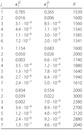
Figure 2(a) Isotherms and velocity field forR= 1900 for solutionS5and (b)S6; (c) isotherms and velocity
field forR= 1900 for solutionS7and (d)S8
4.1 Linear stability analysis
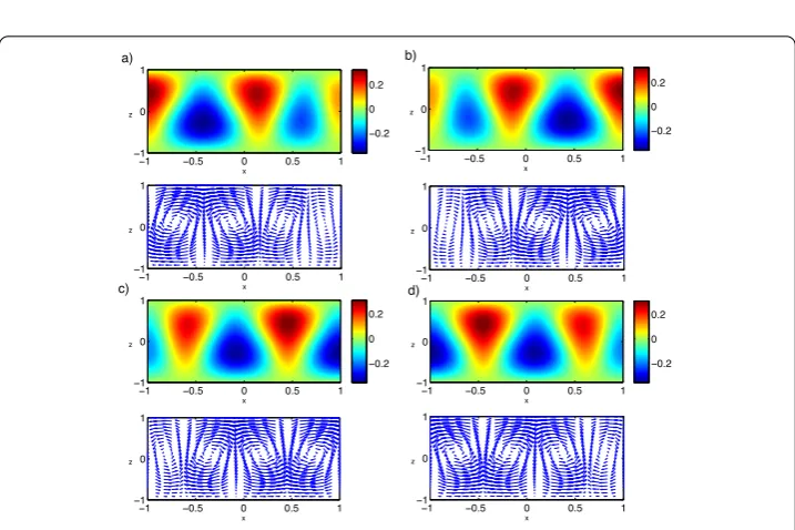
Figure 3(a) Eigenvalue with maximum real part near the bifurcation point. Dashed line for the Legendre solver and solid line for the post-processed reduced basis. (b) Norm of the difference between Re(σ1)
obtained with Legendre collocation and with a post-processed reduced basis method based on Legendre collocation. (c) Norm of the difference between Re(σ1) obtained with Legendre collocation and with a
post-processed reduced basis method based on Legendre collocation divided by the norm of Re(σ1)
obtained with Legendre collocation
first integer where the sign of the real part of the eigenvalue with largest real part changes sign asRincreases. For this reason we say the bifurcation point is correctly captured at Rc3= 1538. But there is an error, with a linear interpolation the value of the bifurcation for Reduced Basis isRc3RB= 1537.5442 and for Legendre collocation it isRc3L= 1537.0860, the relative error isO(10)–4. For both calculations, i.e., Legendre collocation solver and post-processed reduced basis method, the real part of the eigenvalues becomes negative for the same integer value,Rc3= 1538. The same behavior is observed for the rest of the bifurcation points at the values ofRc1= 1101 andRc2= 1252. Therefore, we may conclude that the bifurcation points are correctly captured.
Figure 3(b) shows the norm of the difference between the real part of the eigenvalue with largest real part obtained via Legendre collocation and by a post-processed reduced basis method based on Legendre collocation for solutionsS3 in the interval ofR[1534; 1539] near the bifurcation point atRc3= 1538. This difference isO(10–4) (where both approxi-mations cross near the bifurcation point), increasing as we move away from the bifurcation point. Figure 3(c) shows the norm of the difference between the real part of the eigen-value with largest real part obtained via Legendre collocation and by a post-processed reduced basis method based on Legendre collocation divided by the norm of the real part of the eigenvalue obtained with Legendre collocation for solutionsS3in the interval of R[1534; 1539] near the bifurcation point atRc3= 1538. This difference isO(10–1) except aroundR= 1537 where it isO(1) because the real part of the eigenvalue crosses the axis and becomes zero near this point atRc3L= 1537.0860, for this reason the relative error becomes maximum at this valueR= 1537.
4.2 Capturing the bifurcation points
Once we have calculated all solutions, a plot of the combination of coefficientsa03+a13of the Legendre expansion of the fielduxN as a function of the Rayleigh number is drawn in
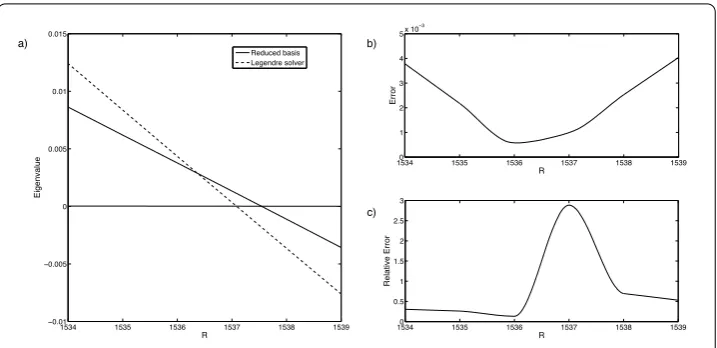
Figure 4Bifurcation diagram where the value of the combination of coefficientsa03+a13of the Legendre
expansion of the fielduxas a function of the Rayleigh number is presented. SolutionsSare calculated by reconstructing all the solutions in each branch by Galerkin approach on the corresponding reduced basis
order to characterise the stationary solutions and its evolution as a function of the Rayleigh number, we present the bifurcation diagram in Fig. 4 with a selection of nonzero coeffi-cientsa03+a13for which the bifurcation diagram is clear. Four bifurcations are observed in this problem. A first pitchfork bifurcation from the zero solution towards solutions with 3 rolls,S1andS2=γS1. A second pitchfork bifurcation from the zero solution towards so-lutions with 4 rolls,S3andS4. Two inverse pitchfork bifurcations fromS3(respectivelyS4) towards non symmetric solutions with the same number of rolls,S5,S6=γS5(respectively, S7andS8=γS7).
The point where different types of solutions intersect or get together is going to be the bifurcation point, where the bifurcation takes place. The first pitchfork bifurcation takes place atR= 1101, where solutionsS1andS2get together. The second bifurcation occurs atR= 1252, where solutionsS3andS4intersect. Finally both secondary inverse pitchfork bifurcations take place atR= 1538, whereS5 andS6 intersect, and whereS7 andS8get together. These bifurcation points are correctly captured with the reduced basis method by plotting the solutions in the bifurcation diagram in Fig. 4. The bifurcations are pitchfork because symmetric solutions appear at those points.
The bifurcation points are also captured with the linear stability analysis as explained in Sect. 4.1.
4.3 Errors on the solutions
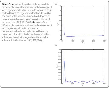
Figure 5(a) Natural logarithm of the norm of the difference between the stationary solution obtained with Legendre collocation and with a reduced basis method based on Legendre collocation divided by the norm of the solution obtained with Legendre collocation without post-processing for solutionS1
in the interval ofR[1101; 3000]; (b) Norm of the difference between the stationary solution obtained with Legendre collocation and with a
post-processed reduced basis method based on Legendre collocation divided by the norm of the solution obtained with Legendre collocation for solutionS1in the interval ofR[1101; 3000]
The errors areO(10–2) far from the bifurcation point, that is already a quite good ap-proximation in comparison with the number of degrees of freedom that have been used in the reduced basis. Near the bifurcation point relative errors increase tillO(10–1) be-cause those points are critical. The solutions cease to exist at these point. The norm of the solutions goes to zero, for this reason a peak appear near the bifurcation point.
With the post-processing explained in Sect. 3.4 the solutions are improved, first, by con-struction the error is zero atR=Ri, for the other values ofR∈[1101; 3000] the maximum
relative error becomesO(10–4) outside the bifurcation point, see Fig. 5(b), where the norm of the difference between the stationary solution obtained with Legendre collocation and with a post-processed reduced basis method based on Legendre collocation divided by the norm of the solution obtained with Legendre collocation for solutionsS1in the interval of R[1101; 3000] is drawn. Near the bifurcation point the relative error increases toO(10–3). The solutions cease to exist at these point. The norm of the solutions goes to zero, and the errors are relative, for this reason a peak appear near the bifurcation point. A better relative error is obtained for the stable part of solutionsS3 in the interval [1539; 3000] where the relative errors areO(10–7) as can be seen in Fig. 6(a). The relative error for the S3unstable solutions are not better thanO(10–4) outside the bifurcation point, near the bifurcation points the relative errors increase toO(10–2), as can be seen in Fig. 6(b). The solutions cease to exist at the bifurcation point. The norm of the solutions goes to zero, for this reason a peak appear near the bifurcation point. Figure 7(a) corresponds to rela-tive errors for solutionS5in the interval [1539; 1600]. Relative errors areO(10–4), except near the bifurcation point, where the error isO(10–3). SolutionsS
Figure 6Norm of the difference between the stationary solution obtained with Legendre collocation and with a post-processed reduced basis method based on Legendre collocation divided by the norm of the solution obtained with Legendre collocation for solutionS3in the interval
ofR(a) [1539; 3000] and (b) [1253; 1538]
third part of solutionS5in the interval [2000; 3000] where the relative errors areO(10–7) as can be seen in Fig. 7(c).
4.4 Advantages of reduced basis method
The reduced basis method is supported by standard discretizations. Theoff-linework for the calculation of the solutions to construct the reduced basis needs these standard meth-ods. But, once the work of the standard method is done, the use of the reduced basis has several advantages.
The pressure variable disappears in the Galerkin approach due to the variational for-mulation and the incompressibility of the fluid (∇ · v= 0). This fact, together with the few modes required for the Galerkin expansion, provides small matrices with the reduced bases discretization. For a single value of the Rayleigh numberRthe size of the matrices that appear after the discretizations is 2016 in Legendre collocation with expansions of or-der 13×35, whereas in the case of the reduced basis with 8 elements the size of matrices is 16. A factor of 126 in the size of the matrices for each value ofR. Legendre collocation matrices are dense by diagonal blocks of size 14×36.
Figure 7Norm of the difference between the stationary solution obtained with Legendre collocation and with a post-processed reduced basis method based on Legendre collocation divided by the norm of the solution obtained with Legendre collocation for (a) solutionS5in the
interval ofR[1539; 1600]; (b) solutionS5in the
interval ofR[1600; 2000]; (c) solutionS5in the
interval ofR[2000; 3000]
of the Rayleigh number the solution must be calculated by increasing slowly the Rayleigh number. For instance, we obtain the first solution in the branch in the interval [1101; 3000] nearR= 1101. To obtain the solution atR= 3000 we need to calculate the solution atR= 1102, take this solution as initial guess forR= 1110 and calculate the solutions increasing the value ofRin steps of 10 tillR= 3000. Sometimes the steps of increase onRcan be larger. So, it is not possible to jump fromR= 1101 tillR= 3000 with Legendre collocation. In the reduced basis this is not the case, the solution can be directly calculated for any value ofR. The reason for this behavior must be that nothing drive the solutions to be attracted by a different branch since there is not unexpected elements in the basis set. Also solutions obtained with reduced basis method are a great help as guess solutions for the Newton method in Legendre collocation. In fact the Legendre solutions necessary to valuate the errors have been calculated solving first with Galerkin reduced basis and taking this solution as initial guess for Legendre.
the branch in the interval [1101; 3000], 190 values ofRand for the branch in the interval [1252; 3000] 175 values ofR. Therefore the whole diagram requires 1314 values ofR. If we take into account symmetries only 511 values ofRare necessary. The problem is nonlinear, if we consider an average of 10 iterations for each problem and we solve the linear systems with a method withO(N2) operations, beingNthe size of the matrices, for each value of Rwe solve the system withO(107) operations for Legendre collocation and withO(103) with reduced basis. Then multiplying by 103values ofR,O(1010) operations for Legendre collocation andO(106) for reduced basis to obtain the whole bifurcation diagram. The off-linenumber of operations of reduced basis requires to solve Legendre for order 10 values of the Rayleigh number, thereforeO(108) operations.
Summarizing, for a single value of the parameterR, theoff-linenumber of operations isO(108), theon-linemaximum number of operations for Legendre collocation isO(109) and for reduced basisO(103). For the whole bifurcation diagram theoff-linenumber of operations isO(108), theon-linenumber of operations for Legendre collocation isO(1010) and for reduced basisO(106).
A significant advantage of solving the eigenvalue problem is provided by the use of a reduced basis, which is due to a large reduction in computational cost. This reduction arises due to the size of the matrices in the eigenvalue problem; in Legendre collocation the size of the matrix is 2016, while using a reduced basis with 8 elements it is only 16. The eigenvalue problem is solved with an adaptation of the implicitly restarted Lanczos method [25]. This method has computational complexityO(N3), whereNis the size of the matrix. Therefore for a fixed value ofRin Legendre collocation the complexity isO(109) whereas for reduced basis it is onlyO(103), six orders lower. For 1000 values of the Rayleigh number Legendre collocation reachesO(1012) and reduced basisO(106). This is reflected in the temporal computational cost, which is 122 s when using Legendre collocation and only it is 6 s using a reduced basis. Therefore the reduction is of a factor of 20 in time.
5 Conclusions
collocation isO(109) and for reduced basisO(103). For the whole bifurcation diagram the off-linenumber of operations isO(108), theon-linenumber of operations for Legendre collocation isO(1010) and for reduced basisO(106). The advantage of solving the eigen-value problem with reduced basis is huge as regards with respect to the large reduction of the computational cost. For a fixed value ofRin Legendre collocation the complexity isO(109) whereas for reduced basis it is onlyO(103), six orders lower. This is reflected in the reduction in the computational cost in time of a factor of 20. There is a startup work in order to calculate the reduced basis, but once this is done, the reduced basis method permits to speed up the computations of these bifurcation diagrams. A study of the eigen-function spaces obtained with reduced basis can be also of interest and it will be addressed in future work.
Acknowledgements
Not applicable.
Funding
This work was partially supported by the Research Grants MINECO (Spanish Government) MTM2015-68818-R, which include RDEF funds.
Abbreviations
RB, reduced basis;R, Rayleigh number;Pr, Prandtl number; GL, Gauss–Lobatto; Re, real part of the eigenvalue; Im, imaginary part of the eigenvalue;Rc, critical Rayleigh number.
Availability of data and materials
Not applicable.
Competing interests
The authors declare that they have no competing interests.
Authors’ contributions
All authors contributed equally and were involved in writing the manuscript. All authors read and approved the final manuscript.
Author details
1Dpto. Matemáticas, Univ. Castilla-La Mancha, Ciudad Real, Spain.2Laboratoire Jacques-Louis Lions, UMR 7598, Sorbone
Universités, UPMC Univ. Paris 06, Paris, France.3Institut Universitaire de France, Paris, France. 4Division of Applied Maths,
Brown University, Providence, USA.
Publisher’s Note
Springer Nature remains neutral with regard to jurisdictional claims in published maps and institutional affiliations.
Received: 14 November 2017 Accepted: 6 April 2018
References
1. Chandrasekhar S, Hydrodynamic and hydromagnetic stability. New York: Dover; 1982.
2. Bénard H. Les tourbillons cèllulaires dans une nappe liquide. Rev Gén Sci Pures Appl. 1900;11:1261–71.
3. Lord R. On convection currents in a horizontal layer of fluid when the higher temperature is on the under side. Philos Mag. 1916;32:529–46.
4. Krauskopf B, Osinga HM, Galán-Vioque J. Numerical continuation methods for dynamical systems: path following and boundary value problems. Berlin: Springer; 2007.
5. Foias C, Sell GR, Temam R. Inertial manifolds for nonlinear evolution equations. J Differ Equ. 1988;73:309–53. 6. Navarro MC, Witkowski LM, Tuckerman LS, Le Quéré P. Building a reduced model for nonlinear dynamics in
Rayleigh–Bénard convection with counter-rotating disks. Phys Rev E. 2010;81(3):036323.
7. Terragni F, Vega JM. On the use of POD-based ROMs to analyse bifurcations in some dissipative systems. Phys D, Nonlinear Phenom. 2012;241(17):1393–405.
8. Pla F, Mancho AM, Herrero H. Bifurcation phenomena in a convection problem with temperature dependent viscosity at low aspect ratio. Phys D, Nonlinear Phenom. 2009;238(5):572–80.
9. Pla F, Herrero H, Lafitte O. Theoretical and numerical study of a thermal convection problem with temperature-dependent viscosity in an infinite layer. Phys D, Nonlinear Phenom. 2010;239(13):1108–19. 10. Almroth BO, Stern P, Brogan FA. Automatic choice of global shape functions in structural analysis. AIAA J.
1978;16:525–8.
11. Noor AK, Balch CD, Shibut MA. Reduction methods for non-linear steady-state thermal analysis. Int J Numer Methods Eng. 1984;20:1323–48.
13. Barrett A, Reddien G. On the reduced basis method. Z Angew Math Mech. 1995;75(7):543–9.
14. Prud’homme C, Rovas D, Veroy K, Maday Y, Patera AT, Turinici G. Reliable real-time solution of parametrized partial differential equations: reduced-basis output bounds methods. J Fluids Eng. 2002;124(1):70–80.
15. Rozza G, Huynh DBP, Patera AT. Reduced basis approximation and a posteriori error estimation for affinely parametrized elliptic coercive partial differential equations. Arch Comput Methods Eng. 2008;15(3):229–75. 16. Noor AK, Peters JM. Bifurcation and post-buckling analysis of laminated composite plates via reduced basis
techniques. Comput Methods Appl Mech Eng. 1981;29:271–95.
17. Noor AK, Peters JM. Multiple-parameter reduced basis technique for bifurcation and post-buckling analysis of composite plates. Int J Numer Methods Eng. 1983;19:1783–803.
18. Herrero H, Maday Y, Pla F. RB (Reduced Basis) applied to RB (Rayleigh–Bénard). Comput Methods Appl Mech Eng. 2013;261(262):132–41.
19. Golubitsky M, Swift JW, Knobloch E. Symmetries and pattern selection in Rayleigh–Bénard convection. Phys D, Nonlinear Phenom. 1984;10:249–76.
20. Lorca SA, Boldrini JL. Stationary solutions for generalized Boussinesq models. J Differ Equ. 1996;124:389–406. 21. Lorca SA, Boldrini JL. The initial value problem for the generalized Boussinesq model. Nonlinear Anal.
1999;36(4):457–80.
22. Herrero H, Mancho AM. On pressure boundary conditions for thermoconvective problems. Int J Numer Methods Fluids. 2002;39:391–402.
23. Bernardi C, Maday Y. Approximations spectrales de problèmes aux limites elliptiques. Berlin: Springer; 1991. 24. Canuto C, Hussaine MY, Quarteroni A, Zang TA. Spectral methods in fluid dynamics. Berlin: Springer; 1988. 25. Bai Z, Demmel J, Dongarra J, Ruhe A, van der Vorst H, editors. Templates for the solution of algebraic eigenvalue