Discovering Quantum Causal Models
Sally Shrapnel
December 28, 2015
I present an Interventionist account of quantum causation, based on the process matrix formalism of Oreshkov, Costa and Brukner (2012), and more recent work by Costa and Shrapnel (2015). The formalism generalises the classical methods of Pearl (2000), and allows for the discovery of quantum causal structure. I show that classical causal structure emerges in certain situations as a special case. I emphasise the crucial role causal discovery plays, in order to distinguish this approach from other recent alternatives.
Contents
1 Introduction. 3
2 Motivating quantum causal models. 6
4 Quantum causal models: a new formalism. 15
5 Discovery and explanation: Bell inequalities. 26
6 The emergence of classical causal structure. 27
1 Introduction.
It is notoriously difficult to apply classical causal modelling techniques to systems involving quantum phenomena. Entanglement correlations seem to defy causal explanation, and it seems near impossible to produce an account that avoids the difficulties posed by non-locality, contextuality, and the measurement problem. In the last thirty years or so, philosophers have advocated a number of fixes, arguing for non-local common causes (Su´arez and San Pedro 2011; Egg and Esfeld 2014),
non-screening o↵ common causes (Butterfield 1992) and “uncommon” common causes (Hofer-Szab´o et al. (2013), Naeger (2015). Others have argued for more exotic solutions such as retrocausation (Evans, Price and Wharton (2013); Evans (2014)) and
superdeterminism (’t Hooft 2009).
All of these approaches share a common theme. Roughly speaking, one starts with quantum correlations, applies classical causal modelling methods, identifies a
contradiction and then decides what has to go. For interventionist accounts, the dilemma is presented as a choice between relinquishing one of two assumptions: the Causal Markov Condition or Faithfulness (no-fine-tuning)1. Whilst these accounts have
much to commend them, unfortunately, they have not led to any kind of consensus. It seems reasonable to advocate a new direction.
The primary motivation for this new direction comes from quantum engineering. Physicists have been producing technologies that harness quantum e↵ects for decades now. Control and manipulation of quantum systems is commonplace in the laboratory, and physicists express the relata and relations that comprise each specific design via the use of quantum circuit diagrams. I think it entirely reasonable to suggest that these
diagrams may represent causal structure. They are acyclic and align with temporal direction. They allow physicists to predict the e↵ect of possible interventions and also to di↵erentiate between e↵ective and ine↵ective strategies. On balance then, there is much to suggest that if one were looking for an interventionist notion of quantum causation, quantum circuit diagrams of engineered systems would be a good place to start.
A number of physicists have recently taken this approach towards causation and produced a generalised notion of quantum circuits.2 Such “circuit models” now pervade the physics literature on quantum causation and the framework I introduce in this paper follows in this same tradition. The starting point for these accounts is not the classical causal modelling formalism we are used to from the philosophical literature. Rather, the starting point is simply the formalism of quantum mechanics, defined in a suitably operational manner. We will take a closer look at these circuit models below. I think this approach to quantum causation represents an important alternative to traditional methods. As we shall see, it provides a new way of analysing the causal structure of the Bell experiments. As mentioned above, the search for causal
explanations for Bell violating correlations has inspired much hair pulling on the part of both philosophers and physicists in the past: here I will present a fresh perspective on this old problem.
One of the founding fathers of classical causal modelling, Judea Pearl, is well aware that his formalism cannot be applied to situations involving quantum mechanics:
... the Laplacian [deterministic] conception is more in tune with human intuitions. The few esoteric quantum experiments that conflict with the
2See, for example, (Gutoski and Watrous (2006), Chiribella, D’Ariano and Perinotti
predictions of the Laplacian conception evoke surprise and disbelief, and they demand scientists give up deeply entrenched intuitions about locality and
causality. Our objective is to preserve, explicate and satisfy - not destroy - those intuitions.(2000), [26]
He chooses to defend his account against various quantum qualms by claiming his causal structure applies only to macroscopic relata:
Only quantum mechanical phenomena exhibit associations that cannot be attributed to latent variables, and it would be considered a scientific miracle if anyone were able to discover such peculiar associations in the macroscopic world (2000), [62]
Whilst one can quibble over what ought to count as “macroscopic”,
experimentalists have pushed hard against the claim that there is some fundamental upper limit at which quantum mechanics simply ceases to apply (see, for example, Eibenberger et al., (2013)). One can no longer sensibly claim that quantum mechanics applies just to the microscopic world. Nor can one sensibly hold that descriptions, explanations and models involving quantum systems are simply bereft of causal content3.
A flurry of recent papers capture something of this new perspective of quantum causation. Bell experiments have been analysed using the causal modelling framework (Wood and Spekkens (2014), Naeger (2015)), dualist versions of causal models have been developed to capture both quantum and classical correlations (Laskey (2007), Henson, Lal and Pusey (2014), Pienaar and Brukner (2014)) and new generalised frameworks suggest quantum causal structure may be fundamental, with classical causal structure emerging as a special case (Oreshkov and Giarmatzi (2015), Costa and
Shrapnel (2015)). It is the latter framework that I shall choose to explicate here.
Whilst all accounts are worthy of exploration, I believe the latter account comes closest to the new direction I am advocating. The aim is to provide a consistent formalism that allows for representation of quantum causal structure, with classical causal structure emerging under certain (decoherent) situations.
The paper is structured as follows: first I motivate the project. Second, I examine exactly what makes Pearl’s classical causal models causal. Third, I introduce the quantum causal modelling framework of Costa and Shrapnel. Fourth, I explain how causal discovery and explanation work in this new framework. Finally, I show how one can recover classical causal structures as a special case. I do not wish to suggest that this is the only possible formulation of a quantum causal model. This is a very new field, and undoubtedly there is much more to be said.
2 Motivating quantum causal models.
I see three distinct reasons to be interested in the proposal I present here. Firstly, the interventionist account of causation was largely inspired by casual modelling in
engineering and the special sciences. As Jenann Ismael puts it, in her usual succinct manner:
Intuitions play almost no role in this [interventionist] literature. The emphasis there is on providing a framework for representing causal relations in science, i.e. a formal apparatus for rendering the deep causal structure of situations...and provides normative solutions to causal inference and judgement problems. (Ismael 2015)[2]
must be possible to distinguish between e↵ective and ine↵ective strategies.
The second motivation for the proposal comes from other recent philosophical work characterising possible quantum causal models. Naeger (2015) and Evans (2015) both advance quantum causal models that take Pearl’s characterisation to be correct, but relax one of the key assumptions, allowing for models with fine-tuned variables. Whilst I think both these accounts are worthy contributions, there is still a concern that they may be, to some extent, throwing the baby out with the bathwater. Causal structures are discovered rather than merely specified. They don’t arise in a conceptual vacuum, but rather evolve in a co-evolutionary manner. As a scientific domain develops and matures, causal explanation and causal discovery typically become two sides of the same coin. Allowing for fine-tuned models, even though the fine-tuning is of a particular kind, disturbs the fine balance between discovery and explanation.
I make this point clearer in the following section. For now, just think of it as reason to look to alternative quantum causal models. The alternative I present here will not try to shoe-horn quantum causal relations into classical ones. Instead, quantum causal structure is seen as fundamental, with classical structure being recovered in an appropriate limit.
Finally, one can also motivate the task of defining quantum causal models as simply providing a new method for gaining some traction on another well-known question: how does the quantum world di↵er from the classical?
3 What makes a classical causal model causal?
due to causes and those that are merely accidental. On this view, causal models are vehicles for learning about the manipulable elements of the world. It is therefore relevant to ask whether causal models are purely of epistemological significance. Many think not. The concept of interventionist causation (at the hands of Woodward and others) has matured beyond an agent-centric approach to one that can be articulated without explicit reference to human action or knowledge. The formal structures of causal modelling are increasingly viewed as devices that give us a handle on the objective, causal structure of the world.4 For those who prefer a modest, less
metaphysically loaded interpretation of causal modelling (see, for example, Woodward (2003) ,Woodward (2007) and Frisch (2014)) the models I discuss here will still be of interest.
A number of authors have contributed in important ways to the development of causal modelling, for example Spirtes et al. (2000) and Woodward (2003), but we will follow the physicists here and use Pearl’s account to focus our discussion. I will spend a little time here explaining the detail of Pearl’s account. This will help the reader
appreciate the problems one encounters when using these methods to characterise quantum causal structure. It will also pave the way for a deeper understanding of the framework presented to account for quantum causal structure.
The causal relata of Pearl’s account are classical random variables X1, .., Xn. It is
assumed that each variable can be associated with a range of “values”: properties that we can unambiguously reveal by measurement or direct observation. Such variables can be binary and used to represent the occurrence or otherwise of an event, can take on a
4See, for example, Ismael (2015). See Price (2007) for an alternative, agent based
finite range of values or have values that are continuous. It is generally assumed that the properties that these values represent are non-contextual (in the sense of quantum contextuality) and exist prior to, and independently of the act of measurement or observation. Ultimately, these values represent the point of contact between the model and the world.
The causal model is formed using an ordered triple hV, G, P ri. Here V is the set of variables, Ga directed graph and P r a joint probability distribution over the variables V. The graph captures the qualitative relationships between the variables, with the nodes of the graph being the variables in V and the arrows between them representing the causal dependencies. Graphs are usually acyclic, in the sense that no path is closed to form a loop; causes cannot be their own e↵ects. Some basic terminology will be useful: a variable A is a ‘parent’ ofB when there is a single arrow from Ato B. In such a situation B is a ‘child’ ofA. A is an ‘ancestor’ of B when there is a ‘directed path’ of several linked arrows fromA to B, in such a case B is a ‘descendant’ of A. The relation of parent to child node, characterised by an arrow, is assumed to represent direct
causation.
The probability measure P is defined over propositions such as A=a, where A is a variable in V with possible value a. P is also defined over conjunctions, disjunctions, and negations of such propositions. Conditional probabilities over such propositions are also consequently well-defined whenever the event being conditioned on is well-defined (Hitchcock 2012).
Pearl was initially motivated by causal discovery rather than explanation. His algorithms were designed to discover causal structure from within probabilistic
possible values, then to exactly specify a probability distribution over all possible combinations of values in the model, one needs kn parameters. Pearl identified that a Bayesian Network provides a possibility for representing such a joint distribution in a more compact form, by identifying conditional independencies and dependencies.
Pearl’s causal models are essentially Bayesian Networks with some additional assumptions, known as the Causal Markov Condition and Faithfulness. A Bayesian Network is a directed acyclic graph (DAG),G, where each node Xi has an associated conditional probability distribution that denotes the dependence of the values of Xi on its parents in the graph, P(Xi|P aG(Xi)). This network represents a joint probability distribution via the rule P(X1, ..Xn) =QiP(Xi|P aG(Xi)). In words, the joint distribution (P), taken over all the variables in the model (V), decomposes over the graph (G) into a collection of smaller conditional probability distributions. This factorisation is crucial to the formal manipulations of the graph that make various causal and statistical inferences possible.
For such probabilistic BN models, directed edges need not convey causal meaning, which is why one needs to assume the Causal Markov Condition and Faithfulness. In Pearl’s own words:
. . . behind every causal conclusion there must lie some causal assumption that is not discernible from the original distribution.” (loc 10189).
An easy way to see this is to consider that there are certain aspects of DAGs that are unidentifiable from observational data alone. Several graph structures can return the same probabilistic conditional independencies. For example:
X Y Z
X Y Z
all capture X?Z|Y. So if we start with purely observational data, and identify the statistical relationship X?Z|Y, we can only construct an equivalence set of graphs. Such graphs are said to be “independence equivalent”, I-equivalent or “Markov
equivalent”. To di↵erentiate between such graphs we need to feed in other assumptions, for example temporal or interventionist information. The important point is that for a probabilistic graph (Bayesian Network) the three structures are equivalent, but for a causal graph (Causal Bayesian network) we must have a means for disambiguating between these possible structures. One can either perform interventions to get to the correct factorisation, or assume statistical constraints.
The Causal Markov Condition states that for a graph G, each variable Xi is
independent of all its non-descendants, given its parentsP a(Xi) in G. One can think of it as a generalisation of Reichenbach’s screening o↵ criteria. That is, it allows the inference from connectedness in the graph to causal dependence. Faithfulness (alternatively stability orno fine-tuning) states that the only conditional
independencies in the distribution P are the independencies that hold for any set of causal parameters D. Another way to put this is that all the independence relations in the probability distribution over the variables in V must be a consequence of the Markov condition. The idea here is that one does not wish to allow for “accidental” independencies that are created when causal paths cancel. Faithfulness licences the inference from unconnectedness in the graph to causal independence.
ensuring the graph is complete. This means each node in the graph is connected to all other nodes in the graph. In such a situation, causal discovery becomes impossible.
Many have argued against this constraint, claiming it is too strong. There are many cases of models of physical systems that appear fine-tuned, despite the fact that intuitively we still wish to call them causal (Cartwright (2001), Andersen (2013)). There is a subtlety that somewhat mitigates this concern however. Recall that causal models are relative to a number of pragmatic choices: the model scope, the range of invariants (background variables we exclude from the model) and the level of detail.5
For any fine-tuned model it will be possible to recover a faithful (stable) model by either changing scope, increasing the level of detail or altering the range of invariance (assuming Pearl’s interpretation below is correct). This is also the case with
Markovianicity: one can fine-grain variable values, increase the scope of the model and look for correlated noise to restore an otherwise recalcitrant causal model to obey the Causal Markov condition. Thus, in classical modelling situations, the Markov condition and Faithfulness guide us toward the most efficacious level to express the causal
structure of a given system and play an indispensable part in causal discovery.6
Pearl suggests two physical facts underpin his claim that BNs that are Markovian
5Invariants is Ismael’s term (2015). The range of invariants is simply the range of
values that the background variables can assume such that the causal relations of the model still hold. Woodward uses the term stability for this concept.
6In some sense, this is part of the real power of Bell’s theorem. Even if one tries all
these options, the statistics one arrives at will nonetheless still be able to violate the
Bell inequality. That is, adding local hidden variables can not alleviate the need for
and Faithful can be interpreted to represent causal structure. Firstly, he assumes the local conditional probability distributions (between parent nodes and their respective child node) encode information about local (in time and space) stochastic mechanisms, where the stochasticity is due to our ignorance about other variables that we do not include in the model. This means that the relationships between the values of parent and child nodes can be expressed as a function Xi =fi(paXi, Ui), where the Ui
represent all the unmodelled influences on the variable values (noise). Crucially, Pearl assumes the Ui to be independent, thus guaranteeing the Causal Markov Condition will hold. On this interpretation the model is probabilistic by virtue of our ignorance about the values of the Ui: the distribution over theUi generates the probability distribution over the model.
The second physical fact that Pearl appeals to states that the act of setting a variable to a particular value (an intervention) can deterministically override the natural causal mechanisms of the model, providing us with new information by disrupting only the local mechanism associated with that node. The intervention is assumed to replace the original causal mechanism with one that determines the child variable valueX =xwith probability 1. Arrows into the intervened variable are broken, and a new probability distribution is associated with the altered graph. Remember, the joint distribution of the undisturbed graph isP(X1, ..Xn) = QiP(Xi|P aG(Xi)), where the product on the right is over all the nodes in the graph. The joint distribution for the altered graph, for example when X3 is set to x, is
P(X1, ..Xn|do(X3 =x) = pp((XX31|P a,...X(Xn3)). Note, it is the factorisation of the joint probability
into local conditional probabilities between parent and child nodes that ensures this manipulation of the graph accurately represents the e↵ect of a localised intervention.
interventionist. The basic axioms of probability theory (positivity, normalisation and additivity) and the causal assumptions of Markovianicity and Faithfulness provide the possibility of testing the model via local interventions.
Pearl has developed two well known algorithms that take as input a list of
conditional independencies (found in a joint distribution over a given set of variables) and return a set of DAG’s as output. The IC algorithm will return a DAG, under the assumptions of Causal Markovianicity, Faithfulness and Causal Sufficiency (no
unmeasured common causes). The IC* algorithm does not require the assumption of causal sufficiency, but will in general only return a partial ancestral graph (PAG): a DAG with any number of undirected edges. These algorithms use observational data only, so the underdetermination of the causal structure can be further reduced if one has access to interventionist data7.
Let us take a step back, and look at two general features of this formalism. Firstly, what are the points of contact between such causal models and the world? Roughly speaking there are two: the data that underlies the variable “values”, and the data that we use to characterise the local interventions. It is worth noting here that both kinds of data are not explicitly included in the final model: it is the axioms of probability theory that get us from the data to the final model.
Secondly, and more importantly (for our purposes at least), is the fact that the application of causal modelling techniques mirrors the iterative manner in which science develops. One does not arrive at a causal model in a conceptual vacuum: typically one does not either just “start with the data”, so to speak, and produce a fully fledged causal model. Nor does one start with a plausible causal structure, according to domain
knowledge and theory, and expect it to perfectly match an empirically derived joint distribution. Rather, the process is one of mutual refinement, where model and theory are developed in a co-evolutionary manner. Pearl’s techniques capture this feature of causal modelling in a mathematically consistent manner. This is also the case for the modelling strategies utilised by Scheines, Glymore and Spirtes (2000).
Recall, a fine-tuned, or non-Markovian model will often imply we have not settled on the best representational strategy for the phenomena in question. Rather than signal a lack of causation, such failures can instead be seen as an indication that more work needs to be done. Searching for hidden variables, fine-graining measurement values, analysing noise models and improving intervention control are all viable options for arriving at an improved model. When the set of variables is expanded, causal relations can come into existence. It is the fit between causal discovery and causal explanation that drives the possibility of such an iterative approach. Valuable work is being done in the field of causal modelling to refine and extend the reach of such techniques.8
For all these reasons, classical causal modelling techniques now take centre stage in much of the current philosophical work involving causation. There is just one problem. They don’t work for systems involving quantum phenomena.
4 Quantum causal models: a new formalism.
It is clear that there are substantial difficulties to overcome in order to clarify a possible candidate for a quantum causal model. The relata of quantum causal models are not going to be variables in the usual classical sense. One can not associate measurement outcomes with properties that exist prior to, and independently of the act of
measurement or observation. The Kochen-Spekker and Bell theorems both confirm the impossibility of ascribing the usual local, non-contextual, classical hidden variables to represent quantum causal structure. This means one can not simply enlarge the variable set, or fine-grain the values, and recover a Markovian, Faithful causal DAG9.
The first change we shall consider then, is the nature of the causal variables.
For classical causal models, one can think of a variable as capturing a possibility space for a collection of spatio-temporally located events. For the quantum case, we can generalise this notion to include events characterised by possible operations inside specific space-time regions.10 Intuitively, one can think of a quantum causal model as a
structure that represents modal information, where the information tells us how what can happen in one space-time region depends on what can happen in another. Such
9See Wood and Spekkens (2014) for a lengthy analysis of Bell experiments using
Pearl’s classical causal methods. The upshot is that one must allow for fine-tuning to produce a causal model that explains such correlations. For Wood and Spekkens (as for
myself) the cost is too great: one loses the ability to discover causal structure.
10The process matrix framework that follows was developed by Oreshkov, Costa and
Brukner (2012), although they did not identify quantum causal models in the sense
reproduced here. Rather they were interested in developing a formalism that could describe the possibility of indefinite causal structure. This framework has been adopted
and modified by Costa and Shrapnel (2015) as a possible candidate for producing
quantum causal models. The issue of indefinite causal structure, whilst interesting, will
not be addressed here. In the present work I assume that operations take place in a
modal information is accessed by considering the possibility of (i) local choices of operations associated with each space-time region, and (ii) physical systems passing information between each space-time region. The nodes correspond to the space-time regions where we can perform our interventions, and the edges correspond to the transferring physical systems that carry information from one region to another. As such, the connecting physical systems play a similar role as the local mechanisms of Pearl’s causal models, that determine the functional relationship between parent and child nodes.11
Circuit diagrams are a representation of just this kind of structure. There are two distinct varieties of diagram we need to distinguish here. The first is the familiar kind, as depicted in Neilsen and Chuang’s famous textbook (Nielsen and Chuang 2000). Wires are associated with quantum systems. The state of these systems can be
manipulated into superposition states: logic gates represent a physical interaction that changes the state of the quantum system in a predictable manner.
X | iout
| iin
As the system passes between the gates, it is assumed that the state does not change. Thus the wires in these diagrams represent the identity map, 1. The gates are assumed to e↵ect a unitary evolution of the state, and can be switched on and o↵ at various times (in the diagram, the box marked “X”). Measurements are typically pushed to the far right of the circuit, and represent the outcomes of the computation.
The second kind of circuit is a generalisation of this basic structure, to include a variety of di↵erent possible experimental situations in a more abstract manner. The
11In the language of quantum information, an edge corresponds to aquantum channel
wires still represent the quantum state of a physical system, but the state can now change between the gates. This is reflected by associating the more general completely positive map with the wire. Intermediate nodes no longer represent single possible gates, but rather are place holders for a variety of possible interactions, including non-deterministic ones (to allow for the possibility of measurements). It is this latter, more general, kind of circuit that will form the basis for the quantum causal model formalism. The details of these circuits will become clearer below as we examine the mathematical structure in more detail and see some specific examples.
For now, the picture to keep in mind is simply one where nodes correspond to the space-time regions where we perform our interventions, and the edges correspond to the transferring physical systems that carry information from one region to another.
How does one go about attaching probabilities to such a structure? The assignment of probabilities to quantum data is usually via the familiar Born Rule: P(j) =T r(Oj⇢), where Oj here is the relevant measurement operator and ⇢the density matrix. We shall need to generalise this rule, but for now it is enough to recall that this will shape how we attach probabilities to objects in the model.
Typically, we associate measurements with operators, or more generally POVM’s.12
However, in many cases we wish to encode not just the outcome of a measurement, but also the transformation to the state that occurs during the measurement process. Mathematically, the most general object one can associate with such a quantum operation is a trace-non-increasing completely positive map (CP map)13. We can
12Recall a POVM is a Positive Operator Valued Measure: a set of positive,
semi-definite matrices that sum to the identity.
associate each region with sets of such CP maps. Ultimately, these CP maps will perform the same formal function as the variable values in the classical case, they provide us with the possibility space associated with each node. A particular set of CP maps together can characterise a quantuminstrument. Essentially an instrument represents one out of a number of ways we can interact with the system. For example it may represent a choice of measurement setting, basis, preparation etc. We shall see that such instruments ultimately represent the possible interventions we can perform to test the causal structure of the model.
The mathematical arena of the CP map is the Hilbert space we associate with the space-time region. One can decompose this space into the tensor product of two
subsystems: one associated with the incoming system, HAI, and one with the outgoing
system, HAO. The CP map, denotedM
AIAO
j , is a linear map that sends states in the input Hilbert space HAI to states in the output Hilbert space HAO. Each use of an
operation in a given space time region will be associated with one out of a possible set of outcomes, and we label thesej = 1, ...., n. We can thus consider that each outcome induces a particular transformation in the state from input to output, and this is captured by the CP map associated with that outcome. For example, for region A and outcome j we denote the associated CP map as MA
j :L(HAI)!L(HAO).
A
j k
HAO HBI
B
HAI HBO
In the diagram above, the nodes A and B represent distinct spatio-temporal regions. The Hilbert space associated with these regions is defined by the tensor
product of the spaces associated with the incoming and outgoing systems, for example,
j, and the outcome of the operation at B is represented ask. One can generalise to cases that include multiple incoming and outgoing edges, as we shall see in the examples below.
We can now consider how to associate probabilities with such operations. If a CP map is performed on a quantum state ⇢, then MA
j(⇢) describes the updated,
non-normalised state in the case that outcome j is observed. The probability to observe this particular outcome is given by the Born Rule: P(MA
j) = T r[MAj (⇢)]. If we assume our list of possible outcomes (j = 1, ..., n) is complete, then the sum of all CP maps will be trace preserving and completely positive. Another way to put this is that we are guaranteed to have a legitimate probability distribution: with certainty at least one outcome j will occur. Such a complete set of CP maps constitutes a particular
instrument.14
We now have a description that can link a probability distribution to a single node. The next step is to consider how to extend this to provide a valid distribution over all the nodes in the graph. First let us consider the simple case of two nodes, labelled A and B, as in the diagram above. We assume that the joint probability, P(Mj,Mk), for a pair of maps to be realised should be independent of the particular set of possible CP
14Whilst the definition of a quantum instrument is relatively intuitive in the case of
finite, discrete systems, it can become more complicated for the continuous case. See (Davies and Lewis 1970) for a more formal definition of a quantum instrument that
captures both situations. The generalisation to the continuous case does not threaten
any of the arguments made here. Roughly, one can think of an instrument as a
generalisation of a POVM that also captures transformations to the sysytem: for a one
maps associated with either A or B: the joint probabilities must reflect a kind of non-contextuality of the CP maps. That is, what kind of instrument we choose to use atA should not e↵ect the kind of instrument we choose to use at B.15 Characterising a
probability distribution over a pair of outcomes, j and k, that correspond to maps P(Mj), P(Mk) is not entirely straightforward. We will need to make use of a little mathematical trick. I give a simplified account in the footnote below, but see Oreshkov, Costa and Brukner (2012) for the full story.16
The details of why we represent the CP maps in this form are not crucial for our purposes, we just note that as a result, we can represent the probabilities for two measurement outcomes in di↵erent space-time regions A and B, as a bilinear function of the corresponding CJ operators:
P(MA
j,MBk) = T r[WAIAOBIBO(MjAIAO ⌦M BIBO
k )] (1)
15This is essentially the no-signalling condition.
16The trick involves representing a CP map as particular kind of matrix using an
isomorphism called the Choi-jamiolkowski isomorphism (CJ). First consider that a CP
map can also be represented as a matrix on the tensor product Hilbert space,
Mj 2(HAI ⌦HAO), where I Mj 0. We denote the complete set of outcomes
j = (1....m) for a given operation as {MAIA0
j }mj=1. Each element of this set is positive
and, by virtue of the tensor product structure, if we trace over the output space, we will
recover the identity on the input space. The CJ matrix corresponds to a particular
form of linear map, defined as MAIAO
j :=
⇥
I⌦M(| +ih +|)⇤T, where | +iis a
Where WAIAOBIBO is a matrix in L(HAI ⌦HAO ⌦HBI ⌦HBO), known as the process matrix. This matrix can be generated by taking the tensor product of all the maps representing connections between the nodes, written in their CJ form. One can think of equation 1 as a further generalisation of the Born Rule, with the process matrix
analogous to a quantum state and the object (MAIAO
j ⌦M
BIBO
k ) analogous to an operator.
With respect to our causal model, the process matrix W encodes possible connections between the two space time regionsA,B. This is easiest to see by considering a less trivial concrete example, involving three nodes and two wires. Imagine one is given three boxes, labelled A, B and S, connected by wires, labelled (i) and (ii). Each box comes equipped with a set of levers to represent possible
instruments, and a readout associated with possible outcomes. By gathering statistics that relate outcome results with respective instrument settings, one can produce a W matrix. The aim is to use this information to di↵erentiate between the two possible situations depicted below.
A B
S
(i) (ii)
(1) Bipartite entangled state: common cause.
A B
S
(2) Direct cause structure.
Figure (1) depicts the familiar Bell scenario: the production of an entangled
bipartite state. We shall refer to this as the common cause structure. Figure (2) depicts the direct transfer of a quantum physical system between three distinct locations: a direct causal structure. The process matrix ought to be able to tell us which of the two circuits has been implemented.
In order to depict these two structures as quantum causal models, we first need to associate an input and output space for all three nodes. In this simple case we need an input and output space for each of A and B (labelled HAI,HAO,HBI,HBO). For S we
need one input space (HSI) and two output spaces (HSO1,HSO2)17.
First let us use these example networks to compose a process matrix for each case from the terms in each example. For a known causal structure, one can compose the process matrix from the tensor product of terms corresponding to the various
components of the network. For example, the process matrix for the common cause structure will compose as (1) Wc =⇢SI ⌦TSO1AI
1 ⌦T
SO2BI
2 ⌦1AOBO. Where ⇢SI is the
input state at S, TSO1AI
1 is the CJ matrix representing the channel from S toA,T2SO2BI
is the CJ matrix representing the channel from S toB, and1AOBO is the identity map
on the output states at A and B. In a similar manner, one can compose the process matrix for the direct cause structure as (2) Wd =⇢AI ⌦TAOSI
1 ⌦T2SO1BI ⌦⇢SO2 ⌦1BO.
Here⇢AI represents the input state at A, TSO1AI
1 represents the connection from A toS,
TSO IBI
2 represents the connection between S and B, ⇢SO2 represents that component of
the output space of S that in this case we trace out, and 1BO is the identity on the
output of BO.
These examples show that, generally speaking, it is easy enough to decompose the process matrix into tensor products of various circuit components if we already know the structure being described. The crucial question, of course, is whether one can go in the other direction. Can one reconstruct the correct W matrix from the observed statistics of outcomes at A, B and S? Furthermore, is it possible to di↵erentiate between the two cases depicted and thus discover the causal structure of the network from that data alone?
Interestingly, if one has enough statistical data one can construct a unique (minimal) circuit from a given process matrix W. As with the classical case, if one doesn’t require the minimality assumption, an equivalence class of models can be recovered. So how much data is enough? This is related to the notion of
“informationally complete” sets of measurements (POVMS): a single quantum state can be discovered correctly given such a set of measurements (Prugovecki 1977). One can generalise the notion of informational completeness to extend to sets of CP maps and situations that model multiple systems.18 As with the classical case, causal discovery in
this more general setting is intimately related to the characterisation of an ideal intervention. We now turn to consider a plausible quantum analogue.
Interventions in such a model follow naturally from the fact that we associate nodes with the space of possible local CP maps. An intervention can thus be characterised by choosing a particular kind of possible local instrument from within the local space-time region. For example, this may correspond to a choice of measurement setting, basis
18This is due to the possibility of process and state tomography (Nielsen and Chuang
2000), and can be formally extended to the case of process matrices (Costa and
choice, or preparation. This will define the specific sets of CP maps associated with the node. To ensure that such interventions are, in the relevant sense, local, we can demand that the interior of a region can interact with the rest of the universe only through the region’s input and output spaces: it is closed to any traffic not explicitly expressed via edges in the model. This means particular kinds of interventions on a single space-time region will arrow-breaking in a similar manner to the classical case. One can conceive of freely choosing the particular kinds of instrument to use within a given region in a manner that is statistically independent of any other, unconnected space-time region in the model. As with the classical case, one can implement a randomisation procedure here to provide an appropriately agent-independent notion of “free choice”.
Let us look at our specific example to make this connection to the classical idea of intervention a little clearer. Imagine trying to di↵erentiate between the two cases we mentioned above. One can distinguish between these two structures by performing an arrow breaking intervention at A. An obvious example of such an intervention is the set of CP maps that realises a state preparation at A.
How is it possible to di↵erentiate between these two structures using such an intervention? Remember, the causal structure of these models, in general, identifies e↵ective strategies for changing distributions over outcomes, rather than particular outcomes themselves. Thus, one cannot intervene at A and produce a change in the distribution over outcomes at B for the common cause structure in figure 2a.
Consequently, there is no direct causal relation between A and B. However, one can
5 Discovery and explanation: Bell inequalities.
Recall Pearl’s quote from section 1:
... The few esoteric quantum experiments that conflict with the predictions of the Laplacian conception evoke surprise and disbelief, and they demand
scientists give up deeply entrenched intuitions about locality and causality. Our objective is to preserve, explicate and satisfy - not destroy - those
intuitions.(Pearl 2000)[26]
It seems that it is possible to preserve the spirit of these intuitions and explicate a version of quantum causation that observes a well defined notion of both locality and causality. The causal models presented here are local in the sense that they support causal inference via local interventions and also in the sense that the physical systems responsible for the connections are assumed to observe relativistic constraints. They are
causal because they allow us to di↵erentiate between e↵ective and ine↵ective strategies. On this view, contra to the intuitions that so-called “steering” phenomena a↵ord, one cannot intervene at A and produce a change at B for the common cause structure in figure 2a. Thus, in this picture there is no direct causal relation between A and B, in accordance with Woodward’s intuitions regarding Bell correlations (Woodward 2007) and also in accordance with the no-signalling principle. However, one can intervene at S and make changes at both A and B, validating the common cause structure depicted.
Interestingly, for these quantum causal structures there is also an intuitive notion of fine-tuning. Consider once again the direct cause structure depicted in Figure 2. For the case where the set of instruments realised at S were to range over a set that only produced maximally entangled states, for example the four Bell states: |00ip+|11i
2 , |00ip|11i
2 ,
|01ip+|10i
2 ,
|01ip|10i
2 . Recall, one output system will be traced over and one output
be maximally mixed. This means that regardless of the choice of instrument, one will never see a causal relation between S and B. There is an independence in the data that is not reflected in the true causal structure, just as in the classical case of fine-tuning. As with the classical case, one can demand that it is an assumption of the framework that one does not allow for such fine-tuned models.
6 The emergence of classical causal structure.
I believe one of the key virtues of this approach is that quantum causal structure is seen as fundamental, with classical structure emerging as a special case. There are three main reasons why I think this ought to be the case. Generally speaking, the most prolific users of both classical and quantum theory - physicists - take it as given that quantum theory is the more fundamental theory of the two (Copenhagenism aside). Secondly, there is a well described dynamics that takes one from quantum structure to classical structure under certain circumstances (decoherence)19. Finally, one can
provide examples of how the quantum models described in this paper can also apply to classical structures as a special case.
A classical model can be characterised by considering sets of instruments that are restricted to be diagonal in the product basis of the Hilbert space associated with each node. Recall each node is associated with a total Hilbert space, generated via the tensor product of the Hilbert spaces associated with each incoming and outgoing edge. One can ask why we might be restricted to the use of only these particular instruments, and here we can fall back on the usual arguments from decoherence theory. It is the
19See Zurek (2014) and Schlosshauer (2010) for an introduction to the foundational
contingent features of the unknown environment, interacting with the instrument and determining the pointer basis for that node, that so limits our choice of instrument.
Decoherence theory provides tools to explain how and when quantum probability distributions change to classical probability distributions. Thus, it seems likely that we can co-opt these techniques to help explain the relationship between quantum and classical causal models. As yet, this feature of quantum causal models has not been studied in any detail, so for now I will just give a flavour of what might be expected. One of the important lessons of this field is that the quantum-classical boundary is mobile: it can be shifted smoothly by varying particular experimental parameters. In principle then, one ought to be able to model a gradual and continuous shift between a quantum and classical causal model. It would seem that this could be done by
explicitly adding in another quantum node to account for a decohering environment. On such a view, the structure and statistical constraints that we typically associate with classical causal models are in fact a special subset of the deeper causal structures that quantum correlations allow for. Recall Pearl’s picture of the physical story that underlies causation: deterministic relations between events, characterised by local mechanisms, with the probabilities entering by virtue of our ignorance of all the facts. We face quite a di↵erent picture here. Typically, the quantum circuit model carries with it the underlying assumption that evolution of states is unitary and probabilities enter by virtue of fundamental indeterminism.20 One can, in principle, always recover a
quantum causal model from a classical one by expanding the variable set to include a decohering environment. As such, the deeper physical interpretation of quantum causal
20This assumption is justified by the Stinespring Dilation theorem (Nielsen and
models will be hostage to the same concerns as any interpretation of quantum theory. Choosing to be a Many Worlder, a Collapsican, or a Bohmian will not invalidate anything I have said here.
7 Conclusions.
Summing up, I have presented an interventionist account of quantum causation based on the process matrix formalism of Costa and co-workers. I outlined three reasons to consider this proposal: (i) by interventionist lights, the existence of engineered quantum systems and the representational resources that accompany their explication and design flag the possibility of quantum causal structure, (ii) current classical causal modelling methods fail to produce a solution that retains the possibility of causal discovery, and (iii) such a project may ultimately cast new light on the question of how the classical and quantum worlds di↵er.
Acknowledgements
Appendix A
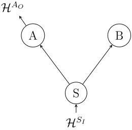
To distinguish between the two particular causal structures depicted in Figure (1) and Figure (2), one can limit the necessary instruments to simple state preparation and measurement options. This will enable one to recover the correct process matrices for each case. Whilst other possible instruments exist, they do not add any additional useful information in this particular case. For clarity, we can alter the figure to include all the required Hilbert spaces:
HAO
A B
S
HSI
(1) Bipartite entangled state: common cause.
A B
S
HAI
HsO2
(2) Direct cause structure.
Let us label the measurement outcomes a, band s respectively for each node, and the choice of instrument x, y and r, respectively for each node. The appropriate instruments to use at each node will be:
MsS|r =ESI
s ⌦⇢ SO1
r ⌦⇢ SO2
r (2)
MaA|x =EAI
a ⌦⇢AxO (3)
MB
b|y =EbBI (4)
where, for example, ESI
s is the POVM element corresponding to measurement outcome s, and ⇢SO1
r represents a state preparation at SO1 that depends on r. Recall, a POVM is a set of positive semi-definite matrices that sum up to identity. The informationally complete sets of POVM’s and preparations to use in this instance would be the six projectors associated with the Pauli matrices. The projectors associated with both the POVMs and preparation procedures would therefore be:
Ea1 =Eb1 =Es1 = 3E1 =|x+ihx+|
Ea2 =Eb2 =Es2 = 3E2 =|x ihx |
Ea3 =Eb3 =Es3 = 3E3 =|y+ihy+|
Ea4 =Eb4 =Es4 = 3E4 =|y ihy |
Ea5 =Eb5 =Es5 = 3E5 =|z+ihz+|
⇢x1 =⇢y1 =⇢r1 =|x+ihx+|
⇢x2 =⇢y2 =⇢r2 =|x ihx |
⇢x3 =⇢y3 =⇢r3 =|y+ihy+|
⇢x4 =⇢y4 =⇢r4 =|y ihy |
⇢x5 =⇢y5 =⇢r5 =|z+ihz+|
⇢x6 =⇢y6 =⇢r6 =|z ihz |
(6)
Recall, the W matrix for the common cause and the direct cause structures will decompose di↵erently as:
Wc =⇢SI ⌦TSOAI
1 ⌦T
SO2BI
2 ⌦1AOBO (7)
Wd =⇢AI ⌦TAOSI
1 ⌦T
SO1BI
2 ⌦⇢SO2 ⌦1BO (8)
If one has access to the above instruments at each node then one can recover the termsTSOAI
1 and T
SO2BI
2 from the gathered statistics. This means that one can calculate
the conditional probability over all the nodes according to the generalised Born rule: From equation (1):
P(a, b, s|x, y, r) =T r⇥W(MAI
a|x⌦M AI
b|y ⌦M BI
s|r)
⇤
(9)
(10)
case. For the common cause P(a, b, s|x, y, r) = P(s)P(a|r)P(b|r). For the direct cause P(a, b, s|x, y, r) =P(a)P(s|x)P(b|r). The direction of the channels tell us the
appropriate conditionals to use. Each of the conditional probabilities corresponds to the probability for the child to detect a POVM element given the state of the parent, transmitted through the corresponding channel.
References
Andersen, Holly. 2013. “When to Expect Violations of Faithfulness and Why it Matters” Philosophy of Science 80(5): 672-683.
Butterfield, J. 1992 “David Lewis Meets John Bell.” Philosophy of Science 59(1).
Cartwright, N. and Jones, M. 1991. “How to hunt quantum causes.” Erkenntnis 35: 205-231.
Cartwright, N. 2001. “What Is Wrong with Bayes Nets?.” The Monist 84:242-264.
Cavalcanti, Eric G, and Raymond Lal. 2014. “On Modifications of Reichenbach’s Principle of Common Cause in Light of Bell’s Theorem.” Journal of Physics A: Mathematical and Theoretical 47(42):424018.
Chaves, R., Majenz, C. and Gross, D. 2015. “Information-theoretic implications of quantum causal structures.” Nature Communications 6: 5766.
Chiribella, G., D’Ariano, G. M. and Perinotti, P. 2009. “Theoretical Framework for Quantum Networks.” Physical Review A.80: 022339.
Costa, F and Shrapnel, S. 2015. “Quantum Causal Models”
Davies, E. and Lewis, J. “An operational approach to quantum probability.” Comm. Math. Phys.17: 239-260.
Eberhardt, Frederick. 2013. “Direct Causes and the Trouble with Soft Interventions.”
Erkenntis 79(4): 755-777.
Egg, Matthias, and Michael Esfeld. 2014. “Non-local Common Cause Explanations for EPR.” European Journal for Philosophy of Science 4:181–196.
Eibenberger, S., Gerlich, S., Arndt, M., Mayor, M. and T¨uxen, J. 2013. “Matter-wave interference with particles selected from a molecular library with masses exceeding 10,000 amu.” Phys. Chem. Chem. Phys. 15: 14696.
Evans, P. W. and Price, H. and Wharton, K. B. 2013. “New Slant on the EPR-Bell Experiment” Brit. J. Phil. Sci.64:297-324.
Evans, P. W. 2014. “Retrocausality at no extra cost”, Synthese.
Evans, P. W. 2015. “Quantum causal models, faithfulness and retrocausality.” arxiv: 1506.08925.
Frisch, Mathias. 2014. “Causal Reasoning in Physics” Cambridge University Press Cambridge.
Glymore, Clark. 2006. “Markov properties and Quantum Experiments” InPhysical Theory and its Interpretation eds. Demopoulos, W. and Pitowsky, I. Springer. 117:126.
Gutoski, G. and Watrous, J. 2006 “Toward a General Theory of Quantum Games.” In
Hausman, Daniel M, and James Woodward. 1999. “Independence, Invariance and the Causal Markov Condition.” The British Journal for the Philosophy of Science 50: 521–583.
Henson, J. and Lal, R. and Pusey, M. F. 2014. “Theory-independent limits on
correlations from generalized Bayesian networks” New Journal of Physics 16: 113043
Hitchcock, C. 2012. “Probabilistic Causation” In The Stanford Encyclopedia of Philosophy.ed. Edward N. Zalta.
Hofer-Szab´o, G´abor, Mikl´os R´edei, and L´aszl´o E Szab´o. 2013. The Principle of the Common Cause. Cambridge: Cambridge University Press.
Ismael, J. 2015 “How do causes depend on us? The many faces of perspectivalism”
Synthese: 1-23.
Ismael, J. forthcoming. “Against Globalism about Laws”. In Experimentation and the Philosophy of Science, eds. Bas van Fraassen and Isabelle Peschard, University of Chicago Press.
Laskey, K. 2007. “Quantum Causal Networks” Proc. AAAI Spring Symp. on Quantum142
Leifer, M. S., and Robert W Spekkens. 2013. “Towards a Formulation of Quantum Theory as a Causally Neutral Theory of Bayesian Inference.” Physical Review A
88(5):052130–052138.
N¨ager, P. M. 2015. “The causal problem of entanglement” Synthese, 1-29
Oreshkov, O., Costa, F. and Brukner, C. 2012. “Quantum correlations with no causal order.” Nature Communications 3: 1092.
Oreshkov, O. and Giarmatzi, C. 2015. “Causal and causally separable processes.” http://arxiv.org/abs/1506.05449v2
Pearl, Judea. 2000. Causality: Models, Reasoning and Inference. Cambridge: Cambridge University Press.
Pienaar, Jacques, and Caslav Brukner. 2014. “A Graph-Separation Theorem for Quantum Causal Models.” arXiv:1406.0430.
Price, H. 2007. “Causal Perspectivalism” In Causation, Physics, and the Constitution of Reality: Russell’s Republic Revisited eds. Price, H. and Corry, R. Oxford
University Press. 10: 250-292
Prugovecki, E. 1977. “Information-Theoretical Aspects of Quantum Measurement.”
International Journal of Theoretical Physics 16(5): 321 - 331.
Ried, K., Agnew, M., Vermeyden, L., Janzing, D., Spekkens, R. W., Resch, K J. 2015. “A quantum advantage for inferring causal structure.” Nature Physics 11: 414 - 420.
Russell, Bertrand. 1912. “On the Notion of Cause.” Proceedings of the Aristotelian Society 13:1–26.
Schlosshauer, Maximilian A. 2010. Decoherence and the Quantum-To-Classical Transition. Berlin: Springer.
Shrapnel, Sally. 2014. “Quantum Causal Explanation: Or, Why Birds Fly South.”
Shrapnel, Sally and Milburn, Gerard. 2015. Unpublished Manuscript.
Spirtes, Peter, Clark Glymour, and Richard Scheines. 2000. Causation, Prediction, and Search. Cambridge, Mass.: MIT Press.
Su´arez, Mauricio, and I˜naki San Pedro. 2011. “Causal Markov, Robustness and the Quantum Correlations.” InProbabilities, Causes and Propensities in Physics, ed. Mauricio Su´arez, 173–193. Dordrecht: Springer.
’t Hooft, Gerard. 2009. “Entangled quantum states in a local deterministic theory.” arxiv: 0908.3408
Timpson, Christopher.2013. “Quantum Information Theory and the Foundations of Quantum Mechanics.” Cambridge University Press.
van Fraassen, Bas C. 1982. “The Charybdis of Realism: Epistemological Implications of Bell’s Inequality.” Synthese 52:25–38.
Wood, C. J. and Spekkens, R. W. 2014 “The lesson of causal discovery algorithms for quantum correlations: Causal explanations of Bell-inequality violations require fine-tuning” New Journal of Physics 17(3):033002.
Woodward, James. 2003. Making Things Happen. A Theory of Causal Explanation. Oxford: Oxford University Press.
———. 2007. “Causation with a Human Face.” In Causation, Physics, and the
Constitution of Reality, eds. Huw Price, and Richard Corry, 66–105. Oxford: Oxfo rd University Press.