Trajectory-Linearization Based Robust Model Predictive Control
for Constrained Unmanned Surface Vessels
Liang Wang, Tairen Sun, Xin Yu
Jiangsu University, Department of Electrical and Information Engineering, Xuefu st.301,Zhenjiang, Jiangsu province, China
e-mail: [email protected]
http://dx.doi.org/10.5755/j01.itc.45.4.13678
Abstract. In this paper, a trajectory-linearization based robust model predictive control (MPC) approach is proposed for unmanned surface vessels (USVs) with system constraints and disturbances. The trajectory linearization technique is used to translate a continuous-time nonlinear model of vessels into a linear time-varying predictive model and to decrease the complexity of nonlinear MPC. The control scheme includes a linear feedback control and a MPC term, where the former ensures the real trajectory being contained in a tube centered at the reference trajectory, and the later ensures asymptotic stability of the nominal system. The effectiveness of the designed control is analyzed theoretically and illustrated by simulation results.
Keywords: trajectory linearization; unmanned surface vessel; model predictive control; robustness.
1. Introduction
The trajectory tracking and path-following of unmanned surface vessels (USVs) attracted more and more attention, due to applications in military and civil, including resource detection, environmental surveillance, maritime rescue, reconnaissance, and mine countermeasures [1-5]. However, disturbances from wind, waves, and ocean currents severely affect the stability of USVs and bring difficulties to controller design. Therefore, how to design robust tracking control for surface vessels is of great signi-ficance. Up to now, many robust tracking controllers for vessels have been obtained based on sliding-mode control [6-8], H∞ control [9-11], neural-network
control [12-18], fuzzy control [19] and disturbance observer -based control [20]. However, the state and input constraints are seldom considered in these approaches. Factually, the control powers of USVs are limited and the states are constrained due to collision avoidance and limited working space. Thus, it is valuable to design robust control for USVs with state and input constraints.
Model predictive control (MPC) is well known for its advantage of receding horizon optimization, robus-tness and its ability in actively handling constraints, and has been successfully applied in petro-chemical, robotics, and so on [21, 22]. Nowadays, for cons-trained uncertain systems, robust model predictive control (RMPC) has been obtained mainly based on
min-max MPC [23, 24] and constraint tightening approaches [25, 26]. In these results, the constraints are satisfied in receding horizon optimization, which is online solved for all possible realization of uncer-tainties. However, this possibly brings infeasibility and conservatism of the online-solved optimal control problem. The tube-based MPC described in [27, 28] mitigates the disadvantages of RMPC in [23-26], since its decision variables include not only the usual con-trol sequences, but also the initial state of the nominal model at each optimization iteration. However, the current results on tube-based MPC are mainly based on discrete-time models, while unmanned surface vessels are usually modeled as continuous-time linear system. Therefore, the continuous-time non-linear system-based tube RMPC is considered as the approach to design a control law for constrained USVs.
In this paper, a trajectory-linearization based tube MPC is proposed for USVs to track desired trajectories. A linear time-varying predictive model is constructed by trajectory linearization [29, 30] of the vessel’s continuous-time nonlinear model. The use of linear time-varying model not only decreases computational complexity of nonlinear MPC, but also maintains the model precision. For simplicity, only kinematic model with additive disturbance is considered in this paper.
paper. Trajectory linearization of vessel’s nonlinear system is constructed and the robust control invariant set for the error system are established in Section 3. Section 4 is devoted to tube-based MPC design. At last, simulations are stated in Section 5 and conclu-sions are presented in Section 6.
Notation. Denote n
R as the n-dimensional Euclidean
space. Define C(0) as the neighborhood of zero with
being the radius. The symbols and ⊖ denote
Minkowski sum and difference, respectively.
2. Problem statement
The kinematic model of the unmanned surface vessel is described as
cos sin 0
sin cos 0 +d( )
0 0 1
x u
y v t
r
, (1)
Where [x y ]T R3 denotes the position
and heading of vessel in the earth-frame coordinate
system; 3
[u v r]T R
represents the
surge, sway, and yaw velocities in the vessel-frame coordinate system, respectively; d t( ) denotes the
system disturbance. The sets and are two
closed sets and both contain zero as their interior point.
The objective of this paper is to design tube-based RMPC for (1) such that the state [ , , ]x y T tracks the
command signal [ , , ]T
com com com
x y .
3. Main results
3.1. Trajectory linearization
In this section, the trajectory linearization approach is adopted to convert the vessel’s nonlinear system into a time-varying linear system.
From (1), the nominal rate for a predetermined trajectory
x t( ) y t( ) ( )t
T iscos ( ) sin ( ) 0 ( ) sin ( ) cos ( ) 0 ( )
0 0 1 ( )
u t t x t
v t t y t
r t
(2)
with
1 2 1
0 1 0
( ) ( )
,
( ) ( ) ( )
( ) d d ( ) d com
x t x t
d
x
a t a t a t
x t x t
dt
(3)
where x t( ) y t( ) ( )t T and
x t( ) y t( ) ( )t
Tare calculated in equation (3) by passing command
state
Tcom com com
x y into a twice-order,
low-pass, command filter. The states ( )x t and x t( ) in (3)
represent the estimations of xcom( )t and its derivative,
respectively. In (3), 2
1( ) ,
d n diff
a t , ad2( )t 2n diff, ,
with being the damping ratio, n diff, being the
natural frequency, which determines the bandwidth of the filter. y t( ) and ( )t can be obtained similarly as
( )
x t .
Define
[ ]T ( ) ( ) ( )T ( ) ( ) ( )T
x y
e e e x t y t t x t y t t (4)
and
u v r
T u t( ) v t( ) r t( )
Tu t( ) v t( ) r t( ) .
T (5)Taking linearization of equation (1) along
x t( ) y t( ) ( )t
T and
u t( ) v t( ) r t( )
T, we canobtain the following linearized error dynamics
( ) ( ) ( ).
x x
y y
e e u
e A t e B t v w t
e e r
(6)
Define [ ]T
x y
e e e e ,
u v r
T. Then,the system (6) can be rewritten in the following form
( ) ( ) ( )
eA t eB tw t , (7)
where
0 0 ( ) sin ( ) ( ) cos ( ) ( ) 0 0 ( ) sin ( ) ( ) cos ( ) ,
0 0 0
u t t v t t
A t u t t v t t
cos ( ) sin ( ) 0 ( ) sin ( ) cos ( ) 0 ,
0 0 1
t t
B t t t
(8)
( ) n
e t R is the state of system (7); ( )t Rm is the control of system (7); w t( )Rn denotes lumped disturbances containing linearization errors and
system disturbances, which satisfies
( ) { nw|
w t w R w wmax} for all t ≥ 0.
From the constraints on and in (1), the dynamics (7) is subject to state and control constraints
Tx y
and
Tu v r
with
and being compact sets containing zero as their interior point.
3.2. Robust control invariant set
The nominal system of (7) can be stated as
( ) ( ) ,
e A t eB t (9)
where is the nominal control input of (9).
Suppose that there exist ( )K t such that the matrix
( ) ( ) ( )
A t B t K t is stable.
Define T T T
x y x y x y
ee e e e e e e e e .
If the control law for (7) is designed as
( ) = ( ) ,
K t e e K t e
(10)
then, based on (7)-(10), the dynamics of the error system is
,
x x
y y
e e
e A e w
e e
(11)
where A[ ( )A t B t K t( ) ( )]diag a
11 a22 a33
, whichsatisfies that a11<0, a22<0, a33<0.
Lemma 1. Denote max{a11,a22,a33} 0, then the
set
2 max
: |
2 (2 )
w e e F
is a robust
control invariant set for the controlled uncertain system (11), where
( ) T / 2
F e e e and is a designed positive constant.
Proof. Taking time derivative of F and substituting
(11), yields
.
T T T T
Fe Aee we ee w (12)
Using Young’s inequality 1
2 2
T T T
e w e e w w
,
then, we can further obtain the following result
2 max
2 max
1
( / 2)
2 1
( / 2)
2 1
=(2 ) .
2
T T
T
F e e w w
e e w
F w
(13)
From (13) we can see that the derivative of F is guaranteed to be less than zero, as long as the following expression holds
2 max
.
2 (2 )
w F
(14)
Therefore, the set
2 max
: |
2 (2 )
w e e F
is a robust control invariant set for the controlled uncertain system (11).
Proposition 1. If (0)e e(0) , w and
K t( ) , then ( )e t e t( ) holds for all
t > 0, where ( )e t and ( )e t are the states of system
model (10) and (11), respectively.
4. Tube-based MPC
4.1. Construction of Tube-based MPC
Denote ( , , ( ), ( ))e t t e tk k as the movement of the nominal system (9) from the initial time tk and initial state ( )e tk for a control signal. Then the cost function
( ( ), ( ))
J e t t of the receding horizon optimization
problem is formulated as follows:
( ( ), ( )) k p ( ( ), ( ))
k t T
k t
J e t
l e d( (k p)),
G e t T
(15)
where ( , ) 1( ), G( ) 1
2 2
T T T
l e e Qe R e e Pe ;
Q, R and P are positive definite symmetric matrices;
0
p
T is defined as the prediction horizon.
Assume there exist a matrix K such that
( )
K t K . Then, the system constraints for the
nominal system in the MPC can be constructed as follows:
( )
e ⊖.. [ ,t tk kTp); (16)
( ) V V
⊖K.. [ ,t tk kTp); (17)
(k p) f
e t T ⊖. (18)
Hence, the set of feasible control sequences at sampling time tk can be defined by
U ( ( ))
{ ( ), [ , ) | ( ) , ( ) , [ , ), ( ) }.
N k
k k p
p p f
e t
t t T V e
t t T e t T
(19)
It is assumed that is small enough to ensure that interior( ) and K interior( ), and the terminal constraint set f satisfies:
1) A f f, f ⊖,K f ⊖K,
f is closed and 0 f; (20)
2) f is a positively invariant set for
( ) ( )
e A t eB t Ke; (21)
3) [G l e Ke ]( , ) 0, e f. (22)
Remark 1. If e and e e , the e and
can be concluded. If and e e
hold, from K e e( ), we can conclude that
In the conventional continuous-time MPC for the nominal model, the optimal problem at sampling time
k
t is defined by
*
*
( ( )) min{ ( , ) | ( ) U ( ( )), [ , )},
( ) arg min{ ( , ) | ( ) U ( ( )), [ , )}.
k N k
k k p
k N k
k k p
V e t J e e t
t t T
t J e e t
t t T
(23)
Compared with the conventional optimal control problem, the new optimization problem in tube MPC involves the initial state. This is permissible because the initial state in the optimal problem is now not equal to the current state ( )e tk of the system, which cannot be instantaneously changed, but a parameter of the control law. The new optimal control problem is defined by
0
0
* *
0 0 ,
0
* *
0 0 0
,
0
( ( )) min{ ( , ) | ( ) U ( ( )), [ , ), ( ) ( ) }, ( ( ), ( )) arg min{ ( , ) | ( ) U ( ( )), [ , ), ( ) ( )
k e N k
k k p k k
k N k
e
k k p k k
V e t J e e t
t t T e t e t
e t J e e t
t t T e t e t
}.
(24)
If the function * 0
( ),
e t tt is defined as
* *
0 0 0 0 0 1
*
* *
0 0 1
( , , ( ), ( )), [ , )
( ) ,
( , ,k ( ),k ( )), [ ,k k )
e t t e t t t t
e t
e t t e t t t t
(25)
then according to Proposition 1, we can obtain
*
0
( ) ( ) , .
e t e t tt (26)
Based on the above analysis, the tube MPC for system (7) can be stated as:
* *
0 0 +1
( ) ( ) ( )( ( ) ( )), [ , ) , k 0,1, 2, .
k k
t t K t e t e t t t t
(27)
4.2. Stability analysis of the proposed control
Definition 1.
1. XN { ( ) |e t0 e t( ), ( )0 e t0 e t( )0 ,UN( )e
is not empty};
2. The robust control invariant set is robustly asymptotically stable for system (7) controlled through (25) with XN as the
region of attraction if, for all admissible disturbance, a) dist e t( ( ), ) 0 as t
for all e t( )0 XN and b) for all >0, 0
such that, for all e t( )0 C(0) , then
( ) (0)
e t C for all tt0.
Theorem 1. Suppose the optimization problem (24) is
feasible at sampling time tk .Then, 1) The optimization problem (24) is feasible for all
sampling time tn with n>k;
2) The optimal value function satisfies
1
* * * *
0 0 1 0 0
2 2
* *
( ( )) ( ( ))
k ( ( ) ( ) ) ;
k
k k
t
Q R
t
V e t V e t
e d
(28)3) The set is asymptotic stable for the controlled continuous-time nonlinear system
( ) ( ) ( )
eA t e B t w t with ( )t *( )t *
1
( )( ( ) ( )), [ ,k k )
K t e t e t t t t for a sufficiently
small sampling time interval δ>0.
Proof.
1) It is assumed that at sampling time tk, an
opti-mal solution * * *
0 0
( ( ), e tk ( , ( ), , e tk t tk kTp)) to problem (24) exists and is found. Therefore, the state
* 0
( , ( ), , k k k p)
e e t t t T and the input *( ; ( ), ,e t0* k tk
)
k p
t T , [ , tk tkTp] satisfy the constraints
(16)-(18). When applied to the nominal system (9), the
state will be driven from *
0( )k
e t to *
0
(k p, , k ( ), k
e t T t e t *( )) f.
Since the state of nominal system at time
1
k k
t t
is * *1 0
(k , ,k ( ),k ( ))
e t t e t and e t(k1)
* *
1 0
(k , ,k ( ),k ( ))
e t t e t holds, e t(k1, ,t e tk 0*( ),k *( )) is a feasible choice of initial state of the optimization (24) at time tk1. Since
* 0
(k p, ,k ( ), ( ))k
e t T t e t
f
, K f ⊖ K and f is positively
invariant for e A t e( ) B t Ke( ) . Then, at sampling
time tk1, the control input ( ) on [tk1,tk1Tp) may be chosen as
* *
0 1
1
( , , ( )), [ , ] ( )
( , , , ( )), [ , ).
k k k k p
k p k p k p
t e t t t T
Ke t T t T t T
(29)
Therefore, the feasibility of the optimal control problem (24) with constraints (16)-(18) at time tk
implies its feasibility for all sampling time tn with
n>k.
2) The optimal value of the objective functional at time tk can be written as
2 2
* * * *
0 0
2
* *
0
( ( )) ( ( ) ( ) )
+ ( , , ( ), ( )) .
k p
k
t T
k Q R
t
k p k k P
V e t e d
e t T t e t
Since at sampling time tk1, a feasible control input can be chosen as (29), then the value of the objective function at sampling time tk1 is
1 1 1 1 2 2 1 1 2
1 1 1
2 * * * 0 0 2 * * 0 2 2 1 1 ( ( ), ( )) ( ( , , ( ), ( )) ( ) ) + ( , , ( ), ( )) ( ( , , ( ), ( , , ( ))) + ( , , ( )) ) + ( ( , , , ( )) ( ) ) k p k k p k k t T
k k Q R
t
k p k k P
t T
k k k k Q
t
k k R
k Q R
V e t
e t e t d
e t T t e t
e t e t t e t
t e t d
e t
1 1 1 2 1 2 * * * * *0 0 0 0
2
* *
0
2 2
*
0 1 1 1
1 + ( , , , ( )) ( ( )) ( ( , , ( ), ( , , ( ))) ( , , ( )) ) + ( ( ; ( ), , ) ( ) ) + ( , , k p k p k k k p k p t T t T
k p k p P
t
k t k k k k Q
k k R
t T
k k k p Q R
t T
k p k p
d
e t T t T
V e t e t e t t e t
t e t d
e e t t t T d
e t T t T
2 , ( )) P (31) 2 * 0(k p, ,k ( ),k k p) .
P
e t T t e t t T
From *
0
(k p, ,k ( ),k k p) f
e t T t e t t T and
inequa-lity (22), we can obtain the following result
1 2 1 2 * 0 2 2 *0 1 1 1
( , , , ( ))
( , , ( ), )
( ; ( ), , ) ( ) .
k p k
k p k p P
k p k k k p P
t T
k k k p Q R
t T
e t T t T
e t T t e t t T
e e t t t T d
(32)Therefore, the following results can be obtained from (31)-(32),
1 * 1 * * 0 0 2 * * * 0 0 2 * * 0 ( ( )) ( ( )) ( , , ( ), ( , , ( ))) ( , , ( )) . k k k k tk k k k Q
t
k k R
V e t
V e t
e t e t t e t
t e t d
(33)At last, the result (28) can be concluded from the
fact that * * *
0( 0(k 1)) ( (k 1)) V e t V e t .
3) It can be easily seen from (28) that the sequence
* * 0 0
{V (e t( )), kk 0,1, 2,} is monotonic non-increasing
and with 0 being a lower bound. Thus, *
0
{V ( )}
converges to some non-negative value as k tends to infinity. Then, from (28) and the convergence of
* * 0 0
{V (e t( )), kk 0,1, 2,}, the following result can be
concluded
1 * * * 2
0 0
2
* *
0
* * * *
0 0 0 0 1
lim sup ( , , ( ), ( , , ( )))
( , , ( ))
lim ( ) lim ( ) 0.
k
k t
k k k k Q
t k
k k R
k k
k k
e t e t t e t
t e t d
V e t V e t
(34)Then, we can obtain
lim sup ( ) 0.
t e t (35)
Since 0 lim inf ( ) lim sup ( )
t e t t e t
and (34),
(35) hold, we can get the following result
lim ( ) 0.
t e t (36)
Since ( )e t e t( ) and ( )e t 0ast, the set is robustly asymptotic stable for the controlled nonlinear uncertain system (7).
5. Simulation results
In this section, the effectiveness of the proposed control law is illustrated by simulation. Based on (3), we set 0.5 , n diff, 4 , xcom2 , ycom2 ,
com
/ 4 and ( (0), (0), (0)) (0,0,0)x y , then we
get [ ( ), ( ), ( )]x t y t t T and [ ( ), ( ), ( )]u t v t r t T.
In the linearization (7) of the system (1), the lumped disturbance is denoted as ( ) [0.1sin(0.1 ) w t t
0.1sin(0.1 ) 0.05sin(0.1 )]t t T . The constraints to the
system (7) are described as: x 2.5, y 2.5,
1.2, and 1 u 6, 1 v 3,-1 r 1. In the simulation, we set K=-0.5I, P=0.5I, Q=I and R=0.2I. We set the sampling time as δ=0.1. The terminal state constraint in the MPC is chosen as { |e e PeT 0.06}.
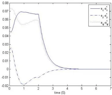
Based on these designed parameters, the control for the system (7) is executed by using MATLAB. The simulation results are showed in Fig. 1-Fig. 3, where Fig. 1 presents the error between the state of
Figure 2.The tracking of command signals for the vessel
Figure 3.The designed control ( , , )u v r for the surface vessel
(ex ey e) and ( ,e e ex* y*, *) , Fig. 2 depicts the tracking of command signals xcom2 , ycom2 ,
com
/ 4. From Fig. 1-Fig. 3, we can get the
effectiveness of the designed tube-based robust MPC, including input and state constraints satisfaction and robustness of the closed-loop system.
6. Conclusions
In this paper, we have proposed a trajectory-linearization-based robust model predictive control (RMPC) for unmanned surface vessels with system constraints and disturbances. In the proposed RMPC, the linear feedback control ensured the real trajectory contained in a tube of trajectory of a nominal system, while the MPC guaranteed the asymptotical stability of the nominal system. We have also provided theoretical analysis and simulation results to illustrate the effectiveness of the proposed control.
Acknowledgments
This work was supported by the National Natural Science Foundation of China (No. 61503158), Natural
Science Foundation of Jiangsu Province (No. BK20130536, No. BK20130533), Scientific Research Foundation for Advanced Talents by Jiangsu Univer-sity, and the Priority Academic Program Development of Jiangsu Higher Education Institutions.
References
[1] K. D. Do, Z. P. Jiang, J. Pan. Global partial-state feedback and output-feedback tracking controllers for underactuated ships. Systems and Control Letters, 2005, Vol. 54, No. 10, 1015-1036.
[2] W. Dong, Y. Guo. Global time-varying stabilization of underactuated surface vessel. IEEE Transactions on
Automatic Control, 2005, Vol. 50, No. 6, 859-864.
[3] M. Wondergem, E. Lefeber, K. Y. Pettersen, H. Nijmeijer. Output feedback tracking of ships. IEEE
Transactions on Control Systems Technology, 2011,
Vol. 19, No. 2, 442-448.
[4] P. Švec, A. Thakur, E. Raboin, B. C. Shah, S. K. Gupta. Target following with motion prediction for unmanned surface vehicle operating in cluttered environments. Autonomous Robots, 2014, Vol. 36, No. 36, 383-405.
[5] D. C. Gandolfo, L. R. Salinas, A. S. Brandão, J. M. Toibero. Path following for unmanned helicopter: an approach on energy autonomy improvement.
Information Technology & Control, 2016, Vol.45,
No. 1, 86-98.
[6] H. Ashrafiuon, K. R. Muske, L. C. McNinch, R. A. Soltan. Sliding mode tracking control of surface vessels, IEEE Transactions on Industrial Electronics, 2008, Vol. 55, No. 11, 556-561.
[7] T. R. Sun, H. L. Pei, Y. P. Pan, H. B. Zhou, C. H. Zhang. Neural network-based sliding mode adaptive control for robot manipulators. Neurocomputing, 2011, Vol. 74, Issue 14-15, 2378-2384.
[8] R. Yu, Q. Zhu, G. Xia, Z. Liu. Sliding mode tracking control of an underactuated surface vessel. Control
Theory and Applications, 2012, Vol. 6, No. 3, 461-466.
[9] M. R. Katebi, M. J. Grimble, Y. Zhang. H∞ robust control design for dynamic ship positioning. IEE
Proceedings-Control Theory and Applications, 1997,
Vol. 144, No. 2, 110-120.
[10] Y. P. Pan, Y. Zhou, T. R. Sun, M. J. Er. Composite adaptive fuzzy H∞ tracking control of uncertain nonlinear systems. Neurocomputing, 2013, Vol. 99, 15-14.
[11] Y. P. Pan, M. J. Er, D. P. Huang, T. R. Sun. Practical adaptive fuzzy H∞ tracking control of uncertain nonlinear systems. International Journal of
Fuzzy Systems, 2012, Vol. 14, No. 4, 463-473.
[12] M. Chen, S. S. Ge, B. V. E. How, Y. S. Choo. Robust adaptive position mooring control for marine vessels.
IEEE Transactions on Control Systems Technology,
2013, Vol. 21, No. 21, 395-409.
[13] Z. Zhao, W. He, S. S. Ge. Adaptive neural network control of a fully actuated marine surface vessel with multiple output constraints. IEEE Transactions on
Control Systems Technology, 2014, Vol. 22, No. 4,
1536-1543.
[14] Y. P. Pan, H. Y. Yu, E. J. Er. Adaptive neural PD control with semiglobal asymptotic stabilization guarantee. IEEE Transactions on Neural Networks and
[15] T. R. Sun, H. L. Pei, Y. P. Pan, C. H. Zhang. Robust wavelet network control for a class of autonomous vehicles to track environmental contour line.
Neurocomputing, 2011, Vol. 74, No. 17, 2886-2892.
[16] T. R. Sun, H. L. Pei, Y. P. Pan, C. H. Zhang. Robust adaptive neural network control for environmental boundary tracking by mobile robots. International
Journal of Robust and Nonlinear Control, 2015,
Vol. 23, No. 2, 3097-3108.
[17] Y. P. Pan, T. R. Sun, H. Y. Yu. Peaking-free output-feedback adaptive neural control under a nonseparation principle. IEEE Transactions on Neural Networks and
Learning Systems, 2015, Vol. 26, No. 12, 3097-3108.
[18] Y. P. Pan, Y. Q. Liu, B. Xu, H. Y. Yu. Hybrid feedback feedforward: an efficient design of adaptive neural network control. Neural Networks, 2015, Vol. 76, 122-134.
[19] Y. P. Pan, D. P. Huang, Z. H. Sun. Backstepping adaptive fuzzy control for track-keeping of underactuated surface vessels. Control Theory and
Applications, 2011, Vol. 28, No. 7, 907-914.
[20] Y. Yang, J. Du, H. Liu, C. Guo, A. Abraham. A trajectory tracking robust controller of surface vessels with disturbance uncertainties. IEEE Transactions on
Control Systems Technology, 2014, Vol. 22, No. 4,
1511-1518.
[21] S. J. C. Lins Barreto, A. G. Scolari Conceicao, C. E. T. Dorea, L. Martinez, E. R. De Pieri. Design and implementation of model-predictive control with friction compensation on an omnidirectional mobile robot. IEEE/ASME Transactions on
Mechatronics, 2014, Vol. 19, No. 2,467-476.
[22] Monteriù, A. Freddi, S. Longhi. Nonlinear decentralized model predictive control for unmanned
vehicles moving in formation. Information Technology & Control, 2015, Vol. 44, No. 1, 89-97.
[23] D. Limon, T. Alamo, F. Salas, E. F. Camacho. Input to state stability of min-max MPC controllers for nonlinear systems with bounded uncertainties.
Automatica, 2006, Vol. 42, No. 5, 797-803.
[24] E. C. Kerrigan, J. M. Maciejowski. Feedback min-max predictive control using a single linear program: robust stability and the explicit solution. International
Journal of Robust and Nonlinear Control, 2004,
Vol. 14, No. 4, 395-413.
[25] L. Magni, G. De Nicolao, R. Scattolini, F. Allgower. Robust model predictive control for nonlinear discrete-time systems. International Journal of Robust and
Nonlinear Control, 2003, Vol. 13, No. 3-4, 229-246.
[26] L Chisci, J. A. Rossiter, G. Zappa. Systems with persistent disturbances: predictive control with restricted constraints. Automatica, 2001, Vol. 37, No. 7, 1019-1028.
[27] D. Q. Mayne, M. M. Seron, S. V. Rakovic. Robust model predictive control of constrained linear systems with bounded disturbances. Automatica, 2005, Vol. 41, No. 2, 219-224.
[28] S. Yu, C. Maier, H. Chen, F. Allgower. Tube MPC scheme based on robust control invariant set with applications to Lipschitz nonlinear systems. System
and Control Letters, 2011, Vol. 62, No. 62, 2650-2655.
[29] Y. Liu, J. Jim Zhu, R. L. Williams, J. Wu. Omni-directional mobile robot controller based on trajectory linearization. Robotics and Autonomous Systems, 2008, Vol. 56, No. 5, 461–479.
[30] Y. Xue, C. Jiang. Trajectory linearization control of an aerospace vehicle based on RBF neural network.
Journal of Systems Engineering and Electronics, 2008,
Vol. 19, No. 4, 799-805.