Volume 01, No. 10, October 2015
P
age
56
Experimental Investigation and Process Variable Optimization of
Abrasive Flow Machining Process for Satellite Component
Arun Raj
*, George Oommen
**& Akhil K V
**** P.G Scholar, Department of Mechanical Engineering, Sree Buddha College of Engineering, University of
Kerala, India
** Scientist / Engineer ‘SF’, CS&SC-CF, CFP/CSC/LPSC-ISRO, Kerala, India
*** Assistant Professor, Department of Mechanical Engineering, Sree Buddha College of Engineering,
University of Kerala, India
ABSTRACT:
Abrasive flow machining (AFM) is an advance machining process which is used to machine complex shape and is used to deburr, remove recast layer and radius surfaces. This research uses a developed abrasive flow machine and an experiment employing abrasive flow machining was conducted on plunger body fabricated on stainless steel SS 446. In this research AFM parameters such as abrasive particle size, concentration, and number of cycles were optimized. In the optimization work surface roughness and edge radius are taken as output. L9 orthogonal array based upon Taguchi method has been preferred for experimental design and Grey Relational Analysis used for multiple response optimization. Deburring action of abrasive flow machining process on plunger body was also observed by means of photographic analysis
Keywords: Abrasive Flow Machining, deburr, grey relational analysis, optimization, surface finish, Taguchi method.
INTRODUCTION
Volume 01, No. 10, October 2015
P
age
57
high edge radius for a given set of parameter combination was developed using combined Taguchi method and Grey Relational Analysis.
ABRASIVE MACHINING AND NON-TRADITIONAL PROCESSES
Abrasive machining is a material removal process that involves the use of abrasive cutting tools. There are three principle types of abrasive cutting tools according to the degree to which abrasive grains are constrained. They are bonded abrasive tools, coated abrasive tools and free abrasives. The conventional machining processes normally involve the use of energy from electric motors, hydraulics, gravity, etc. and rely on the physical contact between tools and work components. On the contrary, advanced material removal processes utilize energy from sources such as electrochemical reactions, high temperature plasma, high velocity jets and loose abrasives mixed in various carriers etc. Burrs are sharp edges resulting from cutting and stamping operations. Although usually small in size, burrs can cause assembly problems, interfere with fluid flow, and are a common cause of worker injury. Burrs can also cause increased stresses and subsequent fatigue failure of the part. Abrasive flow machining is an advanced machining process used to improve surface finish and edge conditions. The abrasive particles in the media grind away, rather than shear off, the material. There are three types of AFM machines ,one way AFM, two way AFM and orbital AFM.
PROPERTIES OF SS 446
The chemical composition of SS 446 is given in table 1 and the mechanical properties are given in table 2.
Table 1: Chemical Composition of SS 446 Table 2: Mechanical Properties of SS 446
ABRASIVE FLOW MACHINING SYSTEM
An abrasive flow machining system prototype has been developed for the study shown in Figure 1. This system consist of a direction control 5/2 solenoid valve, timer system, power supply, two double acting pneumatic cylinders which uses the power of compressed shop air. The flow rate and pressure acting on piston were made constant throughout the study. The solenoid valve actuate according to timer adjustment. When the valve actuate, the pneumatic cylinder extrude the abrasive media from one reservoir to other. The time of machining, number of cycles per minute can control according to requirement with timer system. Power supply used to convert the outlet voltage to voltages that are used by the timer and solenoid valve. During a cyclic operation, the medium is extruded back and forth between the media
Hardness (HRB) 95 (max)
Yield Strength 275 MPa
Tensile Strength 550 MPa
Elongation at break 20%
Poisson’s Ratio 0.27-0.30
Modulus of Elasticity 200 GPa
Density (×1000 kg/m3) 7.5
Thermal Conductivity 21.6 W/mK
Component Percentage
Iron, Fe 73
Chromium, Cr 23.0 - 27.0
Manganese, Mn 1.50
Silicon, Si 1.0
Nickel, Ni 0.25
Carbon, C 0.20
Phosphorous, P 0.040
Volume 01, No. 10, October 2015
P
age
58
reservoir. This process continues to predefined number of cycles. This two way AFM configuration was powered using shop-air at 8 bars. Its operation was automated with two timer to control the number of cycles precisely.
Figure 1: AFM setup
WORKPIECE MATERIAL
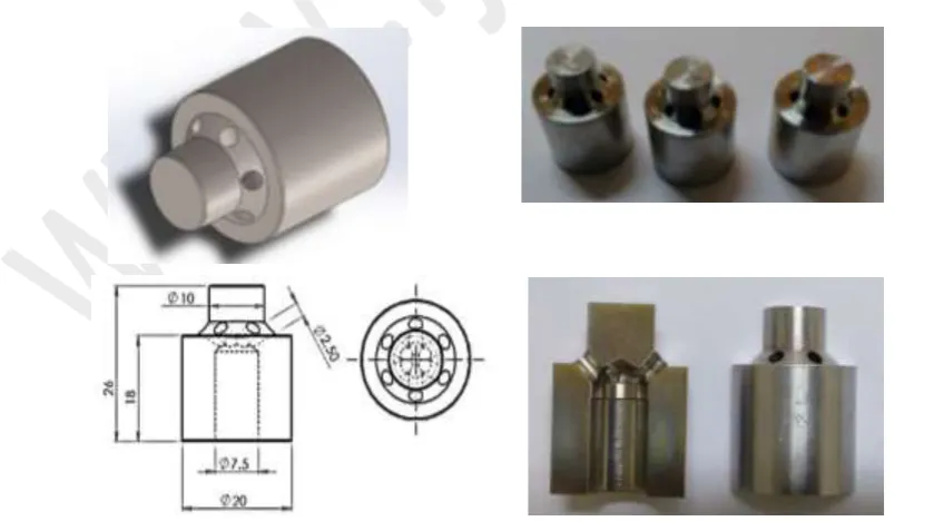
The workpiece material used in the machining test was plunger body made of stainless steel SS446. Experiment was performed in each workpiece. All workpieces were prepared in CNC machine tool with same machining condition to get same initial surface roughness value. Initial surface roughness obtained for workpieces were about 0.8 microns and nine workpieces with same initial surface roughness value were considered for experiments. All workpieces were cleaned before and after AFM with ultrasonic cleaning machine using isopropyl alcohol as cleaning agent. Plunger body shown in Figure 2.
Volume 01, No. 10, October 2015
P
age
59
ABRASIVE MEDIA SYSTEM
The abrasive media used in Abrasive Flow Machining provides the actual material removal: polishing, deburring and edge radiusing. The nine samples of media with different abrasive particle size and concentration of according design matrix were developed from VSSC Polymer lab. The abrasive media mainly consist of two parts: silicon based polymer and abrasive particles. The viscosity of silicon polymer is 700 Pa-s measured using Brookfield Viscometer. The abrasive used in this study was Silicon Carbide (SiC). Media flow rate was
560 cm3/min made constant throughout the experiments and fixture is used to guide the
abrasive media. The media is forced through the workpiece where it acts as a flexible file, or slug, moulding itself precisely to the shape of the workpiece. The pressure exerted by the fluid on all contacting surfaces also results in a very uniform finish.
Figure 3: Silicon Carbide loaded AFM media EXPERIMENTAL DETAILS
The experiments were conducted according to Taguchi method in nine workpieces. Initially the component was machined with CNC machine and the surface roughness values were measured. Later the component is machined with the developed AFM system with number of passes. The fixture is used to hold the workpiece and also guide the media through workpiece. Predetermined values of time and number of cycles were set on the timer system. After attaining all the precautions experiment was started. When experiments were completed, all workpieces were cleaned with ultrasonic cleaning machine using isopropyl alcohol as cleaning agent. After cleaning, workpieces were cut into two halves by wire cut EDM and inspected for surface roughness and edge radius. The inspection is done at the Metrology Lab, LPSC, Thiruvananthapuram. The inspection process is carried out using the Taylor/Hobson Precision Form Talysurf. The stylus probe of the Talysurf is run through a distance of 5 mm along the surface where the roughness to be measured, to obtain the Ra values. Edge radius is also obtained by running probe through inside edge of a cross drilled hole.
RESULTS AND DISCUSSIONS
Volume 01, No. 10, October 2015
P
age
60
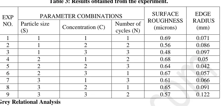
Table 3: Results obtained from the experiment.
Grey Relational Analysis
The grey relational analysis (GRA) is one of the powerful and effective soft-tool to analyse various processes having multiple performance characteristics.
Steps in GRA
1. Normalization of experimental results in GRA Normalization of Ra
Surface roughness values should be minimised to 0. So we take smaller the better equation for normalising the Ra value.
Normalization of Edge Radius
Normalization of edge radius is based on larger the better criterion because edge radius should be maximised.
where,
is the generating value of Grey relational analysis; min is the minimum
value of ; max is the maximum value of .
Finding Grey Relational Coefficient:
Grey Relational Coefficient is calculated to express the relationship between the ideal and actual normalized experimental results. The Grey Relational Coefficient can be expressed as follows:
2. Finding Grey Relational Grade: EXP
NO.
PARAMETER COMBINATIONS SURFACE
ROUGHNESS (microns)
EDGE RADIUS
(mm) Particle size
(S) Concentration (C)
Number of cycles (N)
1 1 1 1 0.69 0.071
2 1 2 2 0.56 0.086
3 1 3 3 0.48 0.097
4 2 1 2 0.68 0.05
5 2 2 3 0.64 0.042
6 2 3 1 0.67 0.057
7 3 1 3 0.61 0.066
8 3 2 1 0.65 0.091
Volume 01, No. 10, October 2015
P
age
61
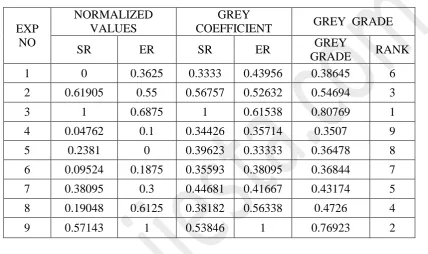
After obtaining the grey relational coefficient, the grey relational grade is obtained by taking the average of grey relational coefficients. The grey relational grade is defined as follows.
where, γi = Grey Relational Grade, n = number of response factors
Table 4: Table for calculating grey relational grade.
EXP NO
NORMALIZED VALUES
GREY
COEFFICIENT GREY GRADE
SR ER SR ER GREY
GRADE RANK
1 0 0.3625 0.3333 0.43956 0.38645 6
2 0.61905 0.55 0.56757 0.52632 0.54694 3
3 1 0.6875 1 0.61538 0.80769 1
4 0.04762 0.1 0.34426 0.35714 0.3507 9
5 0.2381 0 0.39623 0.33333 0.36478 8
6 0.09524 0.1875 0.35593 0.38095 0.36844 7
7 0.38095 0.3 0.44681 0.41667 0.43174 5
8 0.19048 0.6125 0.38182 0.56338 0.4726 4
9 0.57143 1 0.53846 1 0.76923 2
3. Find out the response table for grey relational grade :
The mean of the grey relational grade for each level of parameter and the total mean of the grey relational grade for the 9 experiments were calculated and tabulated as shown below:
Table 5: Response table for grey relational grade
PROCESS PARAMETERS
GREY RELATIONAL GRADE
LEVEL 1 LEVEL 2 LEVEL 3
MAX-MIN RANK
Abrasive Particle Size
(S) * 0.58036 0.36131 0.55786 0.21905 2
Concentration (C) 0.38963 0.46144 * 0.64846 0.25883 1
Number of Cycles (N) 0.40916 * 0.55563 0.53474 0.14646 3
Volume 01, No. 10, October 2015
P
age
62
Figure 4: Main effects for Grey relational grade
ANOVA Analysis
The purpose of analysis of variance (ANOVA) is to investigate which of the process parameters significantly affect the performance characteristics. This is accomplished by separating the total variability of the grey relational grades, which is measured by the sum of the squared deviation from the total mean of the grey relational grade into contributions by each machining parameter and the error. The analysis of variance (ANOVA) test establishes the relative significance of the individual factors and their interaction effects.
Table 7: Results of ANOVA
Source
DOF SS MS F % C
S 2 0.08712 0.04356 6.38265 35.4801
C 2 0.10712 0.05356 7.84796 43.6256
N 2 0.03765 0.01883 2.75876 15.3355
Error 2 0.01365 0.00682 1 5.55884
Total 8 0.24555
Separate multiple linear regression models are developed for both Surface roughness and edge radius. The regression model is created using MINITAB 17 statistical software package. The independent variables are the control factors and dependent variable is the response factor.
The regression equation for Surface Roughness = 0.8717 + 0.000158 S 0.00433 C 0.000622 N
The regression equation for Edge radius = 0.0139 + 0.000098 S + 0.00148 C - 0.000031 N
DEBURRING OF BURRS IN PLUNGER BODY BY AFM
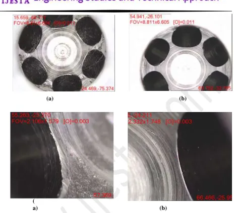
Plunger body is a precision aerospace components using in propellant control solenoid valve of LAM engine using in satellites. Micro burrs occurring inside the small cross drilled holes may result malfunctioning of flow control valve. Due to the complicated shape of plunger body manual deburring was very slow and is a difficult task. Manual deburring may lead to health and safety problems, damages the processed surface, poor repeatability and reduce
production efficiency. Figure 5 showsinner portion of plunger body before and after abrasive
Volume 01, No. 10, October 2015
P
age
63
(a) (b)
(
a) (b)
Figure 5: Inner Portion of Plunger Body (a-Before AFM, b-After AFM)
4. CONCLUSION
Volume 01, No. 10, October 2015
P
age
64
REFERENCES
i Somashekhar S. Hiremath, Vidyadhar H. M.and Makaram Singaperumal, “A Novel
Approach For Finishing Internal Complex Features Using Developed Abrasive Flow
Finishing Machine”, International Journal of Recent advances in Mechanical
Engineering (IJMECH) Vol.2, No.4, November 2013.
ii Eckart Uhlmann, Vanja Mihotovic, Andre Coenen, “Modelling the abrasive flow
machining process on advanced ceramic materials”, Institute for Machine Tools and
Factory Management (IWF), Berlin University of Technology, PTZ 1, Pascalstr. 8-9, 10587 Berlin, Germany.
iii S. Y. M. Wan, W. S. Fong, C. J. Kong, D. L. Butler and M. S. Tiew, “Low pressure
abrasive flow machining”, Volume 11, Number 1, Jan-Mar 2010, SIMTech technical
reports (STR_V11_N1_04_MTG).
iv V.K. Gorana, V.K. Jain, G.K. Lal, “Experimental investigation into cutting forces and
active grain density during abrasive flow machining”, International Journal of
Machine Tools & Manufacture 44 (2004) 201–211.
v M. Ravi Sankar & V. K. Jain, “Abrasive flow machining (AFM): An Overview”,
Indian Institute of Technology, Kanpur, 208016, India.
vi Hsinn-Jyh Tzeng, Biing-Hwa Yan,Int J, “Self-modulating abrasive medium and its
application to abrasive flow machining for finishing micro channel surfaces”, Advance Manuf TechnoL , 32: (2007) 1163–1169, Springer-Verlag London Limited.
vii RAVI GUPTA , Rahul Wandra, “Effect and optimization of Process Parameters on
surface roughness in Abrasive Flow Machining Process”, IJITKMSpecial Issue