New Algorithms for Distributed Sorting in Distributed Systems

(1)

New Algorithms for Distributed Sorting in

Distributed Systems

Muaayed F. Alrawi

Date of publication (dd/mm/yyyy): 29/06/2017

Abstract – This paper presents four algorithms to solve the distributed sorting problem in n-nodes distributed systems. Each algorithm consists of two phases. Phase (1) called "Distributed n-Selection Algorithm", which is used to find all the (𝒊 ∗ 𝑪) smallest required keys value. Phase (2) called "Records Migration Algorithm", which is used to transfer records to their appropriate nodes. Algorithm (3) has the message complexity of 𝑶(𝒏𝟑_𝒍𝒐𝒈𝑵

𝒏) in phase (1), in addition to

𝑶(𝒏) in phase (2), while algorithm 1, 2, and 4 have a message complexity 𝑶(𝒏𝟐_𝒍𝒐𝒈𝑵

𝒏) in phase (1), in addition to 𝑶(𝒏) in

phase (2) to sort a file F of cardinality N over a system of size n-nodes.

Keywords– Sorting, Distributed System, Algorithms.

I. I

NTRODUCTION

The definition of the distributed model is based on the general definitions of the distributed sorting problem presented in [1], [2], and used also by [3]. The following definition are used:

 Communication network of size n and capacity R is a set



S S1 2. ...Sn



of modes where each mode can store R records in its local nonshared memory.

 Associated with a network is a set LSXS of communication lines between nodes; If



S S_i. _j



L S and S. _i _jare said to be neighbors.

 Massage may contain only an identifier (from a predetermined alphabet), a key, a record, a counter value, positive integer or any subset of the above.

 The identities of the nodes must be distinct, otherwise no deterministic distributed algorithm is possible.

 Each node in the network contains a vector of size in to store the temporary calculation of the ranks for the system nodes in the system.

 Each node in the networks contains a matrix of size (2 ( n 1)) to store the selected Global Required Ranks value (GRRi) and the Required keys value (RKi).

 A file of cardinality N is a set F



r r1 2. ...rN



of records

r F



that contains a unique key K(r) drawn from a totally ordered set.

 A distribution of F on S is a n-tuple

   

 



2 , 2 ... n



X x S X S X S

Where X S

 

_n F is a subfile stored at node 1

 S R X S X

 

S for i j and X S F

X i

n

i j

i

i  .    . _₁  Given

a distributed X 



x S

   

₂ ,X S₂ ...X S

 

_n



of F on S, and a permutation



(1,2,………., n)



((1, 2, ………, n)), X is said to be stored according

to



if, for

i



j

rX

 

S(i)KrX

 

S(i);K(r)K(r)'i j (1) That is, the keys stored at node

S

_₍_i₎ is not greater than each key stored at node S_{ }_{( 1)}_i for 1 i n

 A node participating in a distributed algorithm behaves as a limited state machine; at each during the computation, it receives certain messages, performs some local processing and generates certain messages [2].

 Since only a subset of F is available to each node, a computation on F will in general requite both processing activities at the nodes, and communication activities between nodes. Furthermore, since local processing time is usually negligible when compared to transmission and queuing delays, the cost of any distributed computation on X is assumed to be dominated by communication coasts.

 Without loss of generality, we can assume, from the previous point that a subset of F a certain node is always sorted.

 X denotes the set of all distributions of F on S. for the purpose of calculating the expected complexity, all records of X are assumed to be similar;



n denotes the set of all permutations of the first N integers.

 A distributed algorithms is initiated at one or more nodes (usually) by a command given by the user or generated by a system operating at a node). Anode at which the algorithm is not initiated becomes active only after receiving a message from another node.

 A node can send and /or receive messages to/from all nodes. The communication links are bidirectional. This is necessary for the developed algorithm to be distributed.

The following steps are considered for any distributed algorithm:

- Each active node alternately performs local computation, if any, and sends out message to its neighbors (none, some, or all of them).

- It is assumed that a node can receive messages from is neighbors at all instances.

- Thus, no messages are lost once they are delivered to a node, not they are lost on any of the communication links (Reliable network).

- All messages are guaranteed of delivery within an arbitrary but finite amount of time (Real-time delivery).

(2)

- It is assumed that the distributed, system incorporates the necessary termination algorithms.

 Massage and time are the fundamental resources used by an algorithm. Thus, we consider the number of massage and the number of time units as the two measures of cost of a distributed algorithm. These are counted from the initiation of the algorithm to the instance when all nodes become inactive. If there is more than one possible way in which an algorithm can terminate, then the longest path in the “computation graph” of all possible executions of the algorithm is

considered.

 When a node sends copies of the same message to several of its neighbors at once, then they are considered as only one message (i. e. messages that move in parallel are counted only as one message) [1], and [3].

 To analyze the time used by a distributed algorithm, we postulate the existence of logical global clock not accessible to any of the nodes. A unit to, sends a set of messages to its neighbors, and all these messages are received within the same unit. Thus, the local delays, processing times, message queen delays, and message transmission times are all absorbed into abstraction of the unit time Clearly, the local processing times must be logical so that it does not affect the unit time.

II. P

REVIOUS

W

ORK

Few related papers have appeared in the literature recently. Most of these deal with general point-to-point networks. The general technique used is that of constricting a spanning tree first and then sorting on the tree. [4] deals the selection problems on synchronous and asynchronous networks. The researchers in [5] and [6] study the problem of finding the median of a file distributed among two nodes. In [3], the author considers two variants of the problem-static and dynamic sorting and gives optimal algorithms for large files. In [7], the researcher gives an algorithm for the sorting problem for the case of C = 1. [4] presents lower bounds and algorithms for the sorting problem on local area networks for the cases of serial and parallel connections among the nodes. In [8] derived Algorithm for Prefix Computation in Static Ad Hoc Mobile Networks with the worst case lower bound of (n − 1) rounds for distributed sorting on a line network.

III. S

PECIFIC

D

ISSERTATION

P

ROBLEM



The Distributed Sorting Problem

Distributed Sorting is defined as the problem of transferring (through communication activities) the elements of a given distribution

   

 



X S2 ,X S2 ...X Sn



among the n-nodes so that the resulting distribution



y S

   

₂ ,y S₂ ...y S

 

_n



in sorted according to some permutation



, as given in (1)



( )i





( )i



; ( ) ( ')

r X S_ Kr X S_ K r K r i j

      from

this definition, it is evident that many distribution are

possible results of sorting process at least one for n! permutation.



The Distributed Ranking Problem

Distributed ranking is the problem of assigning each node a unique number such that the number of messages required to transfer records to their final destinations is minimized.

In this dissertation proposal we explore the idea of designing a unified algorithm for sorting the records over all n-nodes without partitioning the n-nodes into smaller subsets. This new algorithms are truly distributed, in the sense that no central node has complete information about the rest of the nodes. The algorithms are topology independent.

In solving the problem of sorting in n-nodes distributed system, we'll present some algorithms, and measure the performance in terms of the number of steps required to transfer records to their appropriate nodes.

IV. D

ISTRIBUTED

S

ORTING IN N

-N

ODES

D

ISTRIBUTED

S

YSTEMS

It has been shown in this section four algorithms, each one consists of two phases. Phase (1) is used to find all (i*C)th_{smallest required keys while phase (2) is used to} transfer records to their appropriate nodes. At the end of the algorithm, a file of N records is sorted properly over a system of size n-nodes. The following terminology will be used in all algorithms presented in this section:

Tempp is the temporary variable used by each node to store the rank of a certain key value that is calculated from the previous step, mp is a key value of a record stores at rnode p, GRp (mp) is the computed Global Rank ( overall n-nodes) of a certain key value at node p, GRRi is the Global Required Ranks value i.e. the ( i*C)th_{smallest Ranks value,} LRp (mp) is the Local Rank value of a certain key value (mp) at a certain node, RKi is the Required Keys value i.e. keys value that are occupied by the GRRi (the (i*Cth) smallest key value), L and R Variables mean left and right used at each node to store ranks value that are used to select a key value, Mid is the temporary variable used to store the previous rank value, where

mp= Kp (Tempp) Mid=(L+R)/2 GRRi=(i*C) RKi=Ki (GRRi) i= 1,2, ---(n-1) p=1,2,---n

Where n is the total number of nodes in the systems, C is the total number of records stored at each nodes, N is the total number of records in file F={r1, r2,...rn} distributed over n-nodes, where each record has a unique value. It assumed that N=n*C. The four algorithms are listed below:

Algorithm (1)

Phase (1): Distributed n-Selection Algorithm: (Select All n-Nodes)

1. Procedure (1) // Get the Required-Table Begin

(3)

GRR (i):= [i*C]

Insert GRR (i) in Requited-Table End 2. Procedure (2): // Select a key-value Begin

For i:=1 to (n-1) Begin

Temp := (i*C)/n

Send m(p) (o to node (p1).

3. _{Procedure (3): // Compute the Local - Rank value} For p:=1to n

Select m(p) Begin Left :=1 Right :=C

While Left < Right Do Begin:

mid := ( Left +Right ) /2 If mid:= 1 then Return LRp (mp):= mid Else

If {(K(mid)>=m(p) and (k(mid-1)<m(p))} then Return LRp(mp):= mid

Else

If (k(mid))>m(p) then Right := mid

Else Left := mid Endif Endif Endif Endwhile

Return LRp (mp):= C+1 End.

4. Procedure (4): (Select proper-Key value) Each node after receiving mJ and mI values from node (P1), it searches For new proper key value).

Begin L:=0 R:=C

While (L = R-1) Do Begin

If mp < mJ then L:= Temp Mid:= 𝐿+𝑅₂

Selects new mp=K(mid) Else

mp > mI then R = Temp mid:= 𝐿+𝑅₂

Select new mp = K(mid) Endif

If ((mp < m(I)) and (mp > m(J))) Then Sends New selected mp

R:=C Else

send previous (old) mp R:=C

End if End.

(Select node (pI)):

5. Procedures (5): (sender a vector mp of n-keys value to (n- 1) nodes)

 Node (p1) receives all m(p) keys value

 Stores all keys value in a vector [m (1), m(2), ---, m(n)]

 sends vector (mp) to all (n- 1) nodes

 End.

6. Procedure (6): // Computes the global- ranks value

Begin

for p:= 1 to n Do Begin

GR(p). node = p

GR(p). R= sum (R(p))-n+1 End.

End.

7. Procedure (7): // Checks computed global- ranks value

Begin u:=1

While u <= n then For i := 1 to (n-1) Begin

If GR(p).R=(i*C) then return m (p) = K(GR(p). R) RK(i) := m(p)

Endif End for U:=U+1

Call-Procedure (8)

If i<(n-1) then call-procedure (2) Else terminate Phase (1).

Endif End.

8. Procedure (8): (sends mJ and mI values to all nodes)

Begin

call-sort Global - ranks procedure

If ((GR(m(J) and GR(m(I) <> 0 or (GR(m(J) <> 0 and GR(m(I) = (0) then Sends (m (J), m(I) to nodes whose key value > RK (i) If (GR (m (J) and GR (m(I) <> 0 or (GR(m(J) = 0 and GR(m(I) <> 0) then Sends (m (J), m (I) to nodes whose key Value RK(i). Endif

Endif End.

Phase (2): Records Migration Algorithm (Over all n-nodes);

- All records whose keys value ≤ RK(1); are transferred to node (1).

- RK(1) < All records,whose keys value ≤ RK(2); are transferred to node (2).

- RK(n-2) < All records whose keys value ≤ RK(n-1); are transferred to node (n-1)

- All records keys value > RK(n-1); are transferred to node (n).

At the end of this phase; the whole file F is sorted properly overall nodes and algorithm (1) is finished.

Algorithm (2)

(4)

(Select all nodes)

Procedure (1): // creating the Required - Table Begin

RKi := Ki ((GRRi) For i := 1 to (n -1) GRRi :=[i *C] End.

Procedure (2): // Selecting a key value mp Begin

i:=1 L:=0 R:=C+1

10 While i< n Do Begin

Temp:= 𝐿+𝑅₂

Select mp= Kp (Temp) Send mp=node (p1)

Wait for message from node (p1).

// Each node computes the local rank value long ifs list for each selected key value received from node (p1)

Procedure (3): // Computing the local – ranks value LRp(mp)

Begin

For P:= 1 to n Begin

Select mp Lp := 1, Rp := C While Lp < Rp Do Begin

Mid: = (Lp+Rp)/2

If (mid=1) then return LRp (mp)=1 Else

If ((Kp (mid) mp) and (Kp (mid -1)<mp) then return LRp (mp) = mid

Else

If (Kp (mid)>mp) then Rp=mid Else

Lp := mid Endif Endif Endif Endwhile

Return LRp = C+1 End.

Procedure (4): // Selecting new key value mp Begin

If (GRi (mp) equal to any GRRi) then RKi (GRRi) =mp Store mp in the Required-Table

Endif

If (Gri (mp) equal to the exact GRRi) then i:=i+1 20

If i=n then terminate phase (1) Endif

Return to the Required-Table If (next RKi is not found) then L:= Temp, R:=C

Goto 10 Else Goto 20

Endif Else

If (GRi (mp) is less then exact GRRi) then Let L:=Temp

If (L=R-1) then Let R:=C Goto 10 Else Goto 10 Endif Else

(GRi (mp) is greater than exact CRRi) then Let R:=Temp

if (L=R-1) then Let R:=C Goto 10 Else Goto I0 Endif Endif Endif End.

(Sclect node (p1))

Procedure (5): // Node (Pi) sends a copy of n-selected keys value to each node

Sends a vector m= [mp] to all nodes End.

Procedure (6): // Computing the global rank value for each selected key value Begin

For P:=1 to n Do Begin

(GR(p) node = P)

(GR(p). R=Sum (R(P)) – n + 1 Sends GR(P) to node (P) End.

End.

Phase (2): Please see phase (2) in Algorithm (1).

Algorithm (3)

Phase (1): (for each node)

Procedure (1): // Creating ills Required-Table Begin

RKi Ki ((GRRi) For i:= 1 to (n-1) GRRi:= [i*C] End.

Procedure (2): // Selecting a key value mp Begin

i:=1, L:=0, R:=C While i<n Do 10 Begin

Temp:=𝐿+𝑅₂

Select mp = Kp (Temp) Send mp to each node Wait for local rank value End.

// Each node computes the local rank value a long its list for each selected key value

(5)

Begin For p:=1 to n Begin Select mp Lp:=1, Rp:=C While Lp<Rp Do Begin

Mid:= (Lp + Rp) /2

If (mid=1) then return LRp (mp) = 1 Else

If ((Kp (mid) mp) and (Kp (mid - 1) < mp)) then return LRp (mp)= mid

Else

If (Kp (mid)> mp) then Rp=mid Else

Lp = mid Endif Endif Endif Endwhile

Return LRp (mp) = C+1 End.

Procedure (4) // Computing Global Rank value GR (mp)

Begin GR (mp) := 0 For p:=1 to n Select LRp (mp)

GR (mp)= GR (mp)+LRp(mp) Endfor

GR (mp)=GR(mp)-n+1 End.

Procedure (5): // Selecting new key value mp) Begin

If (GRi (mp) equal to any GRRi) then RKi (GRRi)= mp Store mp, in the Required-Table

Endif

If (GRi (mp) equal to exact GRRi) then 20 i:=i+1

If i=n then terminate phase (1) Endif

Return to the Required - Table

If (next RKi is not found) then L= Temp, R=C+1 Goto 10

Else Goto 20 Endif Else

If (GRi (mp) is less than exact GRRi) then L=Temp If (L=R-1) then R=C

Goto 10 Else Goto 10 Endif Else

(GRi (mp) is greater than exact GRRi) then R=Temp If (L=R-1) then R=C

Goto 10 Else Goto 10 Endif

Endif Endif End.

Algorithm (4)

(Over all nodes)

• // Each node starts with these initial values by setting

all L to 0, all R to (C + 1) and active to true for i:= l to (n-1) Do

Begin

L[i]:=0, R[i]:=C+1, Active[i]:=true End.

 //Each node compute Local-Rank LRp (mp) For i:=1 to (n-1) Do

Begin

Setects (m[i]); For j:= I to C Do If m [i]<K[j] then

Let LRp (m[i]) := (j-1), L[i]:=(j-1) Sends LRp (m[i]) to the leader node End.

(Ovcr a leader node)

 // Selects key (s) value m[i] While active [i]:= true Do Begin

For i:= 1 to (n- 1) Do Begin

If active [i] Begin

Temp[i]:= (L[i]+R[i])/2 m [i]:=k (Temp [i]) End.

End.

 //Sends all m[i] to all (n-1) nodes For i:=1 to (n-1) Do

If active[i] Do Begin

For j:=1 to (n-1) Do sends to each node (i, m[i]) waits for Local Ranks LRp (mi). End.

 //After receiving all Local – Ranks LRp (mi), computes Global- Ranks GRi (mi)

For i:=1 to (n-1) Do If active [i] then Begin

GRi (mi):=Temp [i]; For j:=1 to (n-1) Do

GRi (mi):= GRi (mi) +LRp (mi) [j] End.

 // Checks all Global-Ranks, selects new key (s) value and sends to each node //

i:=1 to (n-1) Do For If active [i] then

Begin

1f GRi (mi) =i*C then Beign

Let Rk [i]:= m [i] active [i]: = False End.

(6)

If GRi (mi) > i*C then R[i]:=Temp [i]; Else

L[i]:=Temp [i]; If L[i]:=(R[i]-1) then active [i]:= False Else

Temp [i]= (L[i]+R[i])/2 selects m[i]=k(Temp[i])

sends all m[i] to each node in the system. End.

End. End while

 // Previous leader node sends messages to the next node to be a leader node

For i:=1 to (n-1) Do

If (RK[i] is not found and L[i]= R[i] - 1) then sends keys value (k(R[i]), k([i])) to next leader node Exit

(Over next leader node)

 // The starting work of the next leader node after receiving K(R[i]) and K(L,[i])

For i:=1 to (n-1) Do

If (K (R [i]), K([i])) are received) then Begin

L[i]:=Local Rank (K(L[i])) R[i]:=Local Rank (k(R[i]) + 1) End.

 //Continues as a leader node//.

Phase (2): please see other algorithms

IV. S

IMULATION

A

NALYSIS

The algorithms presented in section III are simulated using C++ language programs. Each program is used to calculate practical (average) number of' messages to selected all required keys over n-nodes as follows. It distributes a list of numbers among certain number of nodes at random and then finds all required keys. It calculates the number of iterations, the number of time steps and the number of messages that are required to find all required keys.

The program is repeated for many times for the same number of nodes and records to calculate the average.

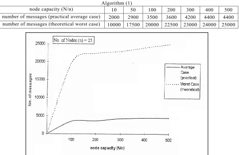
Figures (1, 2, 3, 4) show the average number of messages required to select all required keys among 25-nodes with different node capacity (N/n) compared to those computed theoretically for the worst case for algorithms 1,2,3 and 4 respectively.

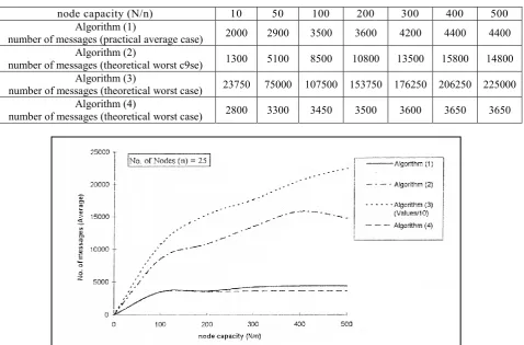
Figures (5) shows a comparison between the average number of messages required to select all required keys obtained from all algorithms (1,2,3 and 4) for fixed number of nodes (n=25) and different node capacity (N/n).

Simulation Results:

1- Total number of nodes (n) = 25

Algorithm (1)

node capacity (N/n) ₁₀ ₅₀ ₁₀₀ ₂₀₀ ₃₀₀ ₄₀₀ ₅₀₀

number of messages (practical average case) 2000 2900 3500 3600 4200 4400 4400 number of messages (theoretical worst case) 10000 17500 20000 22500 23000 24000 25000

(7)

Algorithm (2)

node capacity (N/n) 10 50 100 200 300 400 500

Fig. (2): Comparison between the average and the theoretical worst case number of messages for different node capacity (N/n), algorithm (2).

Algorithm (3)

node capacity (N/n) 10 50 100 200 300 400 500

(8)

Algorithm (4)

node capacity (N/n) 10 50 100 200 300 400 500

Figure (4): Comparison between the average and the theoretical worst case number of messages for different node capacity (N/n), algorithm (4).

node capacity (N/n) 10 50 100 200 300 400 500

Algorithm (1)

number of messages (practical average case) 2000 2900 3500 3600 4200 4400 4400 Algorithm (2)

number of messages (theoretical worst c9se) 1300 5100 8500 10800 13500 15800 14800 Algorithm (3)

number of messages (theoretical worst case) 23750 75000 107500 153750 176250 206250 225000 Algorithm (4)

number of messages (theoretical worst case) 2800 3300 3450 3500 3600 3650 3650

Figure (5): Comparison between the average (practical) numbers of messages for different node capacity (N/n), for all algorithms.

V. C

ONCLUSION

Four distributed sorting algorithms in n-nodes distributed systems are presented in this paper: Each algorithm is divided into two phases. Phase (1), is used to find all the (i*C)th _{smallest required keys} value while phase (2) is used to transfer records to

(9)

value to a node leader. In algorithm (1), the number of iterations required to final all (i * C)th_{required keys} the worst case is (𝑛 (1 + log𝑁_𝑛)), and the total messages exchanged in phase (1) in the worst case is

(4𝑛2_{(1 + log}𝑁

𝑛)). The total messages exchanged in

phase (2) is (2(n-1)).

Therefore; algorithm (1) has a message complexity of

O (𝑛 (log𝑁_𝑛)).

Since most of; the work done by only one node (say, node (p1), thus the number of time Steps and the computation time per iteration is larger than those ill others algorithms. In algorithm (2):

- Each node starts with the selection of- its median key value along its list, then continue searching for all required keys value by using the binary search principle, i.e., continues moving through its list without returning back to any previous position.

- When a node does not find a required key value, it does not wait until another node finds such required key. instead, it goes to searching for the next required key value.

Still in this algorithm the system depends on one node to do most of the work, which means larger time steps and high compilation time taken by this leader node to compute all global ranks, but less than those of algorithm (1).

Algorithm (2) has a message complexity in worst case equal to O (𝑛 (log𝑁_𝑛)).

In algorithm (3), we have tried to distributed the works equally over all nodes. Therefore, each node in the system sends keys selected from its list to all nodes, computes local ranks value for other selected keys received from others nodes, computes and checks global rank value of its key value.

In this algorithm, since each node does part of tale work, therefore: this algorithm has less number of time steps and less computation time compared to those of algorithm (2). But algorithm (3) has message complexity equal O (𝑛3_(log𝑁

𝑛)) to which is worst

compared to the one of algorithm (2). In algorithm (4); we let only one node called the leader node to do the following operators:

- Sends messages to all nodes.

- Computes local and global ranks value.

All others nodes search with the leader node for the required keys without sending a single key value from their list, and the only work they do is calculating the local ranks value for the incoming keys value from the leader node.

Due to the above mechanism used in algorithm (4), this algorithm has the following advantages overall other algorithm described in this paper.

- It has goad message complexity which is of the order O (𝑛2_(log𝑁

𝑛)) .

- It shared algorithm (3) in reasonable computation time to do the local and global rank computation. - It has the lowest number of time steps.

- It has the lowest number of keys value exchanged with messages between all nodes

.

R

EFERENCES

[1] UDI Manber, “Introduction to algorithms”, A Creative Approach,

Addison-Wesley, 2004.

[2] K. V. S. Ramarao, “Distributed sorting on local Area Network”,

IEE Transactions on computers, Vol. 17. No. 2- February1988. [3] D. Rotem, N. Santoro, J. R. Sidney, “Distributed Sorting “, IEE

Transaction on computers, Vol. C-34 No. 4 April 1985. [4] G. N. Frederickson, “Tradeoffs for Selection in distributed

Networks” Proc. 2nd_{ACM Symp Princ. Distrib. Comput. Aug,}

1983, PP. 154-160.

[5] F. Chin and H. F. Ting, “A near-optimal algorithms for finding

median distributively”, in Proc. 5th_{Int. Conf. Distributed Compute}

System May 1985, PP. 459-465.

[6] M. Rodeh, “Finding the median distributively”, LCSS. PP. 162-166, 1982.

[7] S. Zaks, “Optimal distributed algorithms for storing and ranking

“. IEEE Trans Compute, Vol. C-34, PP. 376-379, April 1985.

[8] R. Rajendra Prasath, “An alternative time - optimal distributed

sorting algorithm on a line network”, IEEE 6th International

Conference on Network computing, Vol. 16757, PP.1-6, 2010.

A

UTHOR

’

S

P

ROFILE