ISSN: 2374-2348 (Print), 2374-2356 (Online) Copyright © The Author(s).All Rights Reserved. Published by American Research Institute for Policy Development DOI: 10.15640/arms.v4n1a7 URL: https://doi.org/10.15640/arms.v4n1a7
Bayesian Tobit Principal Component Regression with Application
Fadel Hamid Hadi Alhusseini
1Abstract
Tobit is considered an important statistical modeling, as it has become common in numerous practical applications, such as econometrics, biological sciences, finance, and medicine. The Tobit regression model is special case of censored regression model at zero point. In some cases, Tobit regression model is exposed to econometrics problems, including the multicollinearity problem. Most of the independent variables from economic, social, and medical field are overlapping with each other, thus, estimating the parameters of the Tobit model may lead to are biased and inconsistent estimation. In order to overcome this issue, a set of methods can be deployed, such as principal component. In this paper, the Bayesian technique will be used for estimating the parameters of the model. The case study included in the paper is the medical problem of the abortion within Iraqi women. The estimation was performed by using Bayesian Tobit principal component regression model through building algorithm in programing language (R).
Keywords: Bayesian Technique, Principal Component Regression, Tobit Model, Abortion.
1. Introduction
Spontaneous abortion or miscarriage is a natural method of expulsion of the fetus from the utero, in case there are detected abnormalities, like diseases or fetus death. Spontaneous abortion occurs for 15% to 20% of all cases of pregnancy and often the pregnancies are lost in the first three months of gestation. There is a set of biological, social, and economic variables that can affect the spontaneous abortion. The phenomenon under study contains one response variable that has two parts: the number of abortions that equal zero (censored part) and the number of abortion that equal one or are higher than one (uncensored part). The Tobit model is based on data of the phenomena under study. The censored part takes cumulative distribution function (c.d.f) for normal distribution and the uncensored part takes probability density function (p.d.f) for normal distribution.
As a result, the Tobit model is mixture between (c.d.f) and (p.d.f) for normal distribution. In this study, the response variable is affected by a set of independent variables. After testing the model, the results show that the model suffers from multicollinearity problem, according to Farrar-Glauber test. In order to overcome this issue, the principal components method will be used by transforming the original linked variables into unlinked new variables, representing the principal components. Each principal component will contain original variables. For estimating the parameters for Tobit principal components regression model, the Bayesian technique will be employed, after filtering the model from multicollinearity problem, through using principal components method. This parameter will be used for estimating the original coefficients for Tobit model through building algorithm in programing (R).
The rest of this paper is organized as follows: Section 2 includes a study of the Tobit regression model, Section 3 illustrates the methodology of principal component regression, Section 4 includes the Bayesian Tobit principal components regression, Section 5 details the estimation of original parameters, Section 6 shows a sample of the case study, Section 7 includes the analysis of the case study results and Section 8 highlights the conclusions. 2. Tobit regression model
The Tobit model was proposed in the middle of the last century by researcher James Tobin (1958). The Tobit model considers special a case of censored regression model, where the censored point is equal to zero (a=0). The censored regression model general formula is as follows:
=
∗≤
∗ ∗> 1)
ℎ ∗= + , = 1, … … . ,
where is an ( × 1) vector of latent variable, is a 1 × vector of explanatory variables, is a ( × 1) vector of regression parameters and is an ( × 1) vector of random error, where ~ (0, ).
If (a=0), the censored regression model will become Tobit regression model as follows:
= 0
∗ ≤0
∗ ∗> 0 2)
ℎ ∗= + , = 1, … … . , .
Whereas, latent variable distributes normal distribution for mean ( )and variance ( ), then the probability density function of takes the formula as follows, if ( = ∗) ( ∗> 0):
( ∗) = 1
√2
∗−
2 3)
The probability density function in (3) belongs to continuous part (uncensored part). Equation (3) can be rewritten as follows:
( ) =1
∗−( )
4)
and the censored part will take (c.d.f) for normal distribution as follows, if
( = 0) ( ≤0)⟶ Φ −( ) =Φ 0−( ) = Φ −( ) = 1− Φ ( )
5)
( ) = 1
∗−( )
1− Φ 6)
The function of the Tobit model in (6) is mixed between censored and uncensored parts (see William H. Greene, 2007). For estimating parameters of Tobit regression model may be depended on maximum likelihood or (O.L.S), through numerical method. Estimating parameters of Tobit model has become a routine operation because of the numerous available packages. Nevertheless, in this paper, the Tobit model suffers from multicollinearity problem. Therefore, the issue must be solved before estimating its parameters.
3. tobit principal component regression method
Each regression models is exposed to a set of econometrics problems. One of these problems is the multicollinearity problem. This problem appears when the independent variables are linked linearly or when the independent variables have perfect relationship. This perfect relationship leads to violation of the rank condition (rank(X)<p, where p is the number of independent variables). In this case, we cannot find the inverse information matrix ( ). Therefore, we cannot estimate the parameters model. In some case, the determinant of the information matrix can be relative for zero (|X X|≈0). In this case, the parameters model can be estimated, but these estimations will be inaccurate, as the variance of the parameters will be very large. Therefore, test (t) gives fake information about the independent variables confidence. A reasonable method to overcome this problem must be identified. For solving the multicollinearity problem, various sets of methods are available. Each method has properties and characteristics. In this paper, we will use the principal components method in the treatment of the multicollinearity problem in Tobit model. The principal components are orthogonal linearity compotation from independent variables (X) as follows:
= Γ
7)
where is the matrix of principal components from rank ( ∗ ) , Γ is the orthogonal matrix from eigenvector corresponding to eigenvalue in the information matrix ( ) with rank ( ∗ ), elementsγ = 1, … … . . and column Γ(j=1,2,…..q). This matrix makes from information matrix ( ) orthogonal matrix under the assume eigenvalue for matrix( ). For ≥ ≥ ⋯ ≥ the composition Tobit regression model in equation (3) on principal components where the latent variable as function of orthogonal principal component instead of original independent variables (X):
( = Γ) ∗ Γ
Γ = ΓΓ where ΓΓ = Γ Γ= I 8)
= Γ 9)
After compensation of the equation (10) in equation (3) the Tobit principal components regression model will be as follows:
= 0
∗≤0
∗ ∗> 0 10)
Where = Γ + ,
= 0
∗≤0
∗ ∗> 0 11)
∗ = θ+
The known Tobit model is a mixture model between uncensored observation ( = 0, if ∗≤0) and the censored observation ( = ∗ ∗> 0). Therefore, the Tobit principal components regression model takes the following form:
( ) = 1
∗−( θ)
1− Φ ( θ) 12)
= 1
∗−( θ)
1− Φ ( θ) 13)
We can use the maximum likelihood method for estimating the parameters of the Tobit principal component regression. In this paper, the Bayesian technique for estimating parameters of Tobit principal components regression will be used.
4. Bayesian Tobit principal components regression
The Bayesian technique is considered an advanced method in estimating parameters of the Tobit principal components regression. It has a set of features, such as Bayesian technique that is able to estimate parameters even if the sample size is small (see Alhamzawi, R., K. Yu, and Benoit, D. F, 2012). The Bayesian technique also updates the parameters through prior distribution. From the equation (13),the Tobit principal component regression is the following:
= 0
∗ ≤0
∗ ∗ > 0 ∗=θ + ,
where Y is the response variable, ∗ is the latent variable, is principal components, is the random error term distributed according to normal distribution with mean (zero) and variance ( ), therefore the Bayesian hierarchicalmodel given by:
= 0
∗ ≤0
∗ ∗> 0
where ⇒ = ( ∗, 0)anthor formula for Tobit model
∗| , , ~ ( θ, )
The probability density function for latent variable is:
( ∗| , , ) = 1
√2
∗
The joint distribution of ∗= ( ∗, … , ∗) = ( , … , ) , = (θ , … .θ ) is the following:
( ∗| , , ) = 1
√2
∗
15)
( ∗| , , ) = ( 1
√2 )
∑ ∗
16)
For finding the estimation of parameters( , ) prior distribution will be used. According to Claiming yu and Mooyd (2011), the researchers can use any prior distribution for parameters, but selecting suitable prior distribution leads to good results for posterior distribution.
4.1 Prior Distribution Specification
The coefficients of the regression model have a range from(−∞,∞). Therefore, the prior of coefficient regression takes normal distribution. By assigning zero, the normal prior distribution for θ takes the following form:
(θ| ) = 1
√2 −
θ
2 , 17)
The parameter has range (0,∞). Inverse gamma can be used for parameter , with prior taking the form of:
( | , ) =
Γ( )( ) , 18)
Where a, b are hyper parameters. 4.2 Posterior Computation Inferences
In order to obtain the posterior distribution of the coefficient regression model, multiple joint functions will be used in equation (16) by the prior distributions in equations (17) and (18), as follows:
(θ, | ∗, ) = ( ∗| , , ) * (θ| )∗ ( | , )
(θ, |, ∗, ) = ( 1
√2 )
∑
∗ 1
√2 −
θ
2 ∗Γ( )( )
19) Posterior distribution for parameterθ:
(θ, | ∗, ) = 1
√2
∑ ∗
∗ 1
√2 −
θ 2
The posterior distribution θ is distributed according to the distribution of normal with
Posterior distribution for parameter :
( |θ, ∗, ) = ( 1 √2 )
∑ ∗
∗ 1
√2 −
θ
2 (20)∗Γ( )( )
The posterior distribution of parameter is distributed according to inverse gamma distribution with Shape parameter + and scale parameter(∑
∗−
2− θ 2− ). Tobit principal components regression model can be estimated through buildingGibbs samplers that are derived for all posteriordistributions, after taking the mean for thousands iterations for all posterior distributions.
5. Estimation of original parameters
We can find the coefficients of the original variables ( ), through using the relationship between coefficients and the coefficients of the principal componentsθ:
Γ =θ ΓΓ = 1 ΓΓ =Γθ
=Γθ 21)
The coefficients are distributed according to the normal distribution by mean(Γθ)and variance ∑ . Then, ~ (Γθ , ∑ ).Also, the variance of parameter depends on the Eigen value for the information matrix( ). Therefore, the variance of parameter will be affected by a small Eigen values. Which leads to inflated parameters variance.
The principal component is become overlapping with various fields form statistics such as, it is overlap with fuzzy technique (seeGeorgescu, V (1996)). Also the principal component used to overcome on multicollinearity problem, the small Eigen values will be canceled corresponding to last principal components in the informationmatrix( ).For reducing the total variance of the parameters, the study will focus on principal components corresponding to large Eigen values.
There is a set of criteria for excluding non-dominant principal components for analysis. The principal components with eigenvalues less than (1)will exclude from analysis, were considered (see Jeffers (1967), Chatterje and price (1991)). In the same topic, Morrison (1976), mentions that depending on principal components, 75% of the total variance can be explained. For building a Tobit regression model on dominant principal components and exclude non-dominant principal components, the number of principal components is (q), thither dominant principal components are r and non-dominant principal components is (q-r). Therefore, (q-r) is excluded from the analysis, using only r as principal components. By existence of the orthogonal feature, the values of the estimated parameters
(θ) are not different, whether using all the principal components or part of them.
θ =Λ 22)
The parameter vector θ will result through partitioning the matrixΓ= Γ,Γ where: Γ = [Γ,Γ , … …Γ ], Γ = , , ,…… .
In this case, the principal component may be reduced as follows: = , . Therefore, the principal components in the analysis are: = [ , , … … . , ]andθ = θ ,θ .
After calculating the results on estimators for the parametersθ , they will be used for estimating the original parameter of the Tobit model, as follows:
= Γ θ 23)
The estimation of the original parameter for Tobit model will result from the parameters dominant principal components:
= θ , = 1,2,3, … . 24)
Through the equation (22) the Tobit regression model parameter can be estimated after building the algorithm in programming language {R}.
6. Sample of the case study
Data for the current study was collected from the Al-Shamia hospital in Iraq with the sample size consisting of 300 observations. The sample of study has one response variable, which is the number of spontaneous abortions at women. Some of the respondents have had several abortions, while some of them reported none. The response variable of this study is censored at zero point. The censored observations number is (215), by percentage - (64%). The uncensored observations number is (85), by percentage - (36%). This study contains 10 independent variables described below:
- Mother’s age: abortion number may be influenced by the age of the mother; from medical point of view, there are biological changes in the mother’s womb when the mother is above 18 years of age
- Mother’s weight: the high or low weight of the mother may influence the occurrence of spontaneous abortion
– Mother’s blood pressure: the elevated or low blood pressure of the mother may influence the occurrence of spontaneous abortion
– mother’s blood sugar:the blood sugar levels of the mother may influence the occurrence of spontaneous abortion; from medical point of view, the mother certain blood sugar levels cause increased weight of the fetus
- Number of births: frequent births may influence the occurrence of spontaneous abortion
- Working hours of the mother: there is a negative relationship between the number of working hours of the mother and the occurrence of spontaneous abortion
– Progesterone: low levels of progesterone hormone of the mother may influence the occurrence of spontaneous abortion
− Misuse of medicine: may cause problems for the fetus and this lead to spontaneous abortion
– Toxoplasmosis is considered one of the most common diseases in Iraq, and in some cases this disease causes spontaneous abortion.
After collecting all data, the algorithm for the data analysis was built using {R}. 7. Analysis of study Results
The independent variables suffer from multicollinearity problem, as can be seen in Table no. 1. Table no. 1 - Test of Farrar-Glauber
= 12543.213 = 122.34
From Table no. 1, x is greater than x ,therefore, the conclusion is that the model suffers from multicollinearity problem and the parameters of Tobit regression model cannot be estimated due to this issue, as the estimation will be abnormal. In order to overcome this issue, the principal component method will be used.
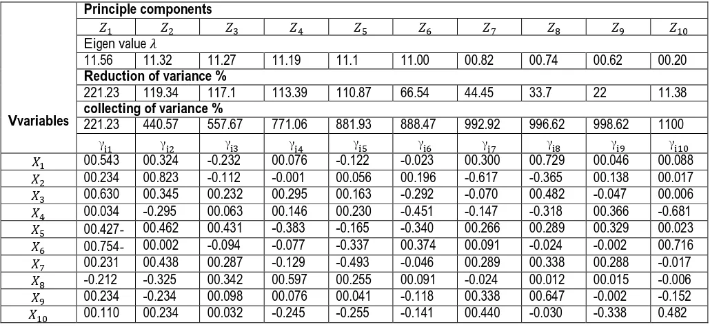
Table no. 2 - Eigen Values and Eigen Vector for Principal Component
Vvariables
Principle components
Eigen value
11.56 11.32 11.27 11.19 11.1 11.00 00.82 00.74 00.62 00.20
Reduction of variance %
221.23 119.34 117.1 113.39 110.87 66.54 44.45 33.7 22 11.38
collecting of variance %
221.23 440.57 557.67 771.06 881.93 888.47 992.92 996.62 998.62 1100
γ γ γ γ γ γ γ γ γ γ
00.543 00.324 -0.232 00.076 -0.122 -0.023 00.300 00.729 00.046 00.088
00.234 00.823 -0.112 -0.001 00.056 00.196 -0.617 -0.365 00.138 00.017
00.630 00.345 00.232 00.295 00.163 -0.292 -0.070 00.482 -0.047 00.006
00.034 -0.295 00.063 00.146 00.230 -0.451 -0.147 -0.318 00.366 -0.681
00.427 - 00.462 00.431 -0.383 -0.165 -0.340 00.266 00.289 00.329 00.023
00.754 - 00.002 -0.094 -0.077 -0.337 00.374 00.091 -0.024 -0.002 00.716
00.231 00.438 00.287 -0.129 -0.493 -0.046 00.289 00.338 00.288 -0.017
-0.212 -0.325 00.342 00.597 00.255 00.091 -0.024 00.012 00.015 -0.006
00.234 -0.234 00.098 00.076 00.041 -0.118 00.338 00.647 -0.002 -0.152
00.110 00.234 00.032 -0.245 -0.255 -0.141 00.440 -0.030 -0.338 0.482
Excluding on-dominant principal components has no effect on building the principal components regression for Tobit model because any principal component contains all independent variables. As a first step, the response variable (Number of abortions per woman) was composed on dominant principal components as shown in following table.
Table no. 3: Regression Model for Number of Abortions per Woman on dominant Principal Components
p-value t-value Regression coefficient Principal component 0.020 10.34 0.040 Intercept 0.023 -3.74 -0.124 0.040 10.78 0.164 0.000 13.90 0.207 0.000 -16.30 -0.066 0.000 5.04 0.032 0.000 2.432 0.453
By using estimators of regression model (Number of abortions per woman) on dominant principal components, the regression model will have the following results.
Table no. 4 -Tobit Principal Component Regression Results Coefficients of Regression (Number of abortions per woman) on Original Variables
p-value t-value Regression coefficients Variables 0.000 -0.325 -0.0263 Intercept 0.023 -7.435 -0.0003 0.083 4.216 0.0197 0.000 36.187 0.0170 0.567 3.345 0.0512 0.756 -0.180 -0.1061 0.004 0.132
0.008 -
0.034 4.436 0.2147 0.045 11.435 0.0618 0.000 2.934 0.5012 0.000 2.122 0.1024
Table no. 4 shows that the independent variables either positive relationship, either inverse relationship, as follows:
(Mother’s age) is significant from statistical point of view; this variable is in inverse relationship with the number of abortions –if the variable (mother’s age) increases, the number of abortion decreases
(Mother’s weight) is not significant from statistical point of view; this variable is in positive relationship with the number of abortions: if the variable (mother’s weight) increases over the limit, the probability of spontaneous abortion occurrence increases
(Mother’s blood sugar) is non-significant from statistical point of view. (Number of births) is not significant from statistical point of view.
(Monthly income of the family) is significant from statistical point of view; this variable (monthly income of the family) is in inverse relationship with the number of abortions – if the monthly income of the family increases, the number of the abortions decreases.
(Working hours of the mother) is significant from statistical point of view; t in the variable (working hours of the mother) is in positive relationship with the number of abortions.
(Progesterone) is significant from statistical point of view; the variable (progesterone) is in inverse relationship with the number of abortions – if the level of progesterone decreases, the number of abortions increases.
(Misuse of medicine) is significant from statistical point of view; the variable (misuse of medicine) is in positive relationship with the number of abortions – if the variable decreases, the number of abortions decreases. 8. Conclusion
The model under study suffers from multicollinearity problem, whichis obvious in the Farrar-Glauber test , as shown in the Table no.1.
= 14.11 ,
Where the value of (∑ ) is greater than the number of independent variables( = 10), meaning that the model has multicollinearity problem.
The number of dominant principal components is six out of ten. The dominant principal components can explain 88.47% of the total variance, meaning that the dominant principals component have explanatory power.
According to the phenomena under study, the significant variables on the number of abortions are the following:
(Mother’s age) – is in inverse relationship with the number of abortions.
(Mother’s blood pressure) – is in positive relationship with the number of abortions. (Monthly income of the family) – is in inverse relationship with the number of abortions. (Working hours of the mother) – is in positive relationship with the number of abortions. (Misuse of medicine) - is in positive relationship with the number of abortions.
References
Alhamzawi, R., K. Yu, and D. F. Benoit (2012). Bayesian adaptive Lasso quantile regression.Statistical Modelling 12, 279–297. 5, 16.
Intrilligator, M. D.,(1996)" Econometrics Models”, Techniques and Applications", Prentice Hall.
Farrar, D. E. and Glauber, R. R. (1967) Multicollinearity in regression analysis: the problem revisited, Review ofEconomics and Statistics, 49, 92-107.
Georgescu, V (1996). A fuzzy generalization of principal components analysis and hierarchical clustering. In Proceedings of the Third Congress of SIGEF, Paper 2.25. Buenos, Aires.
JEFFERSJ., N. R. (1967).Two case studies in the application of principal component analysis. Appl. Statist., 16, 225-236.
Tobin, James (1958)"Estimation of Relationships for limited dependent Variables " Econometrica, January 26, pp24-36 .
Yan, Xin, Gang Su, Xiao, 2009: "Linear Regression Analysis, Theory and Computing". puplished by world scientific puplishing. Co. Pte. Ltd, London.
Yu, K. and R. A. Moyeed (2001). Bayesian quantile regression. Statistics &ProbabilityLetters 54, 437–447. 4, 6. Reference to a chapter in an edited book:
Morrison (1976)MULTIVARIATE. STATISTICAL METHODS. The Wharton School. University of Pennsylvania. McGraw-Hill, Inc. New York St.
Chatterjee, S. and Price, B. (1991), “Regression Diagnostics”, New York: John Wiley.