Vol. 5, No. 2, 2013 Article ID IJIM-00290, 11 pages Research Article
Characterizing and finding full dimensional efficient facets of PPS
with constant returns to scale technology
G. R. Jahanshahloo ∗, I. Roshdi †‡, M. Davtalab-Olyaie §
————————————————————————————————–
Abstract
In DEA (Data Envelopment Analysis), the Full Dimensional Efficient Facets (FDEFs) of PPS (Pro-duction Possibility Set) play a significant role and have many useful applications. In this research, we, first, provide a detailed characterization of the structure of FDEFs of the PPS with constant returns to scale technology, using basic concepts of the polyhedral sets theory. Then, using the mentioned characterization together with a mixed integer linear programming, we propose an effective algorithm for finding all of the FDEFs of the PPS. We will elaborate on our algorithm by an illustrative example.
Keywords: Data envelopment analysis; Production possibility set; Weights and multipliers; Full di-mensional efficient facet; Polyhedral set; Mixed integer linear programming.
—————————————————————————————————–
1
Introduction
D
EA is a mathematical programming methodfor evaluating the relative efficiency of Deci-sion Making Units (DMUs) with multiple inputs and outputs. The relative comparison in DEA is performed within a production possibility set (PPS), which is empirically constructed from the observations by assuming several postulates (see [16]) and DEA forms an empirical frontier. The efficient frontier is the main part of the PPS’s frontier. The FDEFs of the PPS form the effi-cient frontier, which play a significant role and have many useful applications in DEA, e.g.,
1. Uniquely identifying a reference set for a given DMU that contains the maximum
∗Department of Mathematics, Science and Research
Branch, Islamic Azad University, Tehran, Iran.
†Corresponding author. [email protected]
‡Department of Mathematics, Science and Research
Branch, Islamic Azad University, Tehran, Iran.
§Faculty of Mathematical Science and Computer
Engi-neering, Tarbiat Moallem University, Tehran, Iran.
number of efficient DMUs. In this way, if we consider the efficient projection of the given DMU, we can simply determine the set of all FDEFs on which this efficient projection is lying. Consequently, the reference set of DMU will be the set of the efficient DMUs that are lying on the intersection of these FDEFs.
2. Sensitive and stability analysis in DEA [8].
3. Finding the closest target for a given ineffi-cient DMU. For this purpose as mentioned in [10,12], one can simply measure the mini-mum distance between given DMU from each of the FDEFs, and at last determine the min-imum value of these distances.
So far, about finding FDEFs and their struc-ture, several papers have been written while none of them has directly and comprehensively dis-cussed about them. Yu et al. [9] studied the structural properties of DEA efficient surfaces of the PPS under the generalized DEA model. Olsen and Petersen [14, 15] provided an outline
of possible uses of complete information on the facial structure of PPS. Also they proposed two algorithms based on the set so-called Ejo. They
stated that: “The only candidates for spanning an FDEF including any given DMUjo; jo ∈ E,
are those that can be termed efficient along with DMUjoitself. Let Ejodenote an index set for this
set of extreme efficient DMUs.” Here, the ques-tion is that how it is possible to determine Ejo
without having all of FDEFs on which DMUjo
is lying. In fact, to determine the Ejo we need
all FDEFs on which DMU is lying. Therefore, the foundation of their algorithms has this serious problem and for implementing their algorithms, a method is required to determine Ejo without
having FDEFs. Recently, Jahanshahloo et al. [6] proposed an algorithm for finding the “strong defining hyperplanes” of PPS. They proved that in evaluating an extreme CCR-efficient DMU the hyperplanes that are corresponding to the ex-treme optimal and strictly positive solutions of the multiplier form of the CCR model, are strong defining hyperplanes. Their approach has several computational difficulties that are summarized as follows:
1. They perform the algorithm for all CCR-efficient (extreme and non-extreme) DMUs, while the number of these DMUs may be a large one.
2. To employ their proposed algorithm, the multiplier form should be solved via the sim-plex method. Moreover, all the extreme (basic feasible) optimal solutions should be found, while there does not exist an effective method for performing this task. Further-more, none of these solutions is necessarily strictly positive and the algorithm may be yielded some extreme (basic feasible) opti-mal solutions that have the zero components.
3. Through implementation of the algorithm for different DMUs, many iterated strong defining hyperplanes may be generated where their algorithm is unable to prevent this.
In this paper, first, using basic concepts of the polyhedral sets theory, we seek to provide a de-tailed characterization of the structure of FDEFs, and secondly, we propose an effective algorithm
for finding all FDEFs of PPS. As we will demon-strate in Section 4, our algorithm is computa-tionally better than those algorithms mentioned above.
The paper unfolds as follows: The primal and dual descriptions of the PPS with focus on the representation of the constant returns to scale technology are reported in Section 2. An applied model for identifying the extreme-efficient DMUs is presented in this section, as well. Section3 in-cludes the characteristics and structure of FDEFs of PPS. In Section 4, we will develop the new method for finding all of the FDEFs. An illustra-tive example is documented in Section 5, which intuitively describes the new algorithm. The con-clusion and future directions for research are sum-marized in the last section.
2
Background
Consider n observed DMUs, DMUj, j =
1, 2, ..., n, which use the same number, m, of in-puts, xij, i = 1, 2, ..., m, to produce the same
number, s, of outputs, yrj, r = 1, 2, ..., s. The
input and output vectors of DMUj respectively
are denoted by xj and yj; we assume that they
are nonnegative and neither one is equal to zero. We use (xj, yj) to describe DMUj, and consider
DMUo as the DMU under evaluation. Further,
as stated in [2], “We say that a data domain is in reduced form if for no pair (j, k) withj ̸=k and the scalar α is DM Uj = αDM Uk.” We assume
that the data domain is in reduced form.
Under the standard assumptions ofInclusion of observations,convexity,constant returns to scale
and free disposability of inputs and outputs, the unique non-empty PPS is generated from a set of n observed DMUs, DMUj, (j= 1, 2, ..., n), is as
follows:
Tc={(x, y)∈R≥m0+sx≥ n
∑
j=1
λjxj ,
y≤
n
∑
j=1
λjyj, λj ≥0, j= 1,2, ..., n}.
Charnes et al. [1], relative to Tc, introduced
of DMUo:
M in θ
s.t. ∑∑nj=1λjxj ≤θxo, n
j=1λjyj ≥yo,
λj ≥0, j= 1,2, ..., n.
(2.1)
This program is called the envelopment form (input-oriented) of the CCR model. DMUo is
ra-dial efficient if θ∗ = 1; And is CCR-efficient if and only if it is radial efficient and all constraints (except the nonnegative ones) are binding at all optimal solutions. In other words, DMUois
CCR-efficient if and only if it is radial CCR-efficient and the optimal value of model (2.2) (called Additive model) is equal to zero:
M ax ∑mi=1s−i +∑sr=1s+r
s.t. ∑∑nj=1λjxij +si−=xio, i= 1,2, ..., m, n
j=1λjyrj −sr+=yro, r= 1,2, ..., s,
λj ≥0 , s−i ≥0, s+r ≥0 ,
j= 1,2, ..., n , i= 1,2, ..., m , r= 1,2, ..., s.
(2.2) The dual form of model (2.1) is called the mul-tiplier form of the CCR model and is as follows:
M ax Utyo
s.t. Vtxo = 1,
Utyj−Vtxj ≤0 , j = 1,2, ..., n,
U ≥0, V ≥0.
(2.3) Where Ut = (u1, u2, ..., us) and Vt =
(v1, v2, ..., vm) are thes-vector andm-vector,
re-spectively. It can be easily verified that, with ref-erence to (2.3), DMUois CCR-efficient if and only
if there exists some optimal solution, (U∗, V∗), such that (U∗, V∗)>0 andU∗tyo= 1.
The set of all DMUs corresponding to positiveλ∗j’s is called the reference set to DMUoand is denoted by Ro, i.e., Ro =
{
DMUjλ∗j >0 in some optimal solution of (2)
}
. Charnes et al. [2] introduced a nice classifica-tion of DMUs in CCR model. They classified the radial efficient DMUs into the categories
E, E′ andF. Similar to them, we call the elements of E, E′ andF, respectively extreme
CCR-efficient, non-extreme CCR-efficient and
CCR weak-efficient. They also provided a procedure based on DEA computations to do the mentioned classification. To implement our algorithm, which will be presented in Section 4, we need to determine the elements of E. The following model simply provides an alternative
test to find all the extreme CCR-efficient DMUs without any preliminary DEA computations:
M ax γo =
∑n j=1
j̸=o
λj
s.t. ∑∑nj=1λjxj ≤xo, n
j=1λjyj ≥yo,
λj ≥0, j = 1,2, ..., n.
(2.4)
Lemma 2.1 A DMUo is extreme CCR-efficient
if and only if the optimal objective of model
(2.4),γo∗, is zero.
Proof. We first note that, by the above
cat-egorization of DMUs, DMUo is extreme
CCR-efficient if and only if the solution λo = 1, λj =
0, j = 1,2, ..., n , j ̸= o, θ = 1 is the unique feasible solution of the model (2.1). Now suppose that DMUo is extreme CCR-efficient. By
contra-diction, if γo∗ > 0, then there exists an optimal solution, λ∗, of (2.4) such that for at least some indext, t̸=o,λ∗t >0. This solution is also a fea-sible solution of the model (2.1) withθ= 1. This is a contradiction. On the other hand, suppose that DMUo is not extreme CCR-efficient. Then
there exists a feasible solution (θ, λ) of the model (2.1), such that for at least some index t, t̸=o,
λt > 0. Either if θ = 1 or θ < 1, then the
so-lution, λ, is a feasible solution of (2.4), and so
γo∗>0.
3
Characteristics
and
struc-tures of FDEFs of
T
cLet P ⊆ Rd be a convex set. A linear in-equality cx ≤ c0 is valid for P if it is
satis-fied for all x ∈ P. A face of P is any set of the form F = P∩ {x∈Rd:cx=c0
}
where
cx ≤ c0 is a valid inequality for P. The
di-mension of a face is the dimension of its affine hull: dim(F):=dim(aff(F)). The face of dimen-sion dim (P)−1 is called facet. Thus, the facets are the maximal proper faces. For DMUs with m inputs and s outputs, Tc is a convex subset of
Rm+s
+ . So the dimension of each facet of Tc is
m+s−1. Therefore, each facet of Tccontains at
leastm+sDMUs that are affine independent 1. In the evaluation of DMUo (o∈ {1, 2, ..., n}),
if (U∗, V∗) be an optimal solution of the model
1A set of vectors {a
1, a2, ..., ak+1} of
di-mension n is called affine independent if
(2.3), then H :U∗ty−V∗tx = 0 is a supporting hyperplane of the Tc(see [17]), i.e., the inequality
U∗ty−V∗tx≤0 is valid for Tc. So the set
F = T∩ {(x, y)∈Rm+s:U∗ty−V∗tx= 0
}
= H∩Tc
is a face of Tc. If (U∗, V∗)>0, then H is called
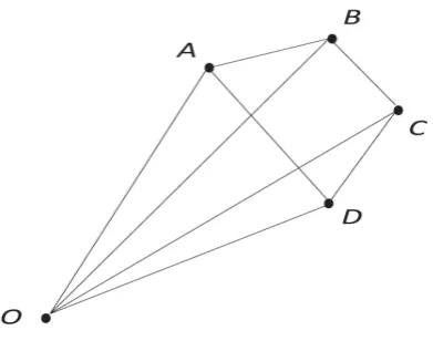
strong supporting and the corresponding face, H∩Tc, is called strong face. Consider DMUo in
Figure 1. Using model (2.3), it can be seen that there are alternative optimal solutions which de-fine an infinite number of supporting hyperplanes passing through DMUo, of which only two
hyper-planes (H1 and H2) are strong and F1= H1
∩
Tc,
F2 = H2
∩
Tc are the strong facets of Tc. We
propose an algorithm for determining all of the FDEFs of Tc. To completely characterize the
structure of the FDEF of Tc, we need the
fol-lowing definitions and preliminaries:
Figure 1: H1 and H2 are defining and H is supporting but not defining.
Definition 3.1 Suppose thatH :U∗ty−V∗tx=
0is a supporting hyperplane ofTc. F = H
∩
Tcis
called a Full Dimensional Efficient Facet (FDEF) of Tc, if (i) there exists at least one affine
inde-pendent set withm+selements of CCR-efficient DMUs lying onF = H∩Tc, and (ii) all
multipli-ers are strictly positive, i.e. (U∗, V∗)>0.
The hyperplane that satisfies the above defini-tion is calledStrong Defining Hyperplane (SDH) of Tc.
Suppose thatH:U∗ty−V∗tx= 0 is a support-ing hyperplane of Tc. If the DMUs (observed or
virtual) (¯x,y¯) and (˜x,y˜) belong to Tc and lie on
H, then the DMU, µ(¯x,y¯) +η(˜x,y˜), belongs to Tc and lies on H for any positive scalars µ and
η. Therefore, the intersection of each supporting hyperplane of Tc with it, is a convex polyhedral
cone. Each convex polyhedral cone is completely characterized by its extreme directions2. So we have the following definitions:
In a given convex set, a nonzero vector d is called a (recession) direction of the set if for each
xo in the set; the ray {xo+λd|λ≥0} also
be-longs to the set. Hence starting at any point xo
in the set, one can recede along d for any step length λ≥0 and remain within the set. An ex-treme direction of a convex set is a direction of the set that cannot be represented as a positive combination of two distinct directions of the set. Two vectors, ¯d and ˜d are said to be distinct or not equivalent, if ¯d cannot be represented as a positive multiple of ˜d.
The following lemma characterizes the extreme directions of the strong face, F = H∩Tc, where
H is a strong supporting hyperplane of Tc.
Lemma 3.1 Suppose that H : U¯ty−V¯tx = 0
is a strong supporting hyperplane of Tc. An
(m+s)−vector,d,is an extreme direction of the strong face,H∩Tc, if and only if it is an extreme
CCR-efficient DMU lying on H.
Proof. Let DMUo = (xo, yo) be an extreme
CCR-efficient DMU that lies on H. Since the set H∩Tc is a convex polyhedral cone, the point
(˜x,y˜) +λ(xo, yo) belongs to the set H
∩
Tc for
any point (˜x,y˜) in the set H∩Tc and any
pos-itive scalar λ. Therefore (xo, yo) is a recession
direction of the set H∩Tc. By contradiction,
we prove that it is also extreme. Otherwise, there exist two distinct recession directions of the set H∩Tc (i.e., two distinct points of the set
H∩Tc), namely, ¯dand ˜d, such that:
(xo, yo) = ¯αd¯+ ˜αd ,˜ α,¯ α >˜ 0.
Since ¯dand ˜dbelong to the H∩Tc, by the
struc-ture of Tc, there exist nonnegative vectors ˜λand
λsuch that ¯
d=
n
∑
j=1
¯
λj(xj, yj)
and ˜
d=
n
∑
j=1
˜
λj(xj, yj) , λ¯j, ˜λj ≥0, f or allj.
Hence,
(xo, yo) = ¯α n
∑
j=1
¯
λj(xj, yj) + ˜α n
∑
j=1
˜
λj(xj, yj)
In other words,∑nj=1λˆjxj =xoand
∑n
j=1ˆλjyj =
yo where ˆλj := ¯α¯λj + ˜αλ˜j, j = 1,2, ..., n. This
relations show that
(
θ= 1,ˆλ
)
is a feasible solu-tion of model (2.1) in evaluating DMUo, in which
for at least some index, t ̸= o, bλt > 0.This is a
contradiction.
On the other hand, suppose that ¯dis an extreme recession direction of the set H∩Tc. Let ¯d =
(¯
dx,d¯y
)
where ¯dx ∈ Rm+ and ¯dy ∈ Rs+. Since
the point ¯d lies on the hyperplane H, we have ¯
Utd¯y−V¯td¯x = 0. Since(U ,¯ V¯)>0, without loss of generality, we can assume that the coefficient vectors(U ,¯ V¯)has been normalized with respect to ¯d, i.e. ¯Utd¯y = ¯Vtd¯x = 1. Therefore, ¯dis CCR-efficient. We evaluate ¯d by model (2.1); In each optimal solution, λ∗, we have
∑
j∈Rd
λ∗jxj = ¯dx,
∑
j∈Rdλ∗jyj = ¯dy,
λ∗j ≥0, j ∈Rd.
Since ¯d belongs to H, by the above relations, DMUj, j∈Rdbelongs to the set H
∩
Tc. So each
DMUj, j∈Rd is also a recession direction of the
set H∩Tc. We claim that ¯dis equal to exactly
one DMUt, t∈ Rd; In other words, equivalently
exactly for one index t ∈ Rd we have λ∗t > 0.
Otherwise, if there is more than one indexj ∈Rd
such that λ∗j >0, then the extreme recession di-rection is written as a nonnegative combination of at least two distinct recession directions of H∩Tc
and this is a contradiction.
We can go further and prove the following theo-rem:
Theorem 3.1 Suppose that H : U∗ty−V∗tx =
0 is a SDH of Tc, i.e., H
∩
Tc is a FDEF
of Tc, then there exists at least one linear
independent set with m + s − 1 elements of extreme CCR-efficient DMUs in the set H∩Tc.
Proof. Since the set H∩Tc is a FDEF of Tc,
there exists at least one linear independent set with m+s−1 elements of CCR-efficient DMUs in the set H∩Tc. Therefore, the set H
∩
Tc is
an (m+s−1)-dimensional convex polyhedral
cone. Suppose that D = {DMU1, ...,DMUk}
is the set of all extreme recession direc-tions of H∩Tc. So H
∩
Tc is equal to all
nonnegative combinations of the elements of the set D, i.e. H∩Tc = P os(D) :=
{∑k
j=1λj DMUj|λj ≥0, j= 1, ..., k
}
. By
Lemma 3.1, each DMUj is an extreme
CCR-efficient DMU. It is clear that k ≥ m+s−1. Since the set H∩Tcis an (m+s−1)- dimensional
convex polyhedral cone, there is some linearly independent (m+s−1)-subset of D, and the result is in hand.
Here we open a question: Suppose that H is an SDH of Tc. Is the set H
∩
Tc a (m+s−
1)-simpilical cone? i.e., does existexactly one linear independent set with m+s−1 elements of the extreme CCR-efficient DMUs lying on H? The answer is negative. The following counterexample illustrates this fact (see Figure 2).
Counterexample
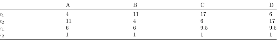
Consider four DMUs are given in Table 1. Units A, B, C and D in Table 1 use two inputs to produce two outputs. By using model (2.4), we can verify that all these DMUs are extreme CCR-efficient. Moreover, all of them lie on the SDH H : 16y1+ 9y2−7x1−7x2 = 0. The
inter-section of H and the PPS constructed by these DMUs is a 3-dimensional FDEF of PPS. As de-picted in Figure 2., indeed, these DMUs are the four extreme directions of this FDEF. This fig-ure visually describes a section at a given output level, sayy2 = 1.
Table 1: Data of counterexample
A B C D
x1 4 11 17 6
x2 11 4 6 17
y1 6 6 9.5 9.5
y2 1 1 1 1
Formulation for Identifying a FDEF: Suppose that H : U∗ty−V∗tx = 0 is a strong support-ing hyperplane of Tc passing through DMUo. As
we mentioned above, the set H∩Tc is a
con-vex polyhedral cone that is generated by its ex-treme recession directions. Let D = {D1, ...,Dk}
be the set of all extreme recession directions of the face H∩Tc, then H
∩
Tc = P os(D) :=
{∑k
j=1λj DMUj|λj ≥0, j= 1, ..., k
}
. Thus, for finding a SDH passing through DMUo, we
should find a strong supporting hyperplane asH:
U∗ty−V∗tx= 0 that it is passing through max-imum number of extreme CCR-efficient DMUs. To do this, we use the following mixed integer lin-ear programming problem, presented in Cooper et al. [18] with small changes:
M in Io=
∑
j∈EIj
s.t. Vtxo = 1,
Utyo= 1,
Utyj−Vtxj+tj = 0 , j ∈E,
tj−M Ij ≤0 , j ∈E,
Ij ∈ {0,1} , j ∈E,
tj ≥0 , j ∈E,
U ≥0 , V ≥0
(3.5)
where the set E is the set of all extreme CCR-efficient observed units and M is a sufficiently large positive quantity.
Note that Ij = 0 if and only iftj = 0, i.e., DMUj
belongs to the hyperplane H :Uty−Vtx+u = 0. Then, since we are minimizing ∑j∈EIj and
Ij ∈ {0,1}, model (3.5) will be directed toward
finding optimal solutions with as many Ij∗ = 0 as possible, i.e., with as many possible t∗j = 0; Equivalently with as many possible extreme re-cession directions which H∩Tc has.
Theorem 3.2 Suppose that DMUo is an
ex-treme CCR-efficient DMU. If there exists at least one SDH passing through DMUo and
(U∗, V∗) is an optimal solution of model (3.5)in which(U∗, V∗)> 0, then Ho : U∗
t
y−V∗tx = 0
is a SDH of Tc.
Proof. Suppose that (U∗, V∗) is an optimal
solution of model (3.5) in which (U∗, V∗) >
0. Since there exists at least one SDH pass-ing through DMUo, by Theorem 3.1 , we have
Io∗ = |E| −k≤ |E| −(m+s−1). Consider the following model:
M ax Utyo
s.t. Vtxo= 1,
Utyj −Vtxj ≤0 , j ∈E,
U ≥0, V ≥0.
(3.6)
In fact model (3.6) is the multiplier form with constraint restricted to j∈E. It is apparent that (U∗, V∗) is an optimal solution of model (3.6). There are two cases:
Case (I). (U∗, V∗) is an extreme (basic fea-sible) optimal solution of model (3.6). Then, because (U∗, V∗) > 0, there exist m +s lin-early independent constraints of Utyj −Vtxj ≤
0 , j ∈ E binding at (U∗, V∗). Suppose that
U∗tyji − V∗ t
xji = 0, i = 1, ..., m + s are
these linearly independent constraints binding at (U∗, V∗). Therefore, the following matrix is row full rank:
−xj1
−xj2
.. .
yj1
yj2
.. .
−xjm+s yjm+s
and it is row equivalent with the following matrix:
−xj1
xj1 −xj2
.. .
yj1
yj2 −yj1
.. .
xj1 −xjm+s yjm+s−yj1
so the set {DM Uji−DM Uj1}
m+s
i=2 is linear
inde-pendent. Hence there exist m+s affinely inde-pendent of extreme CCR-efficient DMUs lying on H∗∩Tc. Therefore, by
Definition 3.2 , H∗∩Tc is a FDEF ofTc .
We prove that this cannot take place. Sup-pose that
(
U1, V1
)
, ...,
(
Uh, Vh
)
are the gradients of all the SDH passing through DMUo, where
(
Ui, Vi
)
> 0, i = 1, ..., h and
(
˜
U1, V˜1
)
, ...,
(
˜
Ul, V˜l
)
are the gradients of all the weak defining hyperplane passing through DMUo. It is clear that
(
Ui, Vi
)
>0, i= 1, ..., h
and
(
˜
Ui,V˜i
)
, i = 1, ..., l are all the extreme optimal solutions (Basic optimal feasible) of model (3.6). Since (U∗, V∗) is not an extreme optimal solution of model (3.6), it can be represented as a convex combination of vectors
(
Ui, Vi
)
> 0, i = 1, ..., h and
(
˜
Ui,V˜i
)
, i= 1, ..., l,. In other words:
(U∗, V∗)
=∑hi=1λi
(
Ui, Vi
)
+∑li=1λ˜i
(
˜
Ui, V˜i
)
∑h i=1λi+
∑l
i=1λei = 1, λi ≥0,
i= 1, ..., h, ˜λi ≥0, i= 1, ..., l.
(3.7) There are two cases:
Case (I). There exists such a combination as (3.7) in which for some index r ∈ {1, . . . , h}, λr ̸=
0. Then, all of the extreme CCR-efficient DMUs lying on H∗o, are also lying onHr:Ury−Vrx= 0 and these DMUs are the only extreme efficient DMUs that are lying on Hr. Because if there exists another extreme CCR-efficient DMU lying on Hr, in addition to these extreme CCR- efficient DMUs lying on H∗o, then (Ur, Vr) is a feasible solution to model (3.5) where its objective value is less than I∗o, and this is a contradiction. Case (II). There is no combination as (3.7) in whichλi > 0 for some index i ∈ {1, . . . , h}. In
other words, in any combination such as (3.7),
λi = 0 for all indices i. Therefore, the strong
face, H∗o∩Tc, is not contained in any FDEF of
Tc. Again, this is a contradiction.
Thus, (U∗, V∗) is an optimal extreme solution of model (3.6) and so is an extreme optimal solution of model (2.3).
Conclusion 1. Suppose that DMUo is an
extreme CCR-efficient DMU and the vector (U∗, V∗) > 0 is an optimal solution of model (3.5), then it is an extreme (basic feasible) op-timal solution of model (2.3) via the simplex
method.
4
The proposed algorithm for
finding all SDHs of
T
cIn this section, using the characterization of structure of FDEFs that is completed in the above exploration, we propose an algorithm for finding all of the FDEFs of Tc.
4.1. The proposed algorithm
Our algorithm performs the following proce-dure for each extreme CCR-efficient DMU in each stage. Main procedure. Consider extreme CCR-efficient observed unit, DMUo, and evaluate it by
model (3.5). Recalling Theorem 3.2, if there ex-ists at least one FDEF containing DMUo
(equiv-alently if there exists at least one SDH passing through DMUo), then the optimal solution of
model (3.5) will be the gradient of a SDH passing through DMUo and it is positive for variables U
and V. If the optimal solution of model (3.5) is notpositive for variablesU and V, then the pro-cedure will be terminated for DMUo. The
pro-cedure implements the following step till the op-timal solution of model (3.5) is positive for vari-ablesU andV.
Main step. Suppose that Io∗ = |E| − k and (U∗, V∗) >0 respectively are the optimal objec-tive and optimal solution of model (3.5). LetHo∗:
U∗ty−V∗tx= 0 and Fo = H∗o
∩
Tc. We save H∗o
as a SDH of Tc and set Jo =
{
j:Ij∗ = 0
}
. In fact, the setJo is the indices of all extreme
CCR-efficient DMUs lying on H∗o. Next, we add the following constraint to the constraints of model (3.5): ∑
j∈Jc o
|Ij| −
∑
j∈Jo
|Ij| ≤Io∗−1 (4.8)
and again we evaluate DMUo by model (3.5).
If there exists another SDH except H∗o passing through DMUo, then Theorem 3.2together with
new added constraint, (4.8), will give the gradient of alternative SDH passing through DMUo as an
alternative optimal solution. We save this SDH and construct the setJo, which are corresponding
to it.
If there does not exist another SDH except H∗o passing through DMUo, then the procedure will
Suppose that the implementation of the pro-cedure is repeated t-steps for DMUo. Therefore,
t SDHs are determined. Note that in final step, model (3.5) will have exactly t new added con-straints corresponding to t SDHs that have been determined in the previous steps. Therefore, after the implementation of the procedure for DMUo,
all the SDHs of Tc passing through it, and all
the extreme CCR-efficient DMUs lying on these hyperplanes will be determined.
After termination of the procedure for DMUo,
the main procedure is performed for another ex-treme CCR-efficient DMU3; In order to prevent the algorithm from giving the gradients of iter-ated SDHs that have been determined in the im-plementation of the algorithm for DMUo, the
con-straint Io = 1 always must be added to the
con-straints of model (3.5) in all subsequent stages. In general, in the implementation of the main procedure for the rth extreme CCR-efficient DMU, the constraints Ij = 1, j = 1, ..., r− 1
corresponding to DMUj, j= 1, ..., r−1, that the
algorithm has been implemented for them up to now, must be added to the constraints of model (3.5).
Note that, at the end of any stage, if the num-ber of remaining extreme CCR-efficient DMUs, which the algorithm has not been implemented for them, is less than m+s, then the algorithm will be automatically terminated.4
By considering the structure of the algorithm, the following theorem, Theorem 3.2, guarantees that the algorithm will give the gradients of all
SDHs of Tc before termination.
Lemma 4.1 Suppose thatDMUpandDMUqare
two extreme CCR-efficient DMUs lying on two distinct SDHs namely Hp and Hq (exclude their
intersection). Then each strict convex combina-tion ofDMUp and DMUq is strong efficient, if it
is not radial inefficient.
Proof. Let DMUl = λDMUp + (1−λ)DMUq
where 0 < λ < 1. Suppose that DMUl is not
radial inefficient, then it is not an interior point of Tc, so it lies on frontier of Tc. If this frontier
3
For computational purposes, it is better to have the algorithm in the next stage implemented for an extreme CCR-efficient DMU that the number of determined SDHs passing through it is less than that of other DMUs.
4
Note that there exist at leastm+s−1 extreme CCR-efficient DMUs on each SDH of Tc(see Theorem3.1).
is strong, we are done. Otherwise it lies on weak frontier. Since DMUp and DMUq also lie on this
frontier, and they belong to the reference set of DMUl, By Theorem 3.4 in [17]- each nonnegative
c1ombination of the elements of reference set is strong efficient- DMUl is strong efficient. This is
a contradiction.
Theorem 4.1 In the implementation of the
mentioned algorithm for DMUo in set E, while
there exists a SDH passing through DMUo, the
optimal solution of model (3.5) for variables U and V will be positive.
Proof. By virtue of the type of the added
constraints through the implementation of algo-rithm, it is sufficient to prove that the optimal solution of model (3.5) for variables U and V
will be positive. By contradiction suppose that the optimal solution of model (3.5), (U∗, V∗), is not positive andIo∗ = |E| − k. Since there ex-ists at least one SDH passing through DMUo,
k ≥ m+s−1. Let R = {DMU1, ...,DMUk} be
the set of all extreme CCR-efficient DMUs lying on Ho∗ : U∗ty−V∗tx = 0. Since H∗o is a weak defining hyperplane, so each DMUj(j = 1, ..., k)
lies on the intersection H∗o with at least one SDHs of Tc. Suppose that H1, ...,Hl are all these SDHs.
There are two cases:
Case (I). There exists some index t(t ∈ {1, ..., l}) such that all DMUj(j = 1, ..., k) lie on
Ht, Then by considering the optimal value of
ob-jective function, there does not exist another ex-treme CCR-efficient DMU lying on Ht. Since Ht
is a SDH passing through DMUo, the set R is
affinely independent. This shows that there are two distinct m+s−1 dimensional hyperplanes -H∗o and Ht- passing through the set R. This is a
contradiction.
Case (II). There exists at least two DMUs in set R, namely DMUpand. DMUq lying on the
inter-section of H∗owith two distinct SDHs of Tcnamely
Hp and Hq, respectively. Since each convex
com-bination of DMUp and DMUq lies on H∗o, then it
is weak efficient. On the other hand by lemma
4.1it is strong efficient. This is a contradiction.
4.2. Computational advantages of the algorithm
determined for each DMUo before
implementa-tion of their algorithms while it is not an easy task without having all of the FDEFs of the PPS. Our proposed algorithm, in comparison with the algorithm presented by Jahanshahloo et al. [6], has several advantages that are summarized as follows:
1. For identifying all of the FDEF of Tc, in
contrast with the algorithm presented in [6] which it should be implemented forall CCR-efficient (extreme and non-extreme) DMUs, our algorithm is just implemented for ex-treme CCR-efficient DMUs.
2. Adding the constraint Io = 1 to the model
(3.5)’ constraints makes the algorithm able to prevent from generating iterated hyper-planes that have been obtained through im-plementation of the procedure for DMUo,
and thisprogressionally decreases the volume of computations stage by stage.
3. As mentioned in Conclusion 1, in the im-plemetation of the procedure for DMUo, in
each step the procedure gives an extreme (basic feasible) optimal solution of model (3.5). Here, unlike the algorithm presented in [6], in which all the extreme optimal so-lutions (positive and nonegative) of model (3.5) must be found, the structure of our algorithm is such that, firstly, all the pos-itive extreme optimal solutions of model (3.5) (corresponding to all of the SDHs that DMUo lies on them) is obtained and then it
automatically terminates for DMUo.
4.3. Summary of the algorithm for identifying all of the SDHs of Tc
Suppose that we have n DMUs, DMUj,
j = 1, 2, ..., n, with input vector xjand
output vector yj. We evaluate these DMUs
by model (2.4). Then, we put the extreme CCR-efficient DMUs in set E, i.e., E :=
{DMUj|DMUjis extreme CCR−efficient DMU}.
Set ET=ϕ and S =ϕ.
Step 1. Put DMUp ∈E−ET and set Sp =ϕ.
Step 2. Evaluate DMUpwith model (3.5). If the
optimal solution, (U∗, V∗), is not positive, then set ET:= ET
∪
{DMUp}, and go to Step 5.
Step 3. For the solution(U∗, V∗), set Jp =
{
j:Ij∗ = 0
}
and Jc p =
{
j:Ij∗ = 1
}
. If |Jp| <
m+s−1, then set ET := ET
∪
{DMUp}, and
go to Step 5; Otherwise put the hyperplane Hp :
U∗ty−V∗tx= 0 into set Sp. SetS := S
∪
Sp.
Step 4. Construct the inequality ∑j∈Jc
p|Ij| −
∑
j∈Jp|Ij| ≤Ip∗−1, and add it to the constraints
of model (3.5) and go to Step 2.
Step 5. Add the constraint Ip = 1 to the
con-straints of model (3.5) and If |ET|>|E| −(m+
s−1) go to Step 1, otherwise the algorithm is terminated and stop.
5
Illustrative example
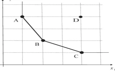
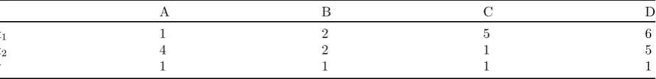
Consider four DMUs, A, B, C and D are given in Table 2 that use two inputs to produce one output. The PPS Tcconstructed by these DMUs
are shown in Figure 3. Clearly all units are
ex-Figure 3: Illustrative example
treme CCR-efficient except unit D. Therefore, ET = {A,B,C}. To give a detailed description
of the algorithm, we implement it stage by stage:
Stage 1:
Let ET =ϕand put A∈E.
Step 1-1. Evaluate unit A by model (3.5). IA∗ =
1 and (v1∗, v2∗, u∗) = (0.3,0.6,1) are respectively the optimal objective and the optimal solution of model (3.5). Since (v1∗, v2∗, u∗) > 0, HA : y−
0.3x1−0.6x2 = 0 is the SDH of Tc; So S ={HA}.
Furthermore, t∗B = 0, that is, HA passes through
B, so set JA ={A,B}, JAc ={C} and construct
the inequality∑j∈Jc A|Ij| −
∑
j∈JA|Ij| ≤I
∗
A−1 =
0 (a1).
Step 1-2. Add the constraint (a1) to the
Table 2: Data of illustrative Example
A B C D
x1 1 2 5 6
x2 4 2 1 5
y 1 1 1 1
model (3.5). We have IA∗ = 2, so the cardinal of the new set JA for A is less than m+s−1 = 2
therefore the algorithm terminates for A. Hence ET ={A} and the set S doesn’t change.
Add the constraint IA = 1 to the constraints of model (3.5) and perform the following stages:
Stage 2:
Step 2-1. Put unit B ∈ E−ET and evaluate
it by model (3.5). IB∗ = 1 and (v1∗, v∗2, u∗) = (0.125,0.375,1) are respectively the optimal ob-jective and the optimal solution of model (3.5). Since (v∗1, v2∗, u∗) > 0, HB : y − 0.125x1 −
0.375x2 = 0 is the SDH of Tc; So S ={HA,HB}.
Furthermore, t∗C = 0, that is, HB passes through
C, so set JB ={B,C}, JBc = {A} and construct
the inequality∑j∈Jc B|Ij| −
∑
j∈JB|Ij| ≤I
∗
B−1 =
0 (b1) .
Step 2-2. Add the constraint (b1) to the
con-straints of model (3.5) and again evaluate B by model (3.5). We haveIB∗ = 2, so the cardinal of the new setJB for B is less than m+s−1 = 2,
therefore the algorithm terminates for B. Hence ET ={A,B} and set S doesn’t change.
Stage 3: Since |ET|>|E| −(m+s−1) = 1, the
algorithm is totally terminated.
6
Conclusion
In this paper, a detailed characterization of FDEFs of Tchas been provided. We have
demon-strated that each FDEF of Tc is a convex
poly-hedral cone which is generated by extreme CCR-efficient DMUs lying on it. In addition, we have proved that the model in Cooper et al. [18] can take part in finding FDEFs. Using this informa-tion, we have proposed an algorithm for identify-ing all FDEFs of Tc. Furthermore, via the
im-plementation of our algorithm, the extreme (ba-sic feasible) optimal solutions of model (2.3) will be automatically generated. As discussed in Sec-tion 4, our algorithm is computationally better than those proposed in [6, 14]. FDEFs may be used in sensitivity and stability analysis,
identi-fying the reference set of a DMU, incorporating performance information into the efficient fron-tier analysis and finding the closest target for a given inefficient DMU. Moreover, in the construc-tion of the cross-efficiency matrix, the gradient of the SDH is the best weight for the CCR-efficient DMUs that lie on it and also for the inefficient DMUs that are projected on it.
References
[1] A. Charnes, W. W. Cooper, E. Rhodes,
Measuring the efficiency of decision making units, European Journal of Operational Re-search 2 (1978) 429-444.
[2] A. Charnes, W. W. Cooper, R. M. Thrall, A structure for classifying and characterizing efficiency and inefficiency in data envelop-ment analysis, Journal of Productivity Anal-ysis 2 (1991) 197-237.
[3] F. Rezai Balf,Ranking Efficient Units by Re-qular Poygon Area (RPA) in DEA, Interna-tional Journal of Mathmatics 3 (2011) 41-54.
[4] F. Rezai Balf, R. Shahverdi, Extension on Regularity Condition in DEA Models, In-ternational Journal of Mathmatics 1 (2009) 227-234.
[5] G. Abri, N. Shoja, M. Fallah Jelodar, Sen-sitivity and Stability Radius in Data Envel-opment Analysis, International Journal of Mathmatics 1 (2009) 227-234.
[6] G. R. Jahanshahloo, A. Shirzadi, M. Mirde-hghan, Finding strong defining hyperplanes of PPS using multiplier form, European Journal of Operational Research 194 (2009) 933-938.
possibility set, European Journal of Opera-tional Research 177 (2007) 42-54.
[8] G. R. Jahanshahloo, F. Hosseinzadeh Lotfi, N. Shoja, M. Sanei, G. Tohidi, Sensitivity and stability analysis in data envelopment analysis, Journal of Operational Research Society 56 (2005) 342-345.
[9] G. Yu, Q. Wei, P. Brockett, L. Zhou, Con-struction of all DEA efficient surfaces of the production possibility set under the general-ized data envelopment analysis model, Eu-ropean Journal of Operational Research 95 (1996) 491-510.
[10] J. Aparicio, J. L. Ruiz, I. Sirvent, Find-ing Closest targets and minimum distance to the Pareto-efficient frontier in DEA tech-nologies, Journal of Productivity Analysis 28 (2007) 209-218.
[11] K. G. Murty,Linear programming, John Wi-ley & Sons, New York, 1983.
[12] M. C. A. Silva, P. Castro, E. Thanassoulis,
Finding closest targets in non-oriented DEA models: the case of convex and non-convex technologies, Journal of Productivity Analy-sis 19 (2003) 251-269.
[13] M. S. Bazaraa, J. J. Jarvis, H. D. Sher-ali,Linear Programming and Network Flows, John Wiley & Sons, New York, 1977.
[14] O. B. Olesen, N. C. Petersen, Identification and use of efficient faces and facets in DEA, Journal of Productivity Analysis 20 (2003) 323-360.
[15] O. B. Olesen, N. C. Petersen, Indicators of ill-conditioned data sets and model misspec-ification in Data Envelopment Analysis: An extended facet approach, Management Sci-ence 42 (1996) 205-219.
[16] R. D. Banker, A. Charens, W. W. Cooper,
Some models for estimating technical and scale inefficiencies in data envelopment analysis, Management Science 30 (1984) 1078-1092.
[17] W. W. Cooper, L. M. Seiford, K. Tone,Data envelopment analysis: A comprehensive text with models, Applications References and
DEA-Solver Software, Springer, New York, 2007.
[18] W. W. Cooper, J. L. Ruiz, I. Sirvent, Choos-ing weights from alternative optimal solu-tions of dual multiplier models in DEA, Eu-ropean Journal of Operational Research 180 (2007) 443-458.
Golam Reza Jahanshahloo is a Professor of Applied Mathemat-ics at Kharazmi (Tarbiat Moallem) University, Tehran, Iran. His re-search interests include linear pro-gramming, multi-objective linear programming problems, and data envelopment analysis. He has supervised many M.Sc and Ph.D students in these areas, and has published many papers in international journals.
Israfil Roshdi was born in the Iran, East Azerbaijan in 1982. He has got M.Sc degree in Ap- plied Math-ematics, Operations Research field in 2007 from Kharazmi (Tarbiat Moallem) University as the top student. He is now a PhD student of Applied Mathematics at Sci- ence and Research Branch, Islamic Azad University. He is working on linear programming, data envelopment analy-sis, and multi-objective linear programming prob-lems.