Vol. 4, No. 4, Year 2012 Article ID IJIM-00201, 9 pages Research Article
Target setting in additive models with preferences
and interval data
Sohrab Kordrostamia∗, Fatemeh Keshavarz Gildeha
(a) Department of Mathematics, Lahijan Branch, Islamic Azad University, Lahijan, Iran
——————————————————————————————————
Abstract
In this paper, the focus is on additive models with interval data.An additive model can be converted to a multi-objective linear problem if information about preferences of the consumption of inputs and the production of outputs are taken into account. Here in this study, data are not exact and are of interval kind. Moreover, the most preferred solutions with available information by interval additive models are sought. It has also been shown that if additional information is available, an axial solution can be applied. Also, the most preferred target settings will be computed too. In this study twenty bank branches in Iran are evaluated, and target settings and efficiency are compared with the original case and significant decisions are made. .
Keywords: Data envelopment analysis; Additive model; Axial solution; Partial information; Inter-val data.
——————————————————————————————————
1
Introduction
Data envelopment analysis is a powerful tool to measure the relative efficiency of each decision making unit. Unlike the original DEA model, we assume further that the levels of inputs and outputs are not known exactly. Hinojosa and M?rmol (2011) introduced an axial solution for MOLP , in which partial information is available. Whenever a group of DMUs has the same objective functions with different weights, we can apply the axial solutions, and then the most preferred solutions are sought among all solutions. Reduction of the number of optimal solutions is the result of this performance. Determination of the target setting becomes difficult in problems with multiple inputs and outputs. In this case, a set of weights has to be determined in order to aggregate the outputs and inputs. The goal is the computation of optimal solutions in an additive model that could be set as target values for a DMU with partial information about preferences.
∗Corresponding author. Email address: [email protected]
Determination of the target setting becomes difficult in problems with multiple inputs and multiple outputs. In this case, a set of weights has to be determined to aggregate the outputs and inputs. The goal is the computation of optimal solutions in additive model that could be as set target values for aDM U with partial information about preferences.
2
MOLP WITH PARTIAL INFORMATION
A multi-objective linear problem in general form is as follows:
maxf(λ) = [f1(λ), ..., fr(λ), ..., fs(λ)]
s.t λ∈Ω
(2.1)
Ω is the feasible set in decision space, and fr : Rn → R1;r = 1, ..., s , are the linear continuous differentiable real value function. The information about preferences is the set of information Λ⊆∆s−1 that ∆s−1 ={α ∈Rs+;∑sr=1αr = 1}.Λ is the set of admissible weights for DM U s. Axial solutions are all λ′s in relation (2−2).
t∗ = max{t∈R;∃λ∈Ω, f(λ)≽Λt∗p (2.2)
P is an improvement axis. Hinojosa and Mrmol (2011) proved that MOLP (2-1) can be transformed to a linear problem, as follows:
maxt
s.t αhf(λ)≥tαhP, h= 1,2, ..., k
λ∈Ω (2.3)
3
AXIAL SOLUTIONS OF TARGET SETTINGS IN AN
ADDITIVE MODEL
Assume we have N decision making units (DM U s), and each one produces n outputs denoted by yrj, and consumes m inputs denoted by xij.
3.1 AN Additive Model
output-oriented additive DEA model for constant return scale technology is
maxs=∑mr=1s+r
s.t. ∑Nj=1λjyrj −s+r =yro; (r= 1, ..., m); ∑N
j=1λjxij ≤xio; (i= 1, ..., n);
λj ≥0; (j= 1, ..., N);s+r ≥0; (r = 1, ..., m)
(3.4)
An additive model doesn’t measure the efficiency value whose job is introducing efficient and inefficient DMUs and determining the target settings.
3.2 An interval additive model
Now if data belong to interval, model (3-4) should be changed, that is should be written as two models to compute the lower and upper bound of objective functions and target set-tings. Models (3-5) and (3-6) are formulated, we consider both input- and output-oriented models.
maxs=∑mr=1sr++∑ni=1s−i
s.t. ∑Nj=1,j̸=oλjyrj+λoyro−s+r =yro ; (r= 1, ..., m); ∑N
j=1,j̸=oλjxij+λoxio+s−i =xio; (i= 1,2, ..., n);
λj ≥0; (j= 1, ..., N);s+r ≥0; (r= 1, ..., m);s−i ≥0; (i= 1, ..., n);
(3.5)
maxs=∑mr=1sr++∑ni=1s−i
s.t. ∑Nj=1,j̸=oλjyrj+λoyro−s+r =yro ; (r= 1, ..., m); ∑N
j=1,j̸=oλjxij+λoxio+s−i =xio; (i= 1,2, ..., n);
λj ≥0; (j= 1, ..., N);s+r ≥0; (r= 1, ..., m);s−i ≥0; (i= 1, ..., n);
(3.6)
3.3 An additive model is converted to MOLP
The objective function of model (3-4) is the equivalent of (3-7):
(∑Nj=1λjy1j−y1o, ∑N
j=1λjy2j−y2o, ..., ∑N
j=1λjynj−yno) (3.7) Therefore model (3-4) is reformulated again to model (3-8).
max(∑Nj=1λjy1j−y1o,∑Nj=1λjy2j −y2o, ...,∑jN=1λjynj−yno)
s.t.∑ ∑Nj=1λjxij ≤xio; (i= 1,2, ..., m); N
j=1λjyrj−yro≥0; (r = 1,2, ..., n);
λj ≥0; (j= 1,2, ..., N);s+r ≥0; (r= 1,2, ..., n);
(3.8)
In DEA models, the improvement axis can be the output vector, and weights of the objective functions are denoted by Model (3-6) is converted to model (3-7), according to (2-3).
maxt
s.t. ∑nr=1αhr∑Nj=1λj(yrj−yro)≥t ∑n
r=1αhryro; (h= 1,2, ..., k); ∑N
j=1λjxij ≤xio; (i= 1,2, ..., m); ∑N
j=1λjyrj−yro≥0; (r = 1,2, ..., n);
λj ≥0; (j= 1,2, ..., N)
We consider both input- and output- oriented models. Now, improvement axis is P = (x1o, ..., xno, y1o, ..., yno) ,for reduction of inputs and increase of outputs. Also the weight vector of the objective function is (αh1, ..., αhn, β1h, ..., βnh).
maxt
s.t. ∑nr=1αhr(∑Nj=1λjyrj−yro) + ∑m
i=1βih( ∑N
j=1−λjxij +xio)≥
t(∑mi=1βihxio+ ∑n
r=1αhryro); (h= 1,2, ..., k); ∑N
j=1λjxij ≤xio; (i= 1,2, ..., m); ∑N
j=1λjyrj ≥yro; (r = 1,2, ..., n);
λj ≥0; (j= 1,2, ..., N)
(3.10)
4
THE MODEL WITH INTERVAL DATA
In this section, we deal with interval data. The exact values of data are not available; the only available information to us is the lower bound and upper bound values. Models (4-1) and (4-2) show the lower and upper objective functions, respectively.
t= maxt
s.t. ∑nr=1αhr(∑Nj=1,j̸=oλjyrj −yro) + ∑n
r=1αhr(λoyro−yro) +∑mi=1βhi(∑Nj=1,j̸=o−λjxij +xio) +
∑m
i=1(−λoxio+xio)≥
t(∑mi=1βh ixio+
∑n
r=1αhryro); (h= 1,2, ..., k); ∑N
j=1,j̸=oλjxij+λoxio ≤xio; (i= 1,2, ..., m); ∑N
j=1,j̸=oλjyrj+λoyro ≥yro; (r= 1,2, ..., n);
λj ≥0; (j= 1,2, ..., N)
(4.11)
t= maxt s.t. ∑nr=1αh
r( ∑N
j=1,j̸=oλjyrj −yro) + ∑n
r=1αhr(λoyro−yro) +∑mi=1βhi(∑Nj=1,j̸=o−λjxij +xio) +
∑m
i=1(−λoxio+xio)≥
t(∑mi=1βihxio+ ∑n
r=1αhryro); (h= 1,2, ..., k); ∑N
j=1,j̸=oλjxij+λoxio ≤xio; (i= 1,2, ..., m); ∑N
j=1,j̸=oλjyrj+λoyro ≥yro; (r= 1,2, ..., n);
λj ≥0; (j= 1,2, ..., N)
(4.12)
5
THE APPLIED EXAMPLE
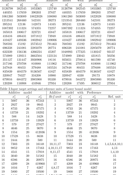
We present an application to target setting in an additive model with interval data involving preferences of objective of each DMU. We apply our approach to some bank branches in Iran (Jahanshahloo.G.R. et all) There are 20 bank branches, each branch produces five outputs by consuming three inputs. Payable interest, personnel and non-performing loans are inputs and the total sum of four main deposits, other deposits, loans granted, received interest and fee are outputs. At first, preferences of objective are not taken into account. Two sets of information about DMUs exist.
Λ1={y4≥y1;y3 ≥y5;y2 ≥ 23y1;y2≥2y3;x2≥x1}
Λ2 ={3y4 ≥2y1;y5 ≥ 12y3;y2 ≥ 34y1;x3 ≥ 12x2} Extreme points of these sets are weights
Table 1.Output target settings of Lower bound model
Additive model Additive model with preference
y1∗ y2∗ y3∗ y∗4 y1∗ y2∗ y∗3 y4∗
3126798 382545 1853365 125740 3126798 382545 1853365 125740
440355 117659 390203 37837 440355 117659 390203 37837
1061260 503089 18822028 108080 1061260 503089 1822028 108080
1213541 268460 542101 39273 1213541 268460 542101 39273
395241 12136 142873 14165 395241 12136 142873 14165
1087392 111324 574355 72257 1087392 111324 574355 72257
165818 180617 323721 45847 165818 180617 323721 45847
416416 486431 1071812 73948 416416 486431 1071812 73948
410427 449336 1802942 189006 410427 449336 1802942 189006
768593 15192 2573512 791463 768593 15192 2573512 791463
696338 241081 2285079 20774 696338 241081 2285079 20774
632339 156136 4266224 45207 1048993 177325 1130247 93137
574989 129311 3662504 122124 574989 23043 431815 50256
351127 131447 3930906 18116 935651 270814 661590 45740
317186 270708 810088 111962 317186 270708 810088 111962
347848 80453 379488 165524 347848 80453 379488 165524
835839 404579 9136507 41827 835839 404579 9136507 41827
320947 78327 334208 10980 320947 6330 29173 10878
679916 684372 3985900 95330 679916 584372 3985900 95330
120208 116908 410946 27934 120208 17495 308012 27934
Table 2.Input target settings and reference units of Lower bound model
Additive model Additive model with Preference
x∗1 x∗2 x∗3 Ref.unit x∗1 x∗2 x∗3 Ref. unit
1 5007 36 87243 1 5007 36 87243 1
2 2927 19 9945 2 2927 19 9945 2
3 8733 26 47575 3 8733 26 47575 3
4 13759 21 19292 4 13759 21 19292 4
5 588 14 3428 5 588 14 3428 5
6 13759 19 13929 6 13759 19 13929 6
7 579 27 27827 7 579 27 27827 7
8 4646 25 9070 8 4646 25 9070 8
9 1554 20 412036 9 1554 20 412036 9
10 17528 15 8638 10 17528 15 8638 10
11 2444 20 500 11 2444 20 500 11
12 7303 23 16148 10,11,17 7303 23 16148 1,4,5,6,8,10,11
13 9852 18 17163 4,10,11,17 9852 18 17163 4,13
14 4541 15 17918 8,11,17 4541 15 17918 1,4,10
15 3040 39 51582 15 3040 39 51582 15
16 6586 26 20975 16 6586 26 20975 16
17 4209 28 419960 17 4209 28 419960 17
18 1016 7 6267 4,8,17 1016 7 6267 18
19 5800 27 19500 19 5800 27 19500 19
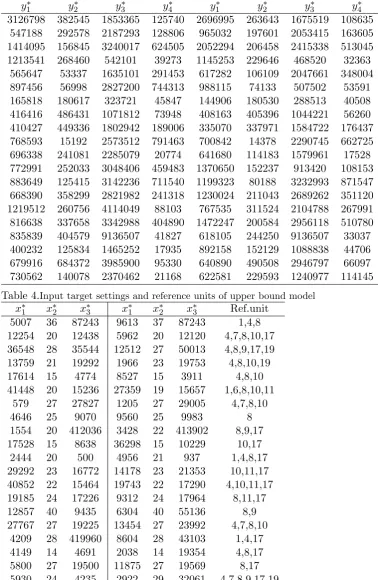
Table 3.Output target settings of upper bound model
y1∗ y2∗ y3∗ y4∗ y1∗ y∗2 y∗3 y∗4
3126798 382545 1853365 125740 2696995 263643 1675519 108635 547188 292578 2187293 128806 965032 197601 2053415 163605 1414095 156845 3240017 624505 2052294 206458 2415338 513045
1213541 268460 542101 39273 1145253 229646 468520 32363
565647 53337 1635101 291453 617282 106109 2047661 348004
897456 56998 2827200 744313 988115 74133 507502 53591
165818 180617 323721 45847 144906 180530 288513 40508
416416 486431 1071812 73948 408163 405396 1044221 56260 410427 449336 1802942 189006 335070 337971 1584722 176437
768593 15192 2573512 791463 700842 14378 2290745 662725
696338 241081 2285079 20774 641680 114183 1579961 17528 772991 252033 3048406 459483 1370650 152237 913420 108153 883649 125415 3142236 711540 1199323 80188 3232993 871547 668390 358299 2821982 241318 1230024 211043 2689262 351120 1219512 260756 4114049 88103 767535 311524 2104788 267991 816638 337658 3342988 404890 1472247 200584 2956118 510780 835839 404579 9136507 41827 618105 244250 9136507 33037 400232 125834 1465252 17935 892158 152129 1088838 44706 679916 684372 3985900 95330 640890 490508 2946797 66097 730562 140078 2370462 21168 622581 229593 1240977 114145
Table 4.Input target settings and reference units of upper bound model
x∗1 x∗2 x∗3 x∗1 x∗2 x∗3 Ref.unit
5007 36 87243 9613 37 87243 1,4,8
12254 20 12438 5962 20 12120 4,7,8,10,17
36548 28 35544 12512 27 50013 4,8,9,17,19
13759 21 19292 1966 23 19753 4,8,10,19
17614 15 4774 8527 15 3911 4,8,10
41448 20 15236 27359 19 15657 1,6,8,10,11
579 27 27827 1205 27 29005 4,7,8,10
4646 25 9070 9560 25 9983 8
1554 20 412036 3428 22 413902 8,9,17
17528 15 8638 36298 15 10229 10,17
2444 20 500 4956 21 937 1,4,8,17
29292 23 16772 14178 23 21353 10,11,17
40852 22 15464 19743 22 17290 4,10,11,17
19185 24 17226 9312 24 17964 8,11,17
12857 40 9435 6304 40 55136 8,9
27767 27 19225 13454 27 23992 4,7,8,10
4209 28 419960 8604 28 43103 1,4,17
4149 14 4691 2038 14 19354 4,8,17
5800 27 19500 11875 27 19569 8,17
DMUs 1,2,3,4,5,6,7,8,9,10,11,15,16,17 and 19 are efficient DMUs in model (3-2) indicating that after accounting the information sets, all of them become efficient. Also all DMUs in model (4-12) are efficient; although efficient DMUs were just 1,4,7,8,9,10 and 11 without accounting preferences. We have compared target settings in both cases (without pref-erences and with prefpref-erences). Target settings are compared between model (4-11) and model (4-12). Also, in this example, we notice that a DMU can become efficient with accounting preferences. These target settings give important and effective information to decision makers when objective function weights are accounted.
6
Conclusion
In this study it has been shown how a manager can be informed about the target settings, so having an inefficient or efficient organization. It is clear that models should be formulated in order to have a better performance, although data may be of the interval kind. The models were performed for a group of Iranian banks. Through using it and with the computation of target settings, a manager diagnoses how to increase outputs or decrease inputs when information about preferences is available.
References
[1] MA Hinojosa, AM. Mrmol, Egalitarianism and utilitarianism in multiple criteria decision problems with partial information, Group Decision and Negotiation doi: 10, (2010)1007/s10726-009-9184-8.
[2] M. Hladik,Generalized linear fractional programming under interval uncertainly, Eu-ropean Journal o Operational Research 3 (2010) 42-46.
[3] M. Hladik, Optimal value range in interval linear programming, Fuzzy Optimization and Decision Making 8(2009) 283-294.
[4] GR. Jahanshahloo, F. Hosseinzadeh Lotfi, M. Rostami Malkhalifeh,MA. Ahadzadeh Namin, generalized model for interval data envelopment analysis with interval data, Applied Mathematical Modelling 33 (2009) 3237-3244.
[5] AM. Mrmol, MA. Hinojosa, Axial solutions for multiple objective linear problems, An application to target setting in DEA models with preferences Omega 39 (2011) 159-168.
[6] AM. Mrmol, J. Puerto, FR. Fernndes,Sequential incorporation of imprecise informa-tion in multiple criteria decision processes, European Journal of Operational Research 137 (2002) 123-133.