Fourth-order numerical solution of a fractional PDE
with the nonlinear source term in the electroanalytical
chemistry
M.ABBASZADE AND A.MOHEBBI1
Department of Applied Mathematics, Faculty of Mathematical Science, University of Kashan, Kashan, Iran
(Received May 13, 2012)
A
BSTRACT
The aim of this paper is to study the high order difference scheme for the solution of a fractional partial differential equation (PDE) in the electroanalytical chemistry. The space fractional derivative is described in the Riemann-Liouville sense. In the proposed scheme we discretize the space derivative with a fourth-order compact scheme and use the Grunwald- Letnikov discretization of the Riemann-Liouville derivative to obtain a fully discrete implicit scheme and analyze the solvability, stability and convergence of proposed scheme using the Fourier method. The convergence order of method is O(τ + ). Numerical examples demonstrate the theoretical results and high accuracy of proposed scheme.
Keywords: Electroanalytical chemistry, reaction-sub-diffusion, compact finite difference, Fourier analysis, solvability, unconditional stability, convergence.
1.
I
NTRODUCTIONIn recent years there has been a growing interest in the field of fractional calculus [6, 16, 22, 26]. Fractional differential equations have attracted increasing attention because they have applications in various fields of science and engineering [4]. Many phenomena in fluid mechanics, viscoelasticity, chemistry, physics, finance and other sciences can be described very successfully by models using mathematical tools from fractional calculus, i.e., the theory of derivatives and integrals of fractional order. Some of the most applications are given in the book of Oldham and Spanier [19] and the papers of Metzler and Klafter [15], Bagley and Trovik [1]. Many considerable works on the theoretical
analysis [5, 25] have been carried on, but analytic solutions of most fractional differential equations cannot be obtained explicitly. So many authors have resorted to numerical solution strategies based on convergence and stability analysis[4, 10, 13, 24]. Liu has carried on so many work on the finite difference method of fractional differential equations [14, 11, 12]. There are several definitions of a fractional derivative of order 0 [22, 19]. The two most commonly used are the Riemann-Liouville and Caputo. The difference between two definitions is in the order of evaluation [18]. We start with recalling the essentials of the fractional calculus. The fractional calculus is a name for the theory of integrals and derivatives of arbitrary order, which unifies and generalizes the notions of integer-order differentiation and n-fold integration. We give some basic definitions and properties of the fractional calculus theory.
Definition 1. For and x 0, a real function f(x), is said to be in the space C if there exists a real number p such that f x( )x f xp 1( ), where f x1( )C(0, ), and for m it is said to be in the space Cm if f mC.
Definition 2. The Riemann-Liouville fractional integral operator of order 0 for a function f (x) C , ≥ -1 is defined as
1 0
0
1
( ) ( ) ( ) , 0, 0, ( ) ( ). ( )
x
J f x x t f t dt
x J f x f x
Also we have the following properties
• ( ) ( ),
• ( ) ( ),
( 1)
• .
( 1)
J J f x J f x
J J f x J J f x
J x x
Definition 3. If m be the smallest integer that exceeds , the Caputo Riemann-Liouville fractional derivatives operator of order 1 is defined as, respectively,
, ,
) (
, 1
, )
( )
( ) (
1
)
( 0
1
0
m dx
x f d
m m m
dt t x dx
x f d t
x m
x f D
m m
x
m m m
t C
. , ) ( , 1 , ) ( ) ( ) ( 1 ) ( 0 1 0 m dx x f d m m m t d t f t x m dx d x f D m m x m m mt (1.2)
Due mainly to the works of Oldham and his co-authors [7, 8, 9, 20, 21], electrochemistry is one of those fields in which fractional-order integrals and derivatives have a strong position and bring practical results. Although the idea of using a half-order fractional integral of current, 0Dt-1/2i(t), can be found also in the works of other authors, it was the paper by
Oldham [20] which definitely opened a new direction in the methods of electrochemistry called semi-integral electroanalysis. One of the important subjects for study in electrochemistry in the determination of the concentration of analyzed electroactive species near the electrode surface. The method suggested by Oldham and Spanier [21] allows, under certain conditions, replacement of a problem for the diffusion equation by a relationship on the boundary (electrode surface). Based on this idea, Old ham [20] suggested the utilization in experiment the characteristec described by the function
1 2 0
( )
t( )
m t
D
i t
which is the fractional integral of the current , as the observed function, whose values
can be obtained by measurements. Then the subject of main interest, the surface concentration Cs(t) of the electroactive species, can be evaluated as
), ( ) ( 2 1 0
0 k D i t
C t
Cs t
(1.3) where k is a certain constant described below, and C0 is the uniform concentration of the electroactive species throughout the electrolytic medium at the initial equilibrium situation characterized by a constant potential, at which no electrochemical reaction of the considered species in possible. The relationship (1.3) was obtained by considering the following problem for a classical diffusion equation [9]
Where D is diffusion coefficient. A is the electrode area, F is Faraday's constant and is the number of electrons involved in the reaction, the constant in (1.3) is expressed as
. 1
D AF n k
Instead of the classical diffusion equation (1.4), it is possible to consider the fractional order diffusion equation [23]
( , ) ( , ) , 2 2 1 0
x t x C D
t t x C
t (1.5)
where 0 1. In this paper, we consider the generalized form of the Eq. (1.5) with the nonlinear source term and on a bounded domain with the following form
, 0
, 0
), , , ) , ( ( ) , ( ) , ( )
, (
2 2
2 1 1 0
T t L
x
t x t x u f t x u x
t x u D
t t x u
t
(1.6)
The boundary and initial conditions are
1 2
(0, ) ( ), ( , ) ( ), 0 ,
u t
t u L t
t t T (1.7)( , 0) ( ), 0 .
u x
x x L (1.8)where 0 1, 1 0, 2 0 and the source term 1 ( , , ) [0, ].
f u x t C L The symbol
1 0Dt
is the Riemann-Liouville fractional derivative operator and is defined as
1
0 1
0
1 ( , )
( , ) ,
( ) ( )
t
t
u x
D u x t d
t t
Where (.) is the gamma function. Also, let f u x t( , , ) satisfies the Lipschitz condition with respect to :
u u u
u t
x u f t x u
f( , , ) (~, , ) ~ , ,~
with the spatial accuracy of fourth order using matrix analysis. The outline of this paper is as follows. In Section 2, we introduce the derivation of new method for the solution of Eq. (1.6). This scheme is based on approximating the time derivative of mentioned equation by a scheme of order O( ) and spatial derivative with a fourth order compact finite difference scheme. In this section we obtain the matrix form of the proposed method and show the solvability of it. In Section 3 we prove the unconditional stability property of method. In Section 4 we present the convergence of method and show that the convergence order is
4
( h )
O . In Section 5 we report the numerical experiments of solving Eq. (1.1) with the
method developed in this paper for several test problems. Finally concluding remarks are drawn in Section 6.
2.
D
ERIVATION OFM
ETHODFor positive integer numbers and , let h=L/M denotes the step size of spatial variable, , and τ = T / N denotes the step size of time variable, . So we define
, 0,1, 2,..., ,
, 0,1, 2,..., . j
k
x jh j M
t k
k N
The exact and approximate solutions at the point (xj,tk) are denoted by ukj and Ukj respectively. We first state the fourth-order compact scheme of second derivative in the following lemma.
Lemma 1([4]). The fourth-order compact difference operator with maintaining three point stencil to approximate the uxxis
2 2 4
4 6
2 4
2 2
1
( ),
1 240
1 12
k k
k x
j
j j
x
u u
u h h
x x
h
O (2.1)
in which 2
1 1
( 2 ).
xuj uj uj uj
[ / ]
1 (1 )
0 1 0 1 ( ) ( ) ( ), t p t k k
D f t f t k
O (2.2)Where (1 )
k
k are the coefficients of the generating function, that is,
( ) 0
( , ) k k k
z z
We will discuss the case for ( , )z (1 z) and thus p=1. Inthis case the coefficients are ( ) ( ) 0
( 1) ( 1)
1 ( 1) ( 1)
! k k k k and k k
for
1
k and can be evaluated recursively,
. 1 , 1 1 ,
1 ( 1)
) ( )
(
0
k
k k
k
(2.3)
Now, we put
(1 ) 1
( 1)l , 0,1, , .
l l l k
l
So 0 1. If we consider Eq. (1.6)-(1.8) at the point (xj,tk), we can write
). , ), , ( ( ) , ( ) , ( ) ( ) , ( 2 2 2 1 1
0 j k j k j k
k j t k j t x t x u f t x u x t x u D t t x u (2.4)
Since f u x t( , , ) has the first order continuous derivative it follows that
. ) ( ) , ), , ( ( ) , ), , (
(u x t x t f u x t 1 x t 1 O f j k j k j k j k
Also, we can write
, ) ( ) , ( ) , ( ) ,
( 1
O t x u t x u t t x
u j k j k j k
, ) ( ) , ( ) , ( 12 1
1 2 4
2 2 2 2 h O h t x u x t x
u j k x j k
x
, ) ( ) , ( ) , ( 2 1 2 0 1 2 2 1
0
O x t x u x t x u
D j k
1 1 0
0
(
,
)
(
,
)
( ),
k
t j k l j k
l
D
u x
t
u x
t
O
From Eq. (2.4) and above results, we can obtain
2 2 2
1 1
0
2 2 1
2 0
1 1
1 ( , ) 1 ( , ) ( , )
12 12
1 1
1 ( , ) 1
12 12
k
x j k x j k l x j k l
l
k
k k
l x j k l x j j
l
u x t u x t u x t
u x t f R
(2.5)
where, 1 1 2 , 2 2 ,
h
and
2 2 4
1 0
1
( ) 1 ( ) .
12
k k
j x l
l
R O
O h
(2.6)By omitting the small term Rkj , the implicit compact difference scheme for (1.6)-(1.8) is given as follows:
2 2 1
2 1 2
2 1 1 2 1 1
2 2 2 1
1 2
2 2
0
0 1 2
1 1
1 1
12 12 12 12
1 1
1 1 ,
12 12
( ), 1, 2, , 1,
( ), ( ), 1, 2, , .
k k
x j x j
k k
k l k l k
l x j l x j x j
l l
j j
k k
k M k
U U
U U f
U x j M
U t U t k N
(2.7)
Now we denote the solution vector of order at t tk by
1 1
( ) ( , , )
k k k T
k M
t U U
1
0
, 1, 2,3, , , k
k l k
l l
A B k N
U U F (2.8)
in which
2
1
2
1
2
11 5 1
1 , 1 2 , 1 ,
12 6 12
tri
A
2 2
1 1 2 1
5
, 2 , ,
12 6 12
l ltri
B
1 1 2 1 2 1 2
1 5 1
1 , 1 , 1 ,
12 6 12
k tri
B
2 1
2 1 0 1 1 2 1 0
2 1
2
2 1
2
2 1
2 1 1 1 2 1
1 1 1
1 1 1
12 12 12
1 1
12
1 1
12
1 1 1
1 1 1
12 12 12
k k k
x
k x
k
k
x M
k k k
M x M M
U f U
f f
U f U
F ,
where tri a a a[ 1 2 3 (]M 1) (M1) denotes a (M 1) (M 1) tri-diagonal matrix. Each row of this matrix contains the values a a1, 2 and a3 on its sub-diagonal, diagonal and super diagonal, respectively. We can state the solvability of proposed scheme in the following theorem.
Theorem 1. The compact difference scheme (2.7) has a unique solution.
3.
S
TABILITY OFP
ROPOSEDM
ETHODIn the section we will analyze the stability of the finite difference scheme (2.7) by using the Fourier analysis. For x = ( x1, x2, …, x-1)T -1 , we define a discrete l2-norm by
2 1 1 1 2 ) ( 2
M j j k x h x . Let
k j
U~ be the approximate solution of (2.7) and define
, ,..., 1 , 0 , ..., , 1 , 0 , ~ M j N k U Ukj kj k
j
with corresponding vector
1 , 2, , 1
.T
k k k k
M
We obtain the following round off error equation
, 1 , 1 1 , ~ 12 1 1 12 1 1 12 12 1 1 ) 12 12 1 ( 1 1 1 2 2 2 2 2 2 1 1 2 2 1 1 1 2 1 2 2 1 2 N k M j ffjk jk
x l k j k l x l k l l k j x l k j x k j x
(3.1) with 0 0. k k M in which f~jk1 f(U~kj1,xj,tk1) We define the grid function
,
2 2
( )
0 0 .
2 2
k
j j j
k
h h
x x x
x
h h
x or L x L
We can expand the k( )x in a Fourier series [5]
2 /
( ) ( ) , 1, 2, , ,
k i lx L
k l
x d l e k N
where
2 / 0
1
( ) L k( ) i lx L .
k
d l x e dx
L
Also we introduce the following norm
. )
( 2
1
0
2 2
1 2 1 1
2
L k M
j k j k
dx x
h
By applying the Parseval equality
, ) ( )
(
2
0
2
l k
L k
l d dx
x
we obtain
2 ( ) 2.
2
l k k
l d
(3.2)
Now we can suppose that the solution of equation (3.1) has the following form
,
k i jh j
d e
k
where 2 l L
. Substituting the above expression into (3.1) and putting h, we
obtain
k
l
k j k j x k
l
k d f f
d
2
2 1
~ 12
1 1
1
(3.3)
where
2 2 2 2
1 2
2 2 1 2 2
1 1 1 2
2 2 2
1 2
1 2 2
cos 4 sin cos ,
3 2 2 3 2 3 3
1 2 2
ˆ cos 4 sin cos ,
3 2 2 3 2 3 3
2
4 sin cos .
2 3 2 3
Lemma 2([14]). The coefficients l satisfy
0 1
0 1
(1) 1, 1, 0, 1, 2, ,
(2) 0, 1, .
l n l l l l l n N
Lemma 3. The coefficient in (3.4) satisfies in 0 1 3
.
Proof. Since 1 and 2 are positive so from (3.4) we can write
2 2 2
1 2 2
1 3 cos 12 sin cos 2 2,
2 2 2
which gives 0 1 3.
Proposition 1. Suppose that dk(1 k N) are defined by (3.3), then we have
. , . . ,. 2 , 1 , ) 3 1
( L d0 k N
dk k
Proof. We will use mathematical induction to complete the proof. For k 1, from (3.3) and using Lemma 3 we can write
. ) 3 1 ( ˆ 12 1 1 ˆ 1 ~ 12 1 1 ˆ 1 ~ 12 1 1 ˆ 1 0 0 0 2 0 0 0 2 0 0 0 2 0 1 d L d L e d L e d U U L e d f f e d d ij ij x j j ij x j j ij x Now suppose . 1 ,..., 2 , 1 , ) 3 1
( 0
L d n k
From (3.3) and induction hypothesis, we can write
2 2 1 1
0 1 0 ~ 12 1 1 1 ˆ ) 3 1
( x ij jk jk
k
l k l
k
k L e f f
d
d
kj k j ij x k l l k k U U L e L d ~ 12 1 1 1 ) ( ˆ ) 3 1
( 1 2
1
0 1
0
ij k ij x k l l k e d L e L d 1 2 1 1 1 0 12 1 1 1 ) ( ˆ ) 3 1 (
L L
d k
0 (1 3 ) 1 ˆ (1 (1 ))
, ) 3 1
( L k d0
which completes the proof.
Theorem 2. The compact difference scheme (2.7) is unconditionally stable for any
0 1.
Proof. Applying Proposition 1 and Parseval's equality, we obtain
, ~ ) 3 1 ( ~ 1 1 2 0 0 3 2 0 3 2 0 1 1 3 2 0 1 1 2 2 1 1 2 1 1 2 2 2 2 2 2
M j l LT l LT jh i M j Lk k M j k M j jh i k M j k j l k l k k U U e e e d e h d L h d h e d h h U U which means that the scheme (2.7) is unconditionally stable.
4.
C
ONVERGENCE OFP
ROPOSEDM
ETHODLemma 4([2]). Regarding to the definitions of l, we have
1 0
1
( ). ( )
k l l
OOn the basis (2.6) and Lemma 4, we have
2 2 4
1 0
2 4 1
1 0
2 4 2 4
1 1
( ) 1 ( )
12
( ) ( )
1
( ) ( ) ( ) ( ),
( )
k k
j x l
l
k l l
R h
h
h h
O O
O O
O O O O
(4.1)
so from (4.1), we can obtain
2 4
( ),
1, 2, , , 1, 2, , ,
k j
R O h
k N j M
therefore, there is a positive constant C1, such that [3]
2 4
1( ).
k j
R C
h (4.2)Similar to the stability analysis in Section 3, we define the grid functions [3]
when , 1, 2, , 1,
2 2
( )
0 when 0 ,
2 2
k
j j j
k
h h
e x x x j M
e x
h h
x or L x L
when , 1, 2, , 1,
2 2
( )
0 when 0 ,
2 2
k
j j j
k
h h
R x x x j M
R x
h h
x or L x L
Thus ek( )x and Rk( )x have the following Fourier series expansions
2
( )
( )
,
0,1,
,
,
i lx
k L
k l
e
x
l e
k
N
2
( )
( )
,
0,1,
,
,
i lx
k L
k l
R
x
l e
k
N
where
2
0
1
( )
( )
,
0,1,
,
,
L i lx
k L
k
l
e
x e
dx
k
N
L
2
0
1
( )
( )
,
0,1,
,
.
L i lx
k L
k
l
R
x e
dx
k
N
L
Now, we define the following notations [3]
( , ) ,
1, 2, , , 1, 2, , ,
k k k k
j j k j j j
e u x t U u U
k N j M
(4.3)
1
,
2,
,
1,
1,
2,
,
1,
1, 2,
,
,
k k k k k k k k
M M
e
e
e
e
R
R
R
R
k
N
and introduce the following norms
1 1
1 2 2 2 2
2
1 0
( ) , 0,1, , , L
M
k k
j j
e h e e x dx k N
1 1
1 2 2 2 2
2
1 0
( ) , 0,1, , .
L M
k k
j j
R h R R x dx k N
(4.5)Using the Parseval equality
L
l x k
N k
l d
x e
k
0
2 2
, , , 1 , 0 ,
) ( )
(
and
2 2
0
( ) ( ) , 0,1, , , L
k
k l
R x dx
l k N
we also have
2 2
2 ( ) , 0,1, , ,
k
k l
e
l k N
(4.6)2 2
2 ( ) , 0,1, , .
k
k l
R
l k N
(4.7)From (2.6), we obtain that
2 2 1 2
1 0
2 2 1
2 0
1 1
1 1
12 12
1 1
1 1
12 12
1, 2, , , 1, 2, , ,
k
k k k l
x j x j l x j
l
k
k l k k
l x j x j j
l
u u u
u f R
k N j M
(4.8)2 2 1 2 1
0
2 2 1
2 0
0 0
1 1
1 1
12 12
1 1
1 1
12 12
0, 0, 1, 2, , , , 1, 2, , .
k
k k k l
x j x j l x j
l
k
k l k k
l x j x j j
l
k k
M j
e e e
e f R
e e e k N j M
(4.9)Now we assume that ekj and Rkj are
( )
( )
, ,
k i jh
j k
k i jh
j k
e e
R e
where 2l L
. Substituting the above relations into (4.9) results
2 2
1 ˆ 1
1 ,
12
1, 2, , .
k
ij k k
k l k l x j j k
l
e f f
k N
(4.10)
Notice that 0 0
e and we have
0 0( )l 0.
In addition, from the left hand equality of (4.5) and (4.2), we obtain [3]
2 4
2 4
1 1
2 .
k
R MhC h C L h (4.11)
Also from convergence of the series in the right hand side of (4.7), there is a positive constant C2 such that [3]
. , , 2 , 1 ,
) ( )
(n C2L 1 C2L 1 n k N
k
k
(4.12)
Proposition 2. If k (k 1, 2,,N) be the solutions of equation (4.10), then there is a positive constant C2 such that
2
1 3
1,
1, 2, , .
k
k
C k
L
k
N
Proof. We use the mathematical induction for proof. Firstly, from (4.10) and (4.12) we have . ) 3 1 ( 3 3 1 1 2 1 2 1 2 1 2 1
1
C L C L C L C L
Now, suppose that
1 , , 2 , 1 , ) 3 1 ( 1
2
C n L n n k
n
From Lemma 2 and noticing that ˆ 0 we have,
. ) 3 1 ( ) 3 1 ( ˆ ) 3 1 ( ) 1 ( ) 3 1 ( ˆ ) 3 1 ( ) 1 ( ) 3 1 ( ˆ ) 3 1 ( ) 1 ( 3 ˆ ) 3 1 ( ) 1 ( 12 1 1 1 ˆ ) 3 1 ( ) 1 ( 1 2 1 2 1 1 2 1 2 1 1 2 1 2 1 1 1 1 2 1 2 1 1 1 0 1 2 1 2 2 1 2 0 1 2 k k k k k k k l l k k l l k k k j k j x ij k l l k k k L C k C L L L k C C L L L k C C L L L k C L C L L k C L C f f e L k C
Theorem 3. Suppose u x t( , ) is the exact solution of the Eq. (1.6), then the compact finite difference scheme (2.7) is L2-convergent with convergence order O( h4).
Proof. By considering Proposition 2 and noticing (4.6), (4.7) and (4.11), we can obtain . ) ( ) 3 1
( 1 2 3 4
2 1 2
2 C k L R C LC ke h
Since k T , we have
4
2
k
e C h
in which
3
1 2 ,
T
C C T Le
L
C
and this completes the proof.
5.
N
UMERICALR
ESULTSIn this section we present the numerical results of the new method on several test problems. We tested the accuracy and stability of the method described in this paper by performing the mentioned scheme for different values of h and . We performed our computations using Matlab 7 software on a Pentium IV, 2800 MHz CPU machine with 2 Gbyte of memory. We calculated the computational orders of the method presented in this article in time variable with [17, 24]
1 2
(2 , )
C -order log ,
( , )
L h
L h
and in space variables with [4]
2 2
(16 , 2 )
C -order log .
( , )
L h
L h
5.1 Test problem 1.
We consider the fractional linear PDE
2 1
0 2
( , ) ( , )
( , ) (1 ) x , t
u x t u x t
D u x t e t
t x
(5.1)
1 1 0
0
,
,
1, 2,
,
,
0,
1, 2,
,
.
k k L
M
j
u
t
u
e t
k
N
u
j
M
(5.2)
Then, the exact solution of (5.1), (5.2) is
1
( , )
x.
u x t
e t
We solve this problem with the method presented in this article with several values of ,
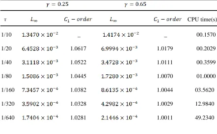
and for at final time . The Lerror, C1-order, C2-order and CPU time (s) of applied method are shown in Tables 1,2.
Table 1. Errors and computational orders obtained for test problem 1 with
CPU time(s)
1/10 _ _ 00.1570
1/20 1.0617 1.0179 00.2029
1/40 1.0522 1.0111 00.3599
1/80 1.0445 1.0070 01.0000
1/160 1.0382 1.0044 03.5620
1/320 1.0328 1.0029 12.9840
1/640 1.0281 1.0011 49.2340
Tables 1,2 show that the computational orders are close to theoretical orders, i.e the order of
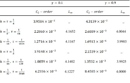
Table 2. Errors and computational orders obtained for test problem 1.
_ _
4.1652 4.0044
4.1167 3.9903
_ _
4.1402 3.9925
4.1227 4.0000
5.2 Test problem 2.
We consider the fractional PDE with the nonlinear source term
2 1
0 2
1
3 2 6 2
( , ) ( , )
( , )
2
( , ) cos( ) 2 ( 1) cos ( ) ,
(2 )
t
u x t u x t
D u x t
t x
t
u x t x t t x
with boundary and initial conditions
2 2
0
0
, cos( ), 1, 2, , ,
0, 1, 2, , .
k k
M
j
u t u t L k N
u j M
where, the exact solution is
2
( , ) cos( ).
We solve this problem with the method presented in this article with several values of
,
h and for L 1 at final time T 1. The L error, C1-order, C2-order and CPU time (s) of applied method are shown in Tables 3, 4.
Table 3. Errors and computational orders obtained for test problem 2 with .
CPU time(s) 1/10 _ _ 00.1250
1/20 0.9758 0.9682 00.1879
1/40 0.9880 0.9844 00.4070
1/80 0.9942 0.9923 00.8279
1/160 0.9974 0.9965 02.9059
1/320 0.9993 0.9988 10.5940
1/640 1.0008 1.0003 41.3440
Tables 3, 4 show that the computational orders are close to theoretical orders, i.e the order
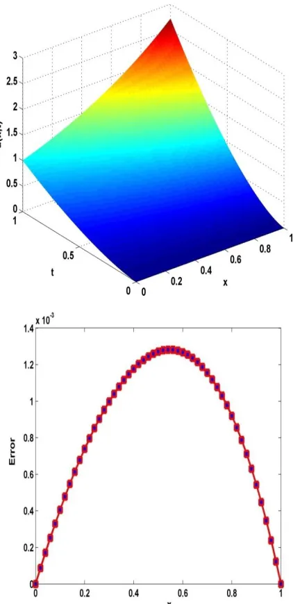
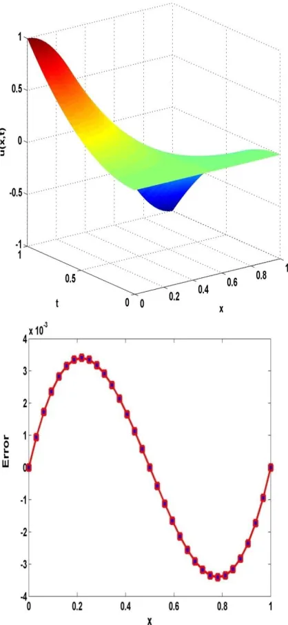
of method is O( ) in time variable and O(h4) in space variables. Figure 1 shows the plots of error and approximate solution of this test problem with h 1/ 32, 1/100 and
Table 4. Errors and computational orders obtained for test problem 2.
_ _
3.9094 3.8537
3.9942 3.9913
_ _
3.9540 3.9284
3.9716 3.9702
6.
C
ONCLUSIONIn this article, we constructed a compact difference scheme for the solution of a fractional nonlinear PDE in the electroanalytical chemistry. This compact difference scheme has the advantage of high accuracy and unconditional stability which we proved it using the Fourier analysis. Also we show that the proposed compact finite difference scheme converges with the spatial accuracy of fourth-order. Numerical results confirmed the theoretical results of proposed method.
R
EFERENCES1. R. Bagley and P. Torvik, A theoretical basis for the application of fractional calculus to viscoelasticity, J. Rheol. 27 (1983) 201210.
3. C. M. Chen, F. Liu and V. Anh, Numerical analysis of the Rayleigh-Stokes problem for a heated generalized second grade fluid with fractional derivatives, Appl. Math. Comput. 204 (2008) 340351.
4. M. Cui, Compact finite difference method for the fractional diffusion equation, J. Comput. Phys. 228 (2009) 77927804.
5. K. Diethelm and N. J. Ford, Analysis of fractional differential equations, J. Math. Anal. Appl. 265 (2002) 229248.
6. R. Du, W. R. Cao and Z. Z. Sun, A compact difference scheme for the fractional diffusion-wave equation, Appl. Math. Model. 34 (2010) 29983007.
7. M. Goto and K. B. Oldham, Serniintegral electroanalysis: studies on the neopolarograrns plateau, Anal. Chem. 46 (1973) 15221530.
8. M. Goto and D. Ishii, Semidifferential elertroanalysis, J. Electroanal. Chem. and Interfacial Electrochem. 61 (1975) 361365.
9. M. Grenness and K. B. Oldham, Semiintegral electroanalysis: theory and verification, Anal. Chem. 44 (1972) 11211129.
10.T. A. M. Langlands and B. I. Henry, The accuracy and stability of an implicit solution method for the fractional diffusion equation, J. Comput. Phys. 205 (2005) 719736.
11.F. Liu, V. Anh and I. Turner, Numerical solution of the space fractional Fokker-Planck equation, J. Comput. Appl. Math. 166 (2004) 209219.
12.F. Liu, C. Yang and K. Burrage, Numerical method and analytical technique of the modified anomalous sub-diffusion equation with a nonlinear source term, J. Comput. Appl. Math. 231 (2009) 160176.
13.Q. Liu, F. Liu, I. Turner and V. Anh, Finite element approximation for a modified anomalous Sub-diffusion equation, Appl. Math. Model. 35 (2011) 41034116. 14.F. Liu, P. Zhuang, V. Anh, I. Turner and K. Burrage, Stability and convergence of
the difference methods for the space-time fractional advection-diffusion equation, Appl. Math. Comput. 191 (2007) 1220.
15.R. Metzler and J. Klafter, The restaurant at the end of the random walk: recent developments in the description of anomalous transport by fractional dynamics, J. Phys. A 37 (2004) R161208.
16.K. S. Miller and B. Ross, An introductional the fractional calculus and fractional differential equations, New York and London, Academic Press, 1974.
17.A. Mohebbi and M. Dehghan, The use of compact boundary value method for the solution of two-dimensional Schröodinger equation, J. Comput. Appl. Math. 225 (2009) 124134.
19.K. B. Oldham, J. Spanier, The Fractional Calculus, Theory and Application of Differentiation and Integration to Arbitrary Order, Academic Press, 1974.
20.K. R. Oldham, A signal-independent electroanalytical method, Anal. Chenl. 44 (1972) 196198.
21.K. B. Oldham and J. Spanier, The replacement of Fick's law by a formulation involvirig semidifferentiation, J. Electroanal. Chem. Interfacial Electrochem. 26 (1970) 331341.
22.K. B. Oldham and J. Spanier, The fractional calculus. New York and London, Academic Press, 1974.
23.I. Podulbny, Fractional differential equations, New York, Academic Press, 1999. 24.A. Saadatmandi and M. R. Azizi, Chebyshev finite difference method for a
two-point boundary value problems with applications to chemical reactor theory, Iranian J. Math. Chem. 3 (2012) 17.
25.Z. Z. Sun and X. N .Wu, A fully discrete difference scheme for a diffusion-wave system, Appl. Numer. Math. 56 (2006) 193209.