1408
Damià Rey Miró
1, AFMJ Volume 3 Issue 03 March 2018
Volume 3 Issue 03 March- 2018, (Page No.-1408-1428)
DOI:10.18535/afmj/v3i3.08, I.F. - 4.614
© 2018, AFMJ
Financial Quality Index (FQI): A New Index to Assess Financial Market
Quality
Damià Rey Miró
1, Pedro V. Piffaut
2, Ph.D.
1
Barcelona Stock Exchange Studies (BME)
Department of Economics, Universidad de Barcelona C/segle XX nº1 Àtic 1 08041, Barcelona, España
2Managing Director of Langeron Econometrics, 156 West 56th Street 10th Floor, New York, NY 10019, USA
Corresponding Author: Damià Rey Miró
Department of Economics, Universidad de Barcelona C/segle XX nº1 Àtic 1 08041, Barcelona, España
Abstract:
Once the financial crisis started in the middle of 2007, the financial authorities and governments of developed economies, based on the premises of the market's security, efficiency and transparency towards investors, began to emphasizethe importance of estimating the systemic risks over the risk of a given sector. Beyond macroeconomic strength, if they have higher quality equity markets, countries should be better prepared to cope with potential volatility. The current work develops a new index (FQI) that shows, in an objective way, the degree of maturity and market stability, in particular for the Spanish equity market1.Keywords:
Stress index, composite indicator, real economy, systemic risk, financial quality index, VAR analysis, econometrics1. Introduction
The crisis that began in the aftermath of Lehman Brothers' collapse has heightened the perception of risk among the financial community. The intervention and coordination between the different central banks and international institutions brought an unprecedented event to safeguard the financial system.
Several studies have tried to capture the degree of systematic risk in the market. The task of detecting and measuring market stress through various indicators has been a significant step forward in improving the functioning of financial markets. There are several types of research that try to measure the stress of financial markets. In Spain for instance, recently the CNMV has developed a work titled "Spanish Financial Market Stress Index (FMSI)", very similar to the work titled "Composite Indicator of Systemic Stress" inspired by Holló, Kremer and Lo Duca. The current research work intends to give a complementary approach to that carried out by the financial community. Therefore, this study is not intended to capture stress or systematic risk, but rather to capture, with maximum objectivity, the financial quality over a particular segment of the financial market. The aim is to improve transparency and, above all, to improve investor protection. It is also intended to facilitate the access of small businesses to financing, as well as to improve aspects of negotiation in certain markets, another of the objectives embodied in MiFID II.
Thus, the current work aims to develop an index that includes relevant parameters of the financial market showing more information to investors and companies when accessing the Spanish market. To this end, the work has focused on the Spanish equities market, where the goal is to replicate the index in other segments in order to improve transparency in relation not only to negotiation, but also to reinforce supervision and improvement of the functioning of the market. Therefore, the present paper and the proposed index could be considered as a major improvement in assessing market quality; an index that can also be replicated to other financial markets.
The paper has been structured in five main sections. The first one shows the existing academic literature and explains the motivation behind conducting the research. The second and third sections are to provide a definition and the aggregation of the indicator with all the sub-indexes, in order to study each of the segments that have been considered relevant in order to capture the quality of the market. Contrasting and identifying past episodes to see the evolution of the quality of the financial market, has been fundamental to shape the evolution of the market itself.
It is clear that the Spanish stock market is among the most developed in the world. Values such as security, solvency, and efficiency are crucial to the functioning of the market. Ensuring transparency and most important, the formation of the price that
1 The authors would like to thank Dr. Joan Hortalá, President of the Barcelona Stock Exchange(a)Domingo García, Director of the
1409
Damià Rey Miró
1, AFMJ Volume 3 Issue 03 March 2018
allows thousands of investors to access the market in conditions of equity, are key aspects for the development of an efficient market. Once these bases are founded, which are not few, the objective turns into showing the average progress of a market by developing a composite indicator that evaluates both the primary and secondary markets as a whole. In the fourth section, because it is necessary that the captured dimensions and their aggregate have a predictive character, an econometric study is carried out through the Markov-Switching models, VAR analysis and other complementary analyzes with the objective of reflecting the robustness of the proposed index formulation. In the fifth and final section, main conclusions and issues are drawn from this research.
2. Existing Literature
Unleashed by the economic crisis that began in mid-2007, financial authorities, as well as governments in the major economies of the developed world, began to emphasize the importance of anticipating and estimating systemic financial risks over risks of a particular sector, such as the banking sector and financial institutions. This is how the IMF, the Financial Stability Board (FSB) and the Bank for International Settlements (BIS) established an approach to assess the systemic importance of markets, financial instruments and financial institutions (IMF-International Monetary Fund, BIS-Bank for International Settlements and FSB-Financial Stability Board, 2009).
Academic research has not been unaware of these facts, and although there have been several topics of financial relevance that have given rise to interesting and exhaustive investigations regarding concentration, size, information asymmetry and moral hazard, make large banking institutions, justifiably or not, as the main source of systemic risk at the global level.
Some empirical studies have focused on risk by developing financial stress indexes (FSI), by capturing those variables that are relevant in real time. In this sense, the seminal work by Illing and Liu (2006) focuses on the composition of a Financial Stress Index (FSI) for the Canadian economy and is based on the measurement of a set of financial stress indicators, can perhaps be considered as a pioneering document in this matter.
In this initial investigation, other studies followed this line of research, such as the work of Nelson and Perli (2007); Kritzman et al. (2010); Caldarelli, Elekdag and Lall (2011); and perhaps the one that has attracted the most attention, the study of Holló, Kremer and Lo Duca (2012). In the latter, the authors developed a Composite Indicator of Systemic Stress (CISS) for the euro area, based on data from five segments of the European financial markets (equity markets, bonds, money markets, financial intermediaries and the foreign exchange market). For this, the authors estimate a Cumulative Distribution Function (CDF) of fifteen variables taking into account possible cross-correlations between the different market segments.
Added to this initial approach are those that have in common the definition of systemic risk as an extreme loss in a portfolio of assets related to the balance sheets of financial intermediaries, that is, research that emphasizes the health of the financial system. In this regard, studies such as Segoviano and Goodhart (2009); Acharya et al. (2010); Adrian and Brunnermeier (2011); Huang, Zhou and Zhu (2011); Gray and Jobst (2011); Brownlees and Engle (2012); Hovakimian, Kane and Laeven (2012), are the most relevant and also the most cited studies.
In a complementary way, articles such as those of Forbes and Rigobon (2001); Hyde, Bredin, and Nguyen (2007); Diebold and Yilmaz (2009); Caporin et al. (2013); Horvath and Poldauf (2012); Kotkatvuori-Örnberg et al. (2013), are a relevant sample of empirical studies that emphasize and deepen the issue of financial contagion that would occur during the financial and economic crises at the global level. Specifically, the vast majority of the studies cited are investigated in the context of the European sovereign debt crisis. In the studies on financial contagion, the common denominator is the empirical evidence that correlations between indexes tend to increase during market crises by restricting the advantages of diversification, as set out in the work by Piffaut and Rey Miró (2016).
One of the main lessons of the 2008 financial crisis was the relevance of the financial sector as a whole and not only the banking sector as a potential source to generate and spread systemic risk. Taking into account these considerations, the present research develops and presents a Financial Quality Indicator (FQI) for the Spanish stock market, following the methodological line of Holló, Kremer and Lo Duca (2012), as well as the stress index for the market (FMSI) developed by Estévez and Cambón (2015).
3. Parameter Selection
1410
Damià Rey Miró
1, AFMJ Volume 3 Issue 03 March 2018
Although the composition of financial systems is very different among different countries and difficult to compare due to the high heterogeneity, Terceño and Guercio (2011), as well as Beck, Demirguc-Kunt and Levine of the IMF (2010) with data based on the Financial Structure Dataset, prove the existence of a common tendency; the structures have evolved towards a smaller dimension of the banking sector and an increase of the dimension of the capital market. This is why it is intended to study the degree of financial maturity through an indicator that will show the quality of the capital market. However, the development of synthetic indexes is not an easy task because a series of problems need to be faced in order to be solved in each one of the following steps: 1) selection of variables and dimensions; 2) standardization; 3) weighting; 4) aggregation and 5) robustness and prediction capability of the model. In order to compute the calculations of the proposed FQI, it is necessary to select those variables that show the development of a market taking into account variables that are relevant to both the investor and the companies listed on the market under study.
Starting from the concept of an efficient market, Eugene Fama (1965) defined efficient markets as an equitable game in which prices of securities fully reflect all the available information. However, the study does not contemplate whether the financial instruments have all the information, but the quality of the exchange that takes place among the different market participants. It was intended to highlight the different structural indicators that the IMF highlights as structural indicators of financial markets. For this, it is necessary to homogenize a set of indicators of different nature with heterogeneous units of measure, so that they can be added with some specific objective method. Unlike strictly economic measurements, such as the calculation of the national product in which all its components are measured in monetary units, other sub-indexes are also fundamental to observe the degree of quality that characterizes the particular market.
To calculate these indexes, it is desirable to study each dimension by adjusting measured values at different scales to make them comparable. In some dimensions, statistical techniques have been used to normalize the same range between different independent variables with dissimilar characteristics. In each of the dimensions, it is necessary to work with values that oscillate between the range zero-one (0,1) to facilitate reading and comparison in order to standardize the index. Although the selection of the standardization method, as well as the observable variables, can generate debate, the weighting of each one of the indicators is of utmost importance to avoid overestimation of certain statistical parameters of the index’s distribution. For this reason, the financial quality indicator proposed in this study (FQI) is built given equal weight to each of the dimensions that compose it.
As for aggregation, it has been sought to combine partial indices in a synthetic index through variables ranging from 0 to 1. Also, the value of the FQI should interpret feasible levels in an ordinal scale that in this case is the high or low level of market quality with respect to its historical behavior. The condition of working with comparable is crucial to finding equivalences between the different dimensions. In order to measure the degree of development proper to the securities markets, the study is carried out from the perspective of the primary and secondary market. In this way, eight (8) key aspects have been used to objectively measure the quality of the market as a whole. From these variables, a simple mean gives us an aggregate format, thus giving a greater objectivity in the degree of market quality. Finally, the indicators have a monthly frequency to be able to better shape the changes that occur in the market.
4. Parameter Construction
4.1 LiquidityThe fall of the Lehman Brothers marked a turning point in the crisis and led to a global impact on the financial system. The great financial crisis of 2007-2008 has generated an intense active debate on the role of the financial systems in the real economy and its influence on the performance of the global economy. Also, the detection of stress periods has led to an improvement in the coordination of macro prudential policies among different entities. From the high degree of intervention, financial markets have, to a certain extent, mutated. In particular, the different central banks have shown a more active role than in other crises because of the high degree of globalization and complexity of the financial system. It has also been observed that financial markets, in general, have also been strengthened by a large increase in the size of the market stemming from the high degree of liquidity provided by central banks. To the extent that markets are more integrated, the effects of the events in one of them are transmitted to the others, thus establishing long-term relationships between markets, as a result of the existence of common trends (Kasa 1992).
Using the same approach, Piffaut and Rey Miró corroborate that the degrees of integration between different markets have accelerated, which also entails greater systematic risks if there is no good prevention and regulatory framework Piffaut and Rey Miró 2016). In perfect markets, buyers and sellers are found immediately, thus liquidity is understood as the ease at which financial assets are transferred without loss of value2. However, in the markets there are chapters of stress where the supply of
2
1411
Damià Rey Miró
1, AFMJ Volume 3 Issue 03 March 2018
liquidity is reduced in those times of stress (Nagel 2012). The market so far has been able to absorb the different shocks, even in times of crisis such as the European debt or as the subprime started in the US.
However, the liquidity of the assets depends on the speed and certainty at which they can be sold in the market. Thus, liquidity is closely linked to the depth of the market itself, understood as the capacity at which it absorbs large volumes of operations without a substantial change in prices. As Akerlof has shown, adverse selection can magnify the impact of prices and even lead to a sharp fall (Akerlof 1970).
(a) For the calculation of liquidity, a rotation coefficient is used, which is determined by:
(b)
(1)
Where (b) represents the average number of securities in circulation in a final period calculated as where is the number
of securities outstanding at the beginning and the number of securities in circulation at the end of the period. The rotation
coefficient has been calculated reflecting the number of transactions carried out during official trading hours3.
Figure 1: Liquidity
Liquid markets are generally perceived as desirable because of the multiple benefits they offer, including improved allocation and information efficiency. Liquidity and the FQI index show a correlation coefficient of -0.22 showing a low correlative degree between both. As shown in the chart, liquidity in the Spanish market shows a slight downward trend since January 2008 showing a great similarity with the downward trend in volume. Therefore, a high degree of correlation of 0.76 between liquidity and volume is observed. However, a remarkable fact that shows a high degree of maturity of the Spanish market is the constant liquidity. It is interesting to see the fall in liquidity during the Spanish banking crisis, reflecting that external shocks can show and describe moments of market stress4. Recent financial market crises have, therefore, produced studies on how to better judge the state of market liquidity and ideally to better predict and prevent systemic liquidity crises. As the market gets bigger it can also carry out more risk by making the assets less liquid in episodes of market stress.
4.2 Rigidity (Stiffness)
Another characteristic that determines the quality of a market is its rigidity, that is, the average differential between the different prices at which market participants are willing to buy and sell assets. In order to maintain consistency and maximum objectivity, the differential between the demand price and the offer price in a standardized version has been calculated using the weighted average demand and supply prices of the first five positions of each one of the IBEX 35 companies.
(2)
Markets" between: (i) the liquidity of the assets; (ii) liquidity of the market of an asset; (iii) liquidity of a financial market. See Working paper "Measuring Liquidity in Financial Markets."
3
Dark pools have not been taken into account as transactions outside official trading hours on other platforms that may be very different from those trading conditions in an official market.
4
As Keynes pointed out: "Because each individual investor flatters that his commitment is "liquid", although this may not be true for investors collectively, he still calms his nerves and makes him much more willing to take a risk (1936, p. 160)."
-10% 0% 10% 20% 30% 40% 50% 60% 70% 80% 90% 100%
-5% 0% 5% 10% 15% 20% 25% 30% 35% 40% 45% 50%
FQI Liquidity
FQI Liquidity
1412
Damià Rey Miró
1, AFMJ Volume 3 Issue 03 March 2018
Where and are the nth bid price and the nth bid volume price, respectively. and represent the nth demand price and the nth demand volume, respectively. Then the total supply volume is represented by TAS= and the demand volume by TBS= , where N is the total number of observations. The rigidity is subtracted within the aggregate computation because greater rigidity is counterproductive for the market, while less rigidity entails a more efficient market.
Figure 2: Stiffness
Markets with less rigidity are perceived as more efficient. The rigidity shows a negative correlation coefficient of -0.44. It is interesting to note the clear downward trend of the Spanish stock market reflecting an improvement in the quality of the market. It should be noted that in the episodes of market stress such as the subprime crisis, the European crisis and in general banking crises, shows an increase in market rigidity. It is therefore interesting to note the high correlation between liquidity and market volume. Despite exposure to different crises, the Spanish market at all times has shown a good ability to absorb different market shocks.
4.3 Volume
Volume is the total of all purchase-sale transactions of securities in monetary value. Therefore, the liquidity of the assets will depend on the speed and certainty at which they can be sold in the market. Therefore, the volumes will be according to the speed at which the orders can be executed and, therefore, it reflects, among other things, the efficiency of the trading, clearing and settlement systems. In this sense, the volume will speak to a large extent about the liquidity of the market. The number of transactions shows a clear sign of market momentum. Low volume is a symptom that there is little interest in the market, being one that must be taken into account when assessing it.
The standardization technique used is the one proposed by Drewnowski and Scott (1966), a method used in many economic indexes (Morris, 1979; Zárate-Martín, 1988; UNDP, 1990-2011; Velázquez and Gómez Lende, 2005). The calculation uses the maximum (Xmax) and minimum (Xmin) values of the indicators. These values, (Xmax) and (Xmin), have been described historically fulfilling the invariance property. However, there are two limitations; first, the resolution of a partially valid range to establish an optimal category because it is contingent on the setting of changing maximum and minimum values. Second, the variability will depend on the selection of the maximum and minimum range. This is why the index is not comparable across countries. However, future work will consider the possibility of comparison between different countries.
The calculation of volume has also been expressed in a range formulation (0,1) in order to be comparable with other variables:
(3)
The maximum and minimum historical volumes are time dynamic variables and restrict their limits, with the ability to be normalized.
In the Spanish market, there is a fall in volumes from 2008 to 2017. The inclusion of alternative platforms to the traditional BME platform, the reduction of market participants due to the great financial crisis of 2008, together with the transaction costs, may be responsible for the fall in market depth5. As the paper by Lybeck and Sarr (2003) shows, "Measuring Liquidity in Financial Markets", the elasticity of transaction flows is generally much lower when transaction costs are high. In addition, the low
5 Market depth refers to the ability of the market to absorb large volumes of operations without a substantial price effect.
-0.05% 0.05% 0.15% 0.25% 0.35% 0.45% 0.55%
-5% 0% 5% 10% 15% 20% 25% 30% 35%
FQI Rigidity (Stiffness)
FQI Rigidity (Stiffness)
1413
Damià Rey Miró
1, AFMJ Volume 3 Issue 03 March 2018
frequency of trade is also likely to result in a market with high price discontinuities. However, the effect of transaction costs on the Spanish market has had less influence than on alternative platforms. In addition, the same asset quoted on several platforms causes asymmetry both functional and information creating a distortion for the investor and thus harming the quality of the market.
Figure 3: Volume
The MiFID directive (Markets in Financial Instruments Directive), which authorizes multilateral trading through so-called regulated markets and also new platforms called MTF (Multilateral Trading Facilities), does not guarantee the accuracy of the information generated and reflects anomalies of volume that questions if having several recruitment platforms is the most optimal for companies and investors. As reflected in the MiFID regulations, the inclusion of several platforms in the same market must be questioned in reliability and in continuous supervision. In addition, the consolidation of data between the two can distort information to the investing public.
4.4 Capitalization
The behavior of the underlying assets is a variable that has been taken into account in the formulation of the model. Normally, there is a positive correlation between the movement of market capitalization and macroeconomic developments, and this is why the capitalization variable shows a fundamental variable of market quality6. Knowing how assets behave is a sign of the performance and quality of a market. In terms of market capitalization, the IBEX 35 has been used as a benchmark in order to measure a fixed number of companies. This research refers to the IBEX 35 because the vast majority of variables in the study have been reflected in the IBEX 35 because the 35 values represent almost 89% of the continuous market capitalization. In order to measure market capitalization, the same procedure is used as the volume:
(4)
Figure 4: Historical Capitalization
6 Market capitalization is an economic measure that indicates the total value of all companies according to the market price.
-10% 0% 10% 20% 30% 40% 50% 60% 70% 80% 90% 100% -5% 0% 5% 10% 15% 20% 25% 30% 35% 40% 45% 50%
FQI Historical volume
FQI Vol.
Brexit Subprime European Spanish Banking Crises
-10% 0% 10% 20% 30% 40% 50% 60% 70% 80% 90% 100% -5% 0% 5% 10% 15% 20% 25% 30% 35% 40% 45% 50%
FQI Historical capitalization
FQI Historical Capit.
1414
Damià Rey Miró
1, AFMJ Volume 3 Issue 03 March 2018
The capitalization shows a correlation coefficient of 0.59 with the FQI. In the vast majority of relative highs and lows, the FQI is ahead of the capitalization behavior. However, the time lapse of the advance cannot be determined.
4.5 Reputation
The reputation of the financial market is closely tied to the country's reputation. Today's environments with high rates of financial globalization have made the reputation of a country a variable for measuring the quality of its market. There have been episodes such as the European sovereign debt crisis where the country's reputation factor has been key to the credibility of the financial system itself. All this has connotations at the level of inflows and outflows of capital that show in a reliable way the level of reputation of the market in question. Nowadays, the presence and penetration of foreign investors in the Spanish market are large. However, with reference to financial markets, for different reasons in activities such as the issuance, intermediation or commercialization of new products, the weight of Spain in Europe and in the world is much lower than the figures of the activity that support their markets. The calculation methodology has been the standardization of a reference value that has been limited to a higher absolute or minimum historical value of foreign capital inflows and outflows in quoted shares.
(5)
In the formula, represents the entry of money into the Spanish stock market at time t, while the denominator can be reduced to the expression that indicates the maximum or the minimum , according to the condition specified below:
= max si max absolute >min si min absolute > max (6)
Figure 5: Reputation
The reputation has a correlation coefficient of 0.7 with the FQI. It is interesting to note that the FQI is more sensitive to the ups and downs, reflecting the behavior of international financial markets. As regards to inflows and outflows of listed companies, a turning point is shown before and after the Spanish banking crisis. If the sum of capital inflows and outflows during the period 2008-2012 is observed, it reflects a greater outflow of capital due to the uncertainty of the Spanish economy. The opposite happens in the period 2012-2017, where there is a greater inflow of capital, due to the improvement of the Spanish economy.
4.6 Volatility
A large part of the current economic and financial analysis refers to the concept of volatility in relation to uncertainty and crisis episodes. Volatility is a concept that refers to the instability of prices. It does not necessarily imply changes in the average, but a greater dispersion around that average. Volatility is sensitive to the flow of data that impacts the formation of prices. If there are positive or negative changes in the prices, the volatility will increase or decrease depending on the relative magnitude of those variations from the average. According to the study by Piffaut and Rey Miró (2016), less mature markets present greater volatility and vice versa. If you look at the history of the main indexes, those markets with a higher degree of development tend to have lower volatility than less developed markets.
Volatility is not a directly observable variable, but there must be a calculation process to estimate it. There are several alternatives to do this, though the most accepted within the financial community is the standard deviation of logarithm prices, that is, the original series has been transformed by taking logarithms and then their daily differences. Both the European Commission and the Chicago Mercantile Exchange (CME) define historical volatility as the annualized standard deviation of the first differences in the logarithm of monthly prices.
Volatility is considered a negative factor for the market because higher volatilities imply less mature markets and, consequently, lower quality. The monthly volatility has been calculated according to the formula (7), where represents the return of the specific asset:
-100% -80% -60% -40% -20% 0% 20% 40% 60% 80% 100%
-5% 0% 5% 10% 15% 20% 25% 30% 35%
FQI Investor's reputation
FQI Investor's reputation
1415
Damià Rey Miró
1, AFMJ Volume 3 Issue 03 March 2018
Where (7)
Figure 6: Volatility
Volatility and the FQI show an inverse relationship with a negative correlation coefficient of 0.45. As can be seen in the graph, volatility has had periods of strong increments and above 30% due to the different historical events, but in perspective, it shows a slight downwards reflecting a minimum historical volatility in 2017.
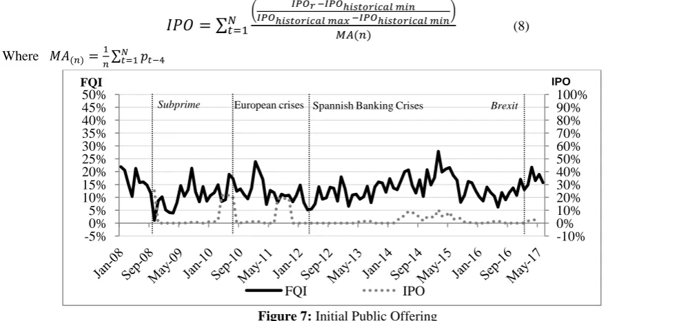
4.7 IPO / ISO
The ability to channel savings into productive investment is synonymous of the degree of financial market development. A large part of the theoretical literature has shown that both the Initial Public Offering (IPO) and the Initial Selling Offering (ISO) show greater visibility for the manufacturing sector. Mehran and Peristiani (2009); Bharath and Dittmar (2010); and Cao, Gustafson, and Velthuis (2017) show that institutional ownership, visibility and liquidity in companies that make the leap to financial markets increase simultaneously.
All of this reflects the fact that the most active markets in terms of IPOs have been further developed. Funds have been quantified at both the IPO and ISO levels and operations in which the share capital does not change, but rather a transfer of ownership of all or part of the shares (ISO) have been quantified, as well as the operations for which a company offers newly issued shares, as a result of a capital increase (ISO). In order to do this, standardization has been developed in the same way as volume and capitalization. The elaboration has been introduced a moving average of four months that calculates the capital inflows allowing in a more reliable way to smooth the inflows, observing the true market trend.
(8) Where
Figure 7: Initial Public Offering
The Spanish market, despite the economic crisis, has been a good reference in showing a good capacity to generate capital. However, the graph shows a turning point in the Spanish banking crisis. Since the end of September 2012, there has been a
-10% 0% 10% 20% 30% 40% 50% 60% 70% 80% 90% 100% -5% 0% 5% 10% 15% 20% 25% 30% 35% 40% 45% 50%
FQI Volatility
FQI Volatility
Brexit Subprime European crises Spannish Banking Crises
-10% 0% 10% 20% 30% 40% 50% 60% 70% 80% 90% 100% -5% 0% 5% 10% 15% 20% 25% 30% 35% 40% 45% 50%
FQI IPO
FQI IPO
1416
Damià Rey Miró
1, AFMJ Volume 3 Issue 03 March 2018
higher activity in line with the growth of the Spanish economy. In this sense, the IPO market in Spain in the first six months of 2017 was the market with the largest capacity to generate capital in the EMEA region (Europe, Middle East, India and Africa).
4.8 Capital Expansions
Finally, financial operations have been quantified in order to increase the equity of the different listed companies. In regards to capital increases, it was intended to reflect only the ability of companies to raise capital. In view of this, the authors did not want to study the reasons for the extensions, neither the costs that the entity experiences nor the repercussion that exists within the entity itself. Works such as Pastor and Martin (2004) already detected in the Spanish capital market a significant decline in the profitability of the securities of those companies that have increased capital through the issuance of new shares. Thus, it is a phenomenon that has been contrasted in other markets as show the works of Kang, Kim and Stulz (1999) in Japan; Jeanneret (2000) in the French market; and Stehle, Ehrhardt and Przyborowsky (2000) in Germany.
However, it has not been analyzed whether there has been a contribution of funds by the shareholders or whether it has been made from reserves or profits. What has been emphasized is the ability of the market to capture resources. In doing so, the formulation shows the relationship between the capital increases and the admitted capital, taking into account the share premium and showing a quarterly moving average (just like the ISO variable) in order to observe the market trend.
(9)
Where
Figure 8: Capital Expansions
The increased evolution of capital in the Spanish market has been continuous, being an essential engine for the financing of the listed companies. The evolution of this type of operations has experienced a clear upward trend within the quotations motivated by two great reasons; the first, the ease of financing that have been quoted because of the sharp decline in interest rates; and the second, the progressive increase in the importance of transactions related to shareholder remuneration of the type of scrip dividend7.
A pattern has been observed in the computation of the flows, where a certain concentration is detected in the central months of the year. Likewise, no significant correlation coefficient is detected with any of the variables described.
4.9 Model Aggregation
As a whole, the aggregate model provides a value that describes all the parameters of the subscripts discussed in the previous chapter. The Financial Quality Index (FQI) is a synoptic measure that shows the average progress achieved by a market in eight basic dimensions (see the aggregated index formula in the Appendix).
As indicated at the beginning of the section and due to the relevance of all the variables, the development of the formula implies the identical weighting of the eight dimensions, all in order to show with maximum objectivity the environment in which the financial flows. In four of the eight dimensions present in the formulation, the historical limits corresponding to the range of data available for the study are used in the calculation, which can lead to problems in comparison with other markets.
7
The dividend in shares (scrip dividends or scrip issue) is a form of remuneration to shareholders through the free delivery of new shares of the same entity.
-10% 0% 10% 20% 30% 40% 50% 60% 70% 80% 90% 100%
-5% 0% 5% 10% 15% 20% 25% 30% 35% 40% 45% 50%
FQI Capital expansion
FQI Capital expansions
1417
Damià Rey Miró
1, AFMJ Volume 3 Issue 03 March 2018
However, based on the references provided by the FESE (Federation of European Securities Exchanges) on international markets, future work can establish differentiated levels of quality and scales according to the historical references of each market segment. Also, another drawback derived from the formulation is the change that may occur in the limits used, since this involves changes in the historical FQI.
Even so, the authors consider that this is not a problem since it serves as a sample of the changing and adaptive reality of the concept of "market quality". Regarding itself, the IBEX 35, chosen as a reference for the formulation, also has a composition that changes over time and has an impact on its evolution. However, when changes are approved by the Technical Advisory Committee of the index, the FQI also adapts them reflecting a reliable image of reality.
5. Econometric evaluation and analysis of the FQI financial quality index
5.1 Robustness analysis of the FQI financial quality indicator
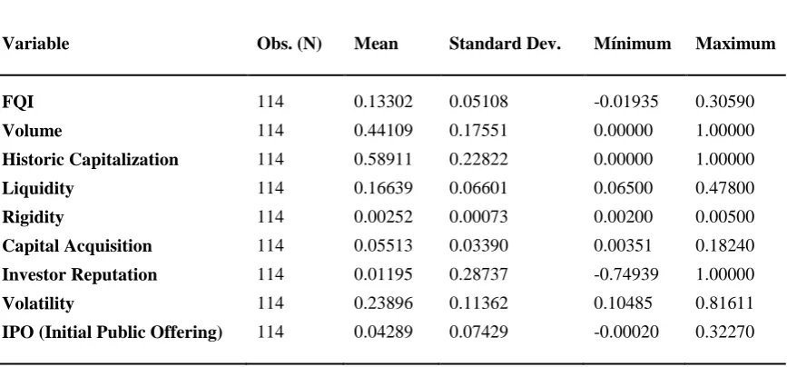
Although the variables that have been chosen for the construction of this financial quality index (FQI) considering the empirical evidence on the financial markets and the factors that affect that market, it is necessary to perform the statistical tests and econometric variables in order to evaluate the robustness of the indicator, as well as its limitations. Table 1 summarizes the descriptive statistics of the model variables.
Table 1: Summary of FQI Variables
Variable Obs. (N) Mean Standard Dev. Mínimum Maximum
FQI 114 0.13302 0.05108 -0.01935 0.30590
Volume 114 0.44109 0.17551 0.00000 1.00000
Historic Capitalization 114 0.58911 0.22822 0.00000 1.00000
Liquidity 114 0.16639 0.06601 0.06500 0.47800
Rigidity 114 0.00252 0.00073 0.00200 0.00500
Capital Acquisition 114 0.05513 0.03390 0.00351 0.18240
Investor Reputation 114 0.01195 0.28737 -0.74939 1.00000
Volatility 114 0.23896 0.11362 0.10485 0.81611
IPO (Initial Public Offering) 114 0.04289 0.07429 -0.00020 0.32270
Multicollinearity: Among the factors to be evaluated and due to the number of variables that make up the FQI index, the presence of multicollinearity, defined as the presence of a strong correlation between explanatory variables, is a factor that can affect the index performance.
The statistic that allows evaluating the existence of multicollinearity for a set of explanatory variables is the VIF (Variation Inflation Factor). In a multiple regression model, there is a serious problem of multicollinearity when the VIF of some coefficient is higher or the average of the set of explanatory variables or regressors is 10 or more. For the case of FQI, this value is 2.35, which allows us to discard the existence of multicollinearity. Consequently, performing a principal component analysis to reduce the number of factors or variables that make up the index is not necessary for the case of the FQI, so we can conclude that its eight variables or components are necessary.
Table 2: Statistics Tests FQI Model
VARIABLES FQI
Volume 0.125***
(-0.000066)
Historic Capitalization 0.125***
(-0.000023)
1418
Damià Rey Miró
1, AFMJ Volume 3 Issue 03 March 2018
(-0.00018)
Rigidity -0.0616***
(-0.01160)
Capital Acquisition 0.124***
(-0.000205)
Investor Reputation 0.125***
(-0.000026)
Volatility -0.125***
(-0.000081)
IPO (Initial Public Offering) 0.125***
(-0.000107)
Observations 114
R-squared 1.00
Variance Inflation Factor (VIF) 2.35
Durbin-Watson d-statistic (Autocorrelation) 1.9337
Breusch-Pagan / Cook-Weisberg (Heteroskedasticidad) 0.4063
Ramsey (Omitted Variables) 0.3868
Standard error in parenthesis *** p<0.01, ** p<0.05, * p<0.1
According to the results of Table 2, it is concluded that both the variables and the general model approve the rigorous statistical and econometric tests. Based on these results we proceed with the following levels of robustness of the model. As can be seen, the tests reject the presence of autocorrelation (Durbin-Watson test), heteroskedasticity (Breusch-Pagan/Cook-Weisberg test) and absence of relevant variables in the model (Ramsey test).
Unit root: For an OLS estimation to be valid, the error term of the equation must be invariant over time or stationary. On the other hand, a non-stationary series, meaning data series with a time variance component follows the form
(10)
In the equation, is a random perturbation with zero mean and constant variance. In this model, if then is a non-stationary random walk with the form . The latter equation is said to have a unit or integrated root of order one [I
(1)] because the coefficient rho is equal to unity. Because the total value of the previous period is moved to the current period, the values of the disturbance never fade. The continuous accumulation of errors creates the problem that a non-stationary series will tend towards an infinite variance.
Table 3 summarizes the results of the application of eleven unit root tests for FQI. The tests correspond to the traditional Dickey-Fuller ADF test (Augmented Dickey and Dickey-Fuller 1979), the PP test (Phillips and Perron 1988) and the KPSS test that takes stationarity as a null hypothesis (Kwiatkowski, Phillips, Schmidt and Shin 1992).
From all these tests the KPSS proposal is the most powerful and should be the last word in the unit root test since this test has better properties in small samples among all the unit root tests (Metes 2005). Specifically, the KPSS test specifying that the auto covariance function should be weighted by the quadratic Spectral Kernel rather than the Bartlett Kernel and with the specification that the automatic bandwidth selection procedure proposed by Newey and West (Newey and West 1994) as described by Hobijn in his publication (Hobijn et al., 1998, 7), is the one to be used to determine the maximum number of lags, which for the case of FQI is three (3), providing the optimum bandwidth for the proof.
Table 3: Unit Root Tests
Unit Root Test FQI
Dickey-Fuller (DF-GLS) UR
1419
Damià Rey Miró
1, AFMJ Volume 3 Issue 03 March 2018
Phillips-Perron (rho) No UR
Phillips-Perron (tau) No UR
KPSS (level) No UR
KPSS (tendency) No UR
KPSS (auto) No UR
Concluding, Table 3 shows that although the Dickey-Fuller test fails to reject the null hypothesis that confirms the presence of a unit root in the FQI series, the KPSS results are robust, finding no statistical evidence to reject the hypothesis that the series is stationary. The above results suggest that the FQI series is stationary and therefore apt to be analyzed with more advanced time series methods.
Changes in the smoothing parameter: In order to decrease or eliminate the influence of random variations, an exponential weighted moving average is used with a given value for the smoothing parameter defined as lambda (λ). Thus, a large value of λ gives more weight to recent data and less weight to the old data and exactly the opposite for small values of λ.
Figure 9: Changes Smoothing Parameter (λ)
Monthly data from January 2008 to June 2017 (N=114)
Consequently, for these three lambda values Figure 9 illustrates small, almost insignificant differences between the new indicators, so it can be concluded that changes in the smoothing parameter do not imply any relevant alteration in the general behavior of the indicator
Following the logic of Holló, Kremer and Lo Duca (2012), the decay factor or smoothing parameter using lambda level equal to 0.93 represents an intermediate value. Under the same logic, other extreme values for the lambda factor have been estimated for the FQI as 0.98, considered a high value, and a value of 0.88, considered as a low value, to determine the behavior of the index against more extreme values. The path for the three lambda values (λ) is shown in Figure 9.
1420
Damià Rey Miró
1, AFMJ Volume 3 Issue 03 March 2018
Figure 10: FQI ForecastMonthly data from January 2008 to June 2017 (N=114)
5.2 Ability to identify periods of different financial quality
Important as robustness is, also the ability of the FQI to identify episodes of changes in quality in the past. Theoretically, a financial quality indicator such as the FQI decreases considerably under an event that can generate systemic risk and reach unusually lower levels in comparison to events where financial risks at the systemic level are absent.
In this study and for the FQI indicator, the high-stress events will result in falls in the FQI indicator (quality reduction). Following this line of analysis, Figure 10 illustrates the minimum and maximum points reached by the indicator. The minimum point occurs in October 2008 that marks the collapse of Lehman Brothers and the rescue of AIG, as well as the beginning of the Great Recession as a result of the subprime crisis unleashed in the United States that then spread out to the rest of financial markets. The low level of the indicator remained for several months due to the transmission mechanism of that contagion to the real economy. Then, the FQI starts a rebound to average levels of quality. This phase is shown on the first vertical line of the FQI evolution chart.
Figure 11: FQI Evolution
Monthly data from January 2008 to June 2017 (N=114)
1421
Damià Rey Miró
1, AFMJ Volume 3 Issue 03 March 2018
expelled from the Euro-zone by failing the International Monetary Fund guidelines, a new bailout was agreed for the country, which also brought some peace of mind to the financial global markets.
Subsequent to these events, the FQI begins a decline until August of 2015. The reason for these decreases was mainly due to the weakness of the European financial sector due to the low yields of the sector. Around 2 billion of Euros in the Euro-zone sovereign bonds, one-third of the total outstanding, were traded in 2015 with negative returns. Finally, the fall in the FQI is accentuated during the second half of 2016 as a result of the Brexit event; however, this event does not have a notable impact on the financial markets, showing a strong recovery afterward.
5.3 Regions and boundaries
Another characteristic required for a financial quality index is the ability to react to losses and increases in the financial market, which becomes a tool for financial market players from the investors themselves to those who are in charge of supervising, developing and evaluating policies in the financial industry.
A first approximation may be the rule of imposing a limit of one standard deviation below or above the average as the limit to classify the event as a loss or increase in severe quality, but this rule makes the FQI to be classified as an index with normal distribution, which in the vast majority of cases is somewhat implausible given the nature of financial and macroeconomic data whose third and fourth moments (symmetry and kurtosis, respectively), deviate from the statisticians representing a normal distribution (Caldarelli, Elekdag and Lall 2009). Notwithstanding the above, the FQI proposed in this study passes the normality tests of Shapiro-Wilk and Shapiro-France.
Even so, the authors believe necessary to use a more rigorous and sophisticated classification methodology from the econometric point of view. The models that meet this requirement are the so-called Markov-Switching models, which are able to capture the dynamics of financial quality by assuming that the properties of the FQI, as a time series, are state-dependent. Also, it is important that the time series (FQI) be a stationary series, as tested in the unit root section of the robustness analysis above-discussed.
Thus, a convenient and adequate assumption about the unobserved state is that it follows a Markov chain and it is for this reason that the region-change or regime-switching models are known as Markov-Switching models. Initially, these models were developed by Quandt (1972), Goldfeld and Quandt (1973) and later extended to autoregressive (AR) and nonlinear processes by Hamilton (1989).
For FQI, the estimated coefficients in a Markov-Switching model are represented as the general equation
+ for the states (11)
Table 4 summarizes five specifications of Markov Switching models, each of which represents the general equation of the model.
Table 4: Markov-Switching Models
Model Log-Likelihood AIC1 BIC2 HQIC3 D-Watson
DR2 192.945 -375.89 -362.21 -3.25 1.51
DR2V 193.551 -375.10 -358.68 -3.23 1.49
DR3 195.720 -371.44 -344.08 -3.16 1.60
AR211 195.233 -376.47 -357.37 -3.26 2.48
AR212 193.427 -368.85 -344.39 -3.20 2.67
Monthly data from January 2008 to June 2017 (N=114)
1BIC: Bayesian information criterion 2AIC: Akaike information criterion
3HQIC: Hannan–Quinn information criterion
1422
Damià Rey Miró
1, AFMJ Volume 3 Issue 03 March 2018
According to the results, the model that best represents the dynamics of the data, according to the statisticians in Table 4, is the DR2 model which is a dynamic model with one lag for FQI ( ) and two states of rapid adjustment and variation of
coefficients, but in which the standard deviation (σ) of the model remains constant. In contrast, the DR2V model is similar to the DR2 model but where variance is allowed to vary.
However, this second model is less optimal than DR2 and that in the opinion of the authors is due to the short history of the index and its lower exposure to stressful events. The authors consider that with three or more years of history and data, it is very likely that the optimal model will be closer to a model of the DRV2 type, in which all coefficients vary including the standard deviation.
Table 5: Transition Probabilities
Prob. Transición Estimado Error Estd. [95% Intervalo Conf.]
p11 0.944142 0.029795 0.848149 0.980825
p12 0.055858 0.029795 0.019175 0.151851
p21 0.096590 0.064207 0.024654 0.311409
p22 0.903410 0.064207 0.688591 0.975346
Table 6: Expected Event Duration
Expected Duration Estimated Std. Error [95% Conf. Interval]
Stage 1 17.90255 9.549316 6.585405 52.15047
Stage 2 10.35302 6.882023 3.211215 40.56148
It is noteworthy that although the Durbin-Watson statistic for serial autocorrelation is not perfect or close to the value 2.0, it is within the normal ranges of variation between 1.5 and 2.5 (Durbin, J. and Watson, GS 1951).
The most relevant of these results is that the DR2 model clearly identifies two different states for the FQI, which were already analyzed on the basis of Figure 10. Based on the selected model, we proceed to estimate the transition and duration of the states. Tables 5 and 6 summarize these results.
Relevant information can be extracted from Tables 5 and 6. In fact and according to the transition probabilities of Table 5, which clearly identifies two different states for the FQI, the P11 value of 0.944 indicates the probability of remaining in state 1, and this probability is very high or highly persistent (near the unit or value 1). On the other hand, the P12 value of 0.056 indicates that the probability of transit from state 2 to state 1 is low. Finally, the value P22 tells us that once the FQI reaches state 2, its probability of remaining in this state is high and persistent (0.903). In other words, once FQI arrives at state 2, a strong fiscal, monetary or macroeconomic policy is required so that the execution of that policy allows the FQI to be transited from state 2 to initial state 1.
Complementarily, Table 6 indicates that for FQI the estimated duration of staying in state 1, which was identified as the 2008 subprime crisis with all its collateral events and in which the FQI reached its minimum, is close at 18 months while the second state identified by its maximum value, which is in February 2015, reaches a duration of just over 10 months, or almost throughout the entire year 2015.
Finally and in relation to the ability of the FQI indicator, it is of interest to determine the regions and limits for which the FQI is sensitive to different shocks and events in both the financial market and the real economy. Following a Threshold-Regression model will be estimated, that unlike the Markov-Switching models assumes that the transitions between states of a variable, FQI in this study, are triggered by observable variables that at some point of time cross certain limits and these limits must be estimated or determined.
1423
Damià Rey Miró
1, AFMJ Volume 3 Issue 03 March 2018
Formally, consider a Threshold Regression with two regions defined by a threshold γ as
(12) (13)
Where , is the dependent variable, is a vector of dimension 1xK of covariates possibly containing lagged values of , β is a vector Kx1 of invariant parameters region, is an error with mean 0 and variance , is a vector of exogenous variables with vectors of region-specific coefficients y , and is a threshold variable that can also be one of the variables in or .
The parameters of interest are, and . Region 1 is defined as the subset of observations whose value of is less than the threshold. Similarly, Region 2 is defined as the subset of observations in which the value of is greater than the threshold. Inference about the gamma parameter is complicated because of its non-standard asymptotic distribution (see Hansen 1997, 2000).
A threshold regression uses conditional least squares to estimate the regression model parameters. Structuring a model for the FQI, its lag value and the variable industrial production are estimated five models with one and two lags, of which there are two competing models, the first with one lag and the second with two lags for the FQI. Of the two models selected, the model with one lag is the model of choice considering the information criteria already above-described. The values for the selection criteria of both models are shown in Table 7.
Table 7: Threshold Model Results
Model T1 T2 AIC BIC HQIC SSR*
Single Lag Model 0.1090 - -721.353 -704.988 -714.712 .1716
Two Lags Model 0.1267 0.1487 -720.493 -695.946 -710.532 .1640
Monthly data from January 2008 to June 2017 (N=114) *SSR: Sum of Squared Residuals
From the results of Table 7, it can be inferred, according to the information criteria AIC, BIC, and HQIC, that the model of one lag is the model to be selected. Basically, the model imposes a single limit whose value is 0.1090 that divides the series into two regions; one of low quality for values less than or equal to 0.1090 and another of high quality for values higher than 0.1090. Figure 12 shows these two regions derived from the threshold model.
Figure 12: FQI – Changes in Financial Quality
Monthly data from January 2008 to June 2017 (N=114)
5.4 Effects of the real economy and the stress index (FMSI) on the FQI
1424
Damià Rey Miró
1, AFMJ Volume 3 Issue 03 March 2018
The results of the VAR model conclude that the manufacturing PMI is significant at a significance level of 1%, in addition to concluding that to some extent, the manufacturing PMI determines the trajectory of the FQI. Indeed and based on the Granger test, there is a causal relationship from the manufacturing PMI to the FQI, and this relationship is unidirectional, that is, it is not possible to determine a cause-effect relationship in the opposite direction or from FQI to the PMI index. .
Notwithstanding the above, this causal relationship seems to be stronger in the region of low quality, in which the FQI indicator is below the threshold established in the previous section of 0.1090. It is in that region in which the FQI and the growth of the manufacturing PMI follow a very close trajectory. For values above the threshold (values greater than 0.1090), the relationship or trajectory of both indicators becomes more divergent, which is consistent with values of the manufacturing PMI higher than the value of 50, which is the threshold value established for this index. The graph below shows this change in the relationship between the two indicators as it moves from a low-quality region (left side of the chart) to a high-quality region (right region of the chart), specifically starting in 2014.
Figure 13: FQI – Manufacturing PMI
Monthly data from January 2008 to June 2017 (N=114)
As regards the effect of market stress on the FQI, it is determined that there is a negative and significant correlation at the level of 1% of -0,495 between both indices. Using the same econometric approach (VAR), it is concluded that the stress index for the Spanish financial market FMSI (Financial Market Stress Index) of Estévez and Cambón, determines the trajectory of the FQI and this relationship is significant at the 1% level. Indeed and based on the Granger test, there is a causal and unidirectional relationship that goes from the FMSI to the FQI. In other words, high levels of stress in the financial market decrease the quality of the market, a result that is consistent with what the authors expected. Figure 14 depicts the inverse movement between both indices; the indexes diverge in periods of high stress and coincide with periods of low stress in the financial market, an indicator of its quality.
Figure 14: FQI - FMSI (Financial Market Stress Index)
Monthly data from January 2008 to June 2017 (N=114)
1425
Damià Rey Miró
1, AFMJ Volume 3 Issue 03 March 2018
The quality of a financial market is a heterogeneous concept due to the multiple dimensions that characterize it. However, in this research work, the authors have been able to agglutinate the most important characteristics of a particular market such as the Spanish stock market. Looking in perspective at the changes of the different indicators over time and analyzing them in turn as a whole, can provide a more objective sample for the investor and for the companies in order to evaluate the quality of the market.
The FQI financial quality indicator developed in this research provides valuable information both to investors and companies about the proper functioning of a market. An FQI higher than 0.1090, that is, of high market quality, is reflected in a probability of positive return close to 70% for the IBEX 35 in the same month. Likewise, when the FQI is located in high-quality market environments, there is also an improvement in the capture of capital by companies. In addition, the FQI reflects and predicts to a large extent the moments of greatest tension due to periods of stress such as financial crises, as well as the economic recovery of the Spanish economy. Particularly in Spain, there is a great symmetry between the development of the stock market and the country's economic growth (GDP).
The study also allows extracting or inferring that market fragmentation has a significant impact on the depth and liquidity of the market. Obviously, the development of alternative trading platforms can mean that in situations of market stress, investors have problems transforming the asset into liquidity. In this sense and as it has been widely explained in the financial literature, markets tend to contagion and overreaction of assets that can lead to liquidity problems in the financial system itself. The FQI shows us in the studied period that includes from the year 2008 until the end of June 2017, there is an estimated time of permanence for the FQI above the high quality zone, that is, the FQI remains above the threshold 0.1009 62.28% of the time for the period elapsed between 2008-2017, a true reflection of the high level of development of the Spanish market and given the level of turbulence present in global markets.
On the other hand, the FQI shows a high degree of inverse correlation with the market stress index (FMSI). Indeed, if we observe the periods of greatest stress in the Spanish market, the US subprime crisis (October 2008) and doubts about the soundness of the Spanish financial sector (March 2013), the financial quality index shows an absolute minimum and a relative minimum that it coincides with the absolute maximum of market stress and a relative maximum in the FMSI. Therefore, it is corroborated that the market stress events are reflected in periods of low quality, as evidenced by the VAR analysis between both variables developed in this study and confirming the existence of a cause-effect relationship between FQI and FMSI. However, both periods of stress and those of low quality are rather punctual periods, but they tend to have replicas with relative minimums/maximums above the minimum / maximum established prior to the stress period.
Finally, and based on the results of a second VAR model, the manufacturing PMI has a direct causal relationship (causality of the Granger type) over the FQI, especially when the economy faces scenarios of low financial quality. In other words, falls in the manufacturing PMI below its threshold of 50 points are not only an indication that the real economy may be entering a period of deceleration or recession but also a period of low quality in the financial market.
Consequently, the FQI is an indicator capable of capturing the effect of the real economy on the quality of the market in its real dimension, making it, in the opinion of the authors, an indicator of relevance not only for the qualitative diagnosis of the financial market based on measurable and well-founded variables, but also regarding the possible corrections that may be in the making on the Spanish financial market.
7. References
1. Akerlof, George A. (1970). "The Market for 'Lemons': Quality Uncertainty and the Market Mechanism." Quarterly Journal of Economics, 84(3), pp. 488-500, 1970.
2. Acharya, V. V., Pedersen, L. H., Philippon, T. and M. Richardson (2010). “Measuring Systemic Risk”. FRB of Cleveland Working Paper No. 10-02.
3. Adrian, T. and M. K. Brunnermeier (2011). “CoVar”. NBER Working Paper No. 17454.
4. Beck, T., A. emirg -Kunt, and R. Levine. 2010. “Financial Institutions and Markets Across Countries and over Time: The Updated Financial evelopment and Structure atabase.” World Economic Review 24(1):77–92.
5. Bharath, Sreedhar & Dittmar (2010). Amy. Why do firms use private equity to opt out of public markets?. Review of Financial Studies. Published - May 2010
6. Brownlees, C. T. and R. Engle (2012). “Volatility, Correlation and Tails for Systemic Risk Measurement”. Working Paper, NYU.
7. Caldarelli, R., Elekdag, S. A. and S. Lall (2009). “Financial Stress, ownturns, and Recoveries”. International Monetary Fund, Working Paper WP/09/100.
1426
Damià Rey Miró
1, AFMJ Volume 3 Issue 03 March 2018
9. Caporin, M., Pelizzon, L., Ravazzolo, F. and R. Rigobon (2013). “Measuring Sovereign Contagion in Europe”. NBER Working Paper No. 18741.
10. Dambra, Michael and Gustafson, Matthew and Pisciotta, Kevin J, Post-IPO Market Returns and the Benefits to Going Public (June 8, 2017)
11. Dickey, D. A., and W. A. Fuller (1979). Distribution of the estimators for autoregressive time series with a unit root. Journal of the American Statistical Association 74: 427–431.
12. iebold, F. X. and K. Yilmaz (2009). “Measuring Financial Asset Return and Volatility Spillovers, with Application to Global Equity Markets”. The Economic Journal, Vol.119 (534), pp. 158–171.
13. Drewnowski, Jan & Scott, Wolf (1966). The level of living index, United Nations Research Institute for Social Development, Geneva
14. Durbin, J., and G. S. Watson (1950). Testing for serial correlation in least squares regression. I. Biometrika 37:409–428. 15. Durbin, J., and G. S. Watson (1951). Testing for serial correlation in least squares regression. II. Biometrika. 1951 Jun;
38(1-2):159-78.
16. Estévez Leticia and Mª Isabel Cambón (2015). A Spanish Financial Market Stress Index (FMSI). Research, Statistics and Publications Department, CNMV.
17. Eugene F. Fama (1965). “The Behavior of Stock Market Prices," The Journal of Business, vol. 38, no. 1. (1965): 34-105.
18. Fama, E. (1965). “The behavior of stock-market prices”. The Journal of Business 38, 34–105.
19. Forbes, K. and R. Rigobon (2001). “Measuring Contagion: Conceptual and Empirical Issues”. International Financial Contagion, Chapter 3, pp.43-66.
20. Goldfeld, S. M., and R. E. Quandt. (1973). A Markov model for switching regressions. Journal of Econometrics 1:3–15. 21. Goldsmith, Raymond W. (1969). Financial structure and development. New Haven, CT: Yale University Press.
22. Gray, . F. and A. A. Jobst (2011). “Modelling systemic financial sector and sovereign risk”. Sveriges Riksbank Economic Review, 2011:2, pp.68-93.
23. Hamid Mehran and Stavros Peristiani (2009). Financial Visibility and the Decision to Go Private Federal Reserve Bank of New York Staff Reports, no. 376 June 2009
24. Hamilton, J. . and R. Susmel (1994). “Autoregressive conditional heteroskedasticity and changes in regime”. Journal of Econometrics, No. 64, pp.307-333.
25. Hansen, Bruce E. (2000). "Testing for structural change in conditional models," Journal of Econometrics, Elsevier, vol. 97(1), pages 93-115, July.
26. Hansen, Bruce E. (1997). "Threshold effects in non-dynamic panels: Estimation, testing and inference," Boston College Working Papers in Economics 365, Boston College Department of Economics.
27. Hobijn, B., P. H. Franses, and M. Ooms (1998). Generalizations of the KPSS-test for stationarity. Econometric Institute Report 9802/A, Econometric Institute, Erasmus University Rotterdam.
28. Holló, ., Kremer, M. and M. Lo uca (2012). “CISS-a composite indicator of systemic stress in the financial system”. European Central Bank, Macroprudential Research Network, Working Paper Series March 2012, No.1426.
29. Horvath, R., & Poldauf, P. (2012). International stock market comovements: what happened during the financial crisis? Global Economy Journal, 12(1).
30. Hovakimian, A., Kane, E. J. and L. Laeven (2012). “Variation in Systemic Risk at US Banks uring 1974-2010”. NBER Working Paper No. 18043.
31. Huang, X., Zhou, H. and H. Zhu (2011). “Systemic risk contributions”. Finance and Economics Discussion Series 2011-08, Board of Governors of the Federal Reserve System (US).
32. Hyde, S., Bredin, . and N. Nguyen (2007). “Correlation dynamics between Asia-Pacific, EU and US stock returns”. International Finance Review, Vol. 8, Chapter 3, pp. 39-61.
33. Illing, M. and Y. Liu (2006). “Measuring financial stress in a developed country: An application to Canada”. Journal of Financial Stability, Vol. 2, No. 4, pp. 243-265.
34. IMF-BIS-FBS (2009): “Guidance to Assess the Systemic Importance of Financial Institutions, Markets and Instruments: Initial Considerations”. International Monetary Fund, Bank for International Settlements and Financial Stability Board. 35. Dubois, Michel and Jeanneret, Pierre (2000). The Long-run Performance of Seasoned Equity Offerings with Rights:
Evidence from the Swiss Market (January 2000).
36. Kang, J.K., Y.C. Kim, and R.M. Stulz. (1999) “The Underreaction Hypothesis And The New Issue Puzzle: Evidence From Japan.” Review of Financial Studies, Vol. 12, pp. 519-534