On the Performance of Haar Wavelet Approach for Boundary Value Problems and Systems of Fredholm Integral Equations

http://www.sciencepublishinggroup.com/j/mcs doi: 10.11648/j.mcs.20170204.12

On the Performance of Haar Wavelet Approach for

Boundary Value Problems and Systems of Fredholm

Integral Equations

I. K. Youssef

1

, R. A. Ibrahim

2

1

Department of Mathematics, Ain Shams University, Cairo, Egypt 2

Department of Mathematics and Engineering Physics, Faculty of Engineering_Shoubra, Benha University, Cairo, Egypt

Email address:

[email protected] (I. K. Youssef), [email protected] (R. A. Ibrahim)

To cite this article:

I. K. Youssef, R. A. Ibrahim. On the Performance of Haar Wavelet Approach for Boundary Value Problems and Systems of Fredholm Integral Equations. Mathematics and Computer Science. Vol. 2, No. 4, 2017, pp. 39-46. doi: 10.11648/j.mcs.20170204.12

Received: May 31, 2017; Accepted: June 13, 2017; Published: July 17, 2017

Abstract:

The Haar wavelet method applied to different kinds of integral equations (Fredholm integral equation, integro-differential equations and system of linear Fredholm integral equations) and boundary value problems (BVP) representation of integral equations. Three test problems whose exact solutions are known were considered to measure the performance of Haar wavelet. The calculations show that solving the problem as integral equation is more accurate than solving it as differential equation. Also the calculations show the efficiency of Haar wavelet in case of F. I. E. S and integro-differential equations comparing with other methods, especially when we increase the number of collocation points. All calculations are done by the Computer Algebra Facilities included in Mathematica 10.2.

Keywords:

Integral Equations, Haar Wavelets, BVP, System of Integral Equations, Collocation Method

1. Introduction

Many applications in scientific fields such as physical and engineering problems can be formulated as integral equations or as differential equations. Differential equations can be reformulated in the form of integral equations while not every integral equations can be differentiated to obtain a corresponding differential equation, equivalence requires restricted regularity conditions on the kernels [1, 2]. The problems which can be formulated as integral and differential equations are introduced. The analytical solution has its difficulties which gives the chance to numerical analysis to appear, especially with the huge development in programming and computer systems. The last step in the numerical treatment is the solution of the algebraic system of the mathematical

model [3]. Recently a great deal of interest has been focused on the solution of integral and differential equations by the wavelet methods, the first paper which used Haar wavelet method to solve integral equation has presented in 1991. The basic idea of Haar wavelet method is to convert the differential and integral equations into a system of algebraic equations. In this paper we use the Haar wavelet method to solve BVP and its integral representation. We consider the relation between the numerical treatments of the two point BVP, [3, 4]

+ = ; ≤ ≤ ,

= , = (1)

And its equivalent second kind Fredholm integral representation

= + − + , − , ; (2)

where the kernel , is defined as

We consider also the integro-differential equation

+ ! = , "# + $ % + ; = & (4)

A system of linear Fredholm integral equation which appears in many applications in physics and engineering is considered. The linear system of Fredholm integral equations takes the form, [5, 6]

' = ' + ∑+), _* ') , )

- = 1,2, … , 1 2 (5)

Where _'∈ 45"0,1%, _')∈ 45 "0,1% × "0,1% for -, 8 =

1,2, … , 1 and _'are unknown functions. The system (5) can be written in matrix form as

9 = : + ; , 9_* (6)

Where 9 = < 5

⋮

+

> , : = < 5

⋮

+

>,

; , = <

, 5 , … + ,

5 , 55 , … 5+ ,

⋮ ⋮ … ⋮

+ , +5 , … ++ ,

>

2. Haar Wavelet Functions and Its

Integration

The idea of Wavelet analysis is that it represents a function in terms of a set of basic functions, called wavelets, constructed from transformation and dilation of mother wavelet. The wavelet function takes the form

?@,A = 2@ 5⁄ ? 2@ − , C = 0,1, … ; 0 ≤ < 2@, 0 ≤ < 1 (7)

The wavelet basis satisfy the following properties a) The orthogonality property

E ?F ?@

* = 1 ; G = C0 ; G ≠ C

b) Most of the functions have a small interval of support [7-11].

Definition: Let ∈ 45 I for 1 ∈ J, K₊: 45 I → 45 I be given by K₊ = − 1 and N: 45 I → 45 I be given by N = √2 2 operators K₊ and N are called translation and dilation operator.

There are many types of wavelet functions; one of them is the Haar functions, which are mathematically the simplest wavelets. The orthogonal set of Haar functions is defined as a group of square waves with magnitude of ±1 in some intervals and zero elsewhere. They are step functions (piecewise constant functions). Haar transform or Haar wavelet transform has been used as an earliest example for orthonormal wavelet transform with compact support

The Haar wavelet family are given as, [6-9]

ℎF = R

1 S- ∈ " , % −1 S- ∈ " , T%

0 UV8UWℎU-U

(8)

The notations =_XA, =AY*.Z_X T =AY_X are introduced. The integer [ = 2@, C = 0,1,2, … , \ indicates the level of wavelet (dilation parameter); = 0,1,2, … , [ − 1 is the translation parameter. The integer \ determines the maximal level of resolution, the index G obtained from the relation

G = [ + + 1 which has minimum value G = 2 [ =

1, = 0 , which called the mother function, and maximum value G = 2] where ] = 2^. the index G = 1 corresponds to the scaling function

ℎ = _1 S- 0 ≤ < 1_{0 UV8UWℎU-U}

The following notations are introduced, [9, 10]

`F = ℎ<sub>*</sub>a F ; bF = `_*a F (9)

For the scaling function we have

` = ; S- 0 ≤ < 1_{0; UV8UWℎU-U ; b} = R

5

2 ; S- 0 ≤ < 1 0 ; UV8UWℎU-U

Else

`F = R

− S- ∈ " , % T − S- ∈ " , T%

0 UV8UWℎU-U

bF =

c d e d

f a5 g S- ∈ " , %

g_{Y h}g _{h a}g

5 S- ∈ " , %

g_{Y h}g

5 S- ∈ " , %

0 UV8UWℎU-U

(10)

To discretize the functions ℎ_F we divide the interval

∈ "0,1% into 2] parts of equal length ∆ =_5j. Let us introduce the collocation points

k= k *.Z_5j ,

V = 1,2, … ,2]2 (11)

Any function , ∈ "0,1% can be written as

Where _F are the Haar coefficients which can be determined by multiplying (12) by ℎ_X and integrating from 0 → 1 we get

E ℎX

* = Fn E ℎ* X ℎF 5j

F,

from the orthogonality condition

ℎX ℎF

* = 2

@_{; G G = [}

0; G G ≠ [ ⇒ F= 2@ _* ℎX

p (13)

The discrete form of eq. (12) at collocation points is

k = ∑5jF, FℎF k = ∑5jF, FqFk (14)

The matrix form of (14) is 9 = q where, 9 and are

2] row vectors and q = q_Fk = ℎ_{F k} is the coeffeficients matrix with dimension (2] × 2] [12-15].

3. Method of Solution

In this section we introduce how the Haar wavelet transform method can solve the BVP and its Fredholm integral form and the system of Fredholm integral equations.

3.1. Haar Solution of Second Order Two-Point BVP

The main advantage of the Haar wavelet method is its efficiency and simple applicability for a variety of boundary conditions [10,11,13]. Since the Haar wavelet is defined for the interval [0,1], then we transform the variable ∈ " , % in equation (1) into the variable ∈ "0,1% using

= _{− → if = , = 0 and if = , = 1}−

So equation (1) becomes

+ = ; 0 ≤ ≤ 1 ,

0 = , 1 = . （15）

In equation (15) let

= n FℎF 5j

F,

Integrating twice from 0 → , using the boundary conditions we get

= + 0 + n FbF 5j

F,

And

0 = − − n FwF 5j

F,

Where w_F= `_{* F} then can be written as

= + − + ∑5jF, F bF − wF (16)

Using (16) in (15) we get

n F"ℎF + bF − wF % 5j

F,

= + − −

Satisfying the previous equation at the collocation points (11) we obtain

∑5jF, F"ℎF k + "bF k − kwF%% = k + + − k− ,

V = 1, … ,2] (17)

Solving the linear system of algebraic (17) we obtain the unknowns _F, substituting in (16) we get the solution of the BVP [16,17].

3.2. Haar Solution of Fredholm Integral Equations

In equation (2) let

= ∑5jF, FℎF (18)

From (18) equation (2) becomes

∑5jF, FℎF − ∑5jF, FxF = ! (19)

Where

xF = , ℎF (20)

and

! = + − − , (21)

Satisfying equation (19) at the collocation points (11)

∑5jF, F"ℎF k − xF k % = ! k , V = 1,2, … ,2] (22)

Equation (22) is a linear system of algebraic equations in the unknowns _F, solving this system we obtain _F , substituting in (18) we solve the Fredholm integral equation (2) [9-11,18].

3.3. Haar Solution of Integro-Differential Equations

To solve the integro-differential equation (4), let

Where `_F = yℎ_F . Substituting from (23) in (4) we get

∑5jF, F"ℎF + ! `F − #IF − $xF %= −! + # z + (24) Where x_F given from (20) and

IF = , `F , z = ,

Satisfying equation (24) at the collocation points (11) to get the matrix form as

Α q + | − #I − $x = −&! + #&z + : (25) Where Α is a 2] vector of the coefficients _F ; (!, :, z) are 2] vectors and q = q_Fk= q_{F k} , I = I_Fk= I_{F k} ,

| = |Fk= ! k `F k [6,9,12].

3.4. Haar Solution of Linear System of Fredholm Integral Equations

Using equation (12) in equation (5) we obtain

∑5jF, 'FℎF − ∑5jF, 'FxF = : ; (26)

Where

: = < 5

⋮

+

>

xF

=

} ~ ~ ~ ~ ~ ~

•x = E ,

* ℎF … x+ = E* + , ℎF

x5 = E 5 ,

* ℎF … x5+ = E* 5+ , ℎF

⋮ ⋱ ⋮

x+ = E + ,

* ℎF … x++ = E* ++ , ℎF •

‚ ‚ ‚ ‚ ‚ ‚ ƒ

Satisfying equation (26) only at the collocation points (11) we get a linear system of algebraic equations

∑5jF, 'FℎF k − ∑5jF, 'FxF k = : k ,

V = 1,2, … ,2]; - = 1,2, … ,2] (27)

The matrix form of equation (27) is „… = : where

„ = †n F 5j

F,

n 5F 5j

F,

… n +F 5j

F,

‡,

: = <

k 5 k

⋮

+ k

> , … = <

q − x −x5 … −x+

−x 5 q − x55 … −x+5

⋮ ⋮ ⋱ ⋮

−x+ −x5+ … q − x++

>

Solving the linear system (27) we obtain _'F [6,9,12].

3.5. Haar Algorithm for Linear System of F. I. E.

a) Divide the interval [0, 1] into 2] part of equal length

∆ =_5j .

b) Compute the x matrix from the equation (26).

c) Solve the system (27) at the collocation points to determine _'F .

d) Substitute in (12), we get the solution of the system (5).

4. Numerical Examples

In this section some numerical examples are considered. The exact solution introduced to show the accuracy and efficiency of the used method. In the first example we compare between the second order two point BVP and its Fredholm integral representation. In the second example we solve a linear system of F. I. E. and compare our method with a domain decomposition method. In the third example, the solution of the integro-differential equation and comparing our solution with another method is introduced.

Example 1:

Consider the second order two point BVP, [3, 19]:

− + ˆ5 _{= 2 ˆ}5 _{‰G1 ˆ ,}

0 ≤ ≤ 1; 0 = 1 = 0. (28)

whose exact solution was given as

= sin ˆ . (29) The Fredholm integral form of equation (28) is

= 2 8G1 ˆ − ˆ5 y _{1 −}

* − ˆ5 y 1 − . (30)

It is an easy task to see that this integral equation (30) satisfies the boundary conditions in (28). Moreover the closed form solution (29) satisfies both the differential and the integral equation.

In equation (28) let

= n FℎF 5j

F,

Integrating twice from 0 → with boundary conditions we get on

‹ Œ = Œ‹ • + n FbF 5j

F,

0 = − n FwF 5j

F,

Where w_F defined before, then

= n FbF 5j

F,

− n FwF 5j

F,

Substituting in (28) we get

∑5jF, F"ˆ5bF − ˆ5 wF− ℎF %= 2ˆ5sin ˆ (31)

Satisfying equation (31) at the collocation points (11)

∑5jF, F"ˆ5bF k − ˆ5 kwF− ℎF k %= 2ˆ5sin ˆ k,

V = 1, … ,2] (32)

Solving the linear system (32) we determine _F. The solution of BVP (28), the exact solution and the error at different numbers of collocation points with different values of ] given in table 1.

Satisfying equation (30) at the collocation points (11)

k + ˆ5 _*yŽ 1 − k + ˆ5 _yŽ k 1 − = 2 8G1 ˆ k.

V = 1,2, … ,2] 2 (33)

putting = ∑5j_{F, F}ℎ_F , in equation (33) we have

∑F,5j F"ℎF k + ˆ5 1 − k _*yŽ ℎF + ˆ5 k _yŽ 1 − ℎF % = 2 8G1 ˆ k.

V = 1,2, … ,2] 2 (34)

For \ = 3 the solution of (30), the exact solution and the error between the exact solution and Haar solution are given in table 1.

Table 1. Comparison between Haar solution of BVP Ex. (1) and Haar solution of its Fredholm form with (J=3).

X / 32 Exact solution Haar (BVP) |‘’“”| Haar (F. I. E) |‘•.–.‘.|

1 0.098017 0.106234 0.008216 0.098098 0.0000811 3 0.290285 0.315259 0.024974 0.290514 0.0002295 5 0.471397 0.514114 0.042717 0.471775 0.0003781 7 0.634393 0.696537 0.062144 0.6349 0.0005067 9 0.77301 0.857028 0.084018 0.77363 0.0006196 11 0.881921 0.991116 0.109194 0.882627 0.0007062 13 0.95694 1.0956 0.138656 0.957705 0.0007647 15 0.995185 1.16875 0.173548 0.995982 0.0007973 17 0.995185 1.21133 0.216149 0.995982 0.0007976 19 0.95694 1.23014 0.2732 0.957706 0.0007658 21 0.881921 1.2256 0.343674 0.882629 0.000708 23 0.77301 1.19498 0.421967 0.773633 0.0006221 25 0.634393 1.14665 0.512255 0.634903 0.0005098 27 0.471397 1.0885 0.617103 0.47178 0.0003834 29 0.290285 1.032 0.74172 0.290519 0.0002339 31 0.098017 0.997273 0.899256 0.098190 0.0000861

The comparison between the BVP in example (1) and its Fredholm integral form at different values of \ are given in table 2.

Table 2. Shows the error for BVP Ex. (1) and its Fredholm from at different number of collocation points.

J 2 M —’“” —•.–.‘

1 4 0.295356 0.0079622

2 8 0.292566 0.00203375

3 16 0.291799 0.000511918

4 32 0.290915 0.000128373

Example (2):

Consider the following linear system of Fredholm integral equations, [5]

= y_•+_lŸž+ _* aYy_l + _* aYy_l 5 ,

5 = 5− ₅ + 1 + _* + _* 5 p

(35)

= ∑5jF, FℎF ; 5 = ∑5jF, 5FℎF (36) Using (36) in (35)

∑5jF, F"ℎF − xF %− ∑5jF, 5Fx F = y_•+_lŸž

∑5jF, F"−x5F %+ ∑5jF, 5F"ℎF − x5F %= 5− ₅ + 1¡

(37)

Where

x F = E +_{3 ℎ}F

* = ¢ 3

+1_{6 G G = 1} −1

12[5 G G > 1

;

x5F = E ℎF

* = ¢ 2

G G = 1 −

4[5 G G > 1

Satisfying equation (37) at the collocation points (11)

∑5jF, F"ℎF k − xF k %− ∑5jF, 5Fx F k = y_•Ž+_lŸž

∑5jF, F"−x5F k %+ ∑5jF, 5F"ℎF k − x5F k %= k5− _{5 k}+ 1¡

(38)

Solving the linear system (38) with (16) collocation points ( \ = 3 → ] = 8 → 2] = 1 the coefficients

F & 5F are obtained. The Haar solution of the system

(35), the exact solution, the error between Haar solution and exact solution and the error between Haar solution and decomposition solution of the same system are given in table 3 and table 4.

Example 3, [20]:

Consider the integro-differential equation

= Uy_{+ U}y_{− +}

* , 0 = 0 (39)

Whose exact solution is

= Uy ₍₄₀₎

To solve (39) let

= ∑5jF, FℎF ⇒ = ∑5jF, F`F (41)

Where `_F = _*yℎ_F . Substituting from (41) in (39) gives

n F¦ℎF − E `F

* §

5j

F,

= Uy_{" + 1% −}

Satisfying the previous equation at the collocation points (11)

∑F,5j F¨ℎF k − k _*`F ©= UyŽ" k+ 1% − k, V = 1, … ,2]. (42)

Solving the system (42) the coefficients _F, G = 1 1 16 are obtained. The absolute error between the exact solution and Haar solution comparing with the absolute error between the

exact solution and the solution using differential transform method, given in [20], are given in table 5.

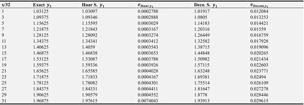
Table 3. Comparison between the error of Haar solution and the error by decomposition method for y1 of Ex. (2) with (J=3).

x/32 Exact ‹_ª Haar S. ‹_ª —«¬¬-,‹ª Deco. S. ‹ª —®—¯°±,‹ª

1 1.03125 1.03097 0.0002788 1.01917 0.012084

3 1.09375 1.09346 0.0002888 1.0805 0.013253

5 1.15625 1.15595 0.0003029 1.14183 0.014421

7 1.21875 1.21843 0.0003167 1.20316 0.01559

9 1.28125 1.28092 0.0003274 1.26449 0.016759

11 1.34375 1.34341 0.0003412 1.32582 0.017928

13 1.40625 1.4059 0.0003543 1.38715 0.019096

15 1.46875 1.46838 0.0003653 1.44848 0.020265

17 1.53125 1.53087 0.0003788 1.50982 0.021434

19 1.59375 1.59336 0.0003926 1.57115 0.022603

21 1.65625 1.65585 0.0004028 1.63248 0.023771

23 1.71875 1.71833 0.0004167 1.69381 0.02494

25 1.78125 1.78082 0.0004301 1.75514 0.026109

27 1.84375 1.84331 0.0004411 1.81647 0.027278

29 1.90625 1.90579 0.0004552 1.8778 0.028446

Figure 1. The comparison between the Haar solution of BVP and Haar solution of its Integral form in Ex. (1) with J=3.

Figure 2. The effect of increasing the collocation points for Eq. (28).

Figure 3. The effect of the increasing the collocation points for Eq. (30).

Figure 4. The comparison between Haar solution and Decomposition solution for y1 for Ex. (2) with J=3.

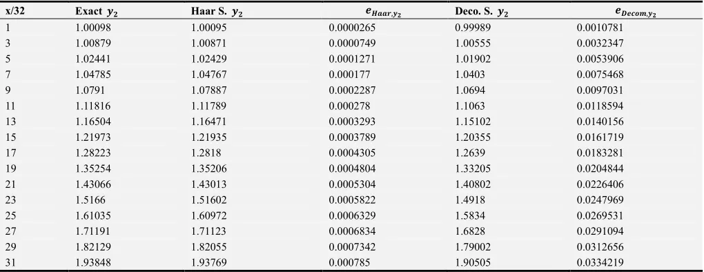
Table 4. Comparison between the error of Haar solution and the error by decomposition method for y2 of Ex. (2) with (J=3).

x/32 Exact ‹² Haar S. ‹² —«¬¬-,‹_² Deco. S. ‹² —®—¯°±,‹_²

1 1.00098 1.00095 0.0000265 0.99989 0.0010781 3 1.00879 1.00871 0.0000749 1.00555 0.0032347 5 1.02441 1.02429 0.0001271 1.01902 0.0053906 7 1.04785 1.04767 0.000177 1.0403 0.0075468 9 1.0791 1.07887 0.0002287 1.0694 0.0097031 11 1.11816 1.11789 0.000278 1.1063 0.0118594 13 1.16504 1.16471 0.0003293 1.15102 0.0140156 15 1.21973 1.21935 0.0003789 1.20355 0.0161719 17 1.28223 1.2818 0.0004305 1.2639 0.0183281 19 1.35254 1.35206 0.0004804 1.33205 0.0204844 21 1.43066 1.43013 0.0005304 1.40802 0.0226406 23 1.5166 1.51602 0.0005822 1.4918 0.0247969 25 1.61035 1.60972 0.0006329 1.5834 0.0269531 27 1.71191 1.71123 0.0006834 1.6828 0.0291094 29 1.82129 1.82055 0.0007342 1.79002 0.0312656 31 1.93848 1.93769 0.000785 1.90505 0.0334219

Table 5. Comparison between Haar solution and differential transform method for Ex. (3).

Method Haar Wavelet Differential Transform [18]

Absolute error 1.9 ∗ 10 l 7.3 ∗ 10 5

exac t

B VP

Integral

0.0 0.2 0.4 0.6 0.8 x

0.2 0.4 0.6 0.8 1.0 1.2

y x

1.0 1.5 2.0 2.5 3.0 3.5 4.0 J

0.291 0.292 0.293 0.294 0.295

Error

1.5 2.0 2.5 3.0 3.5 4.0 J

0.000 0.002 0.004 0.006 0.008

Error

exact y1

Haar y1

Decomposition y₁

0.2 0.4 0.6 0.8 x

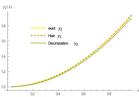
Figure 1. The comparison between Haar solution and Decomposition solution for y2 for Ex. (2) with J=3.

5. Conclusion

Applying the Haar wavelet transform with collocation points method is introduced and we found that:

a) Solving the problem as integral equation is more accurate than solving it as BVP, see table 1 and figure 1.

b) It is observed that if the level of resolution is increased i.e. if the collocation points are increased, then we can get a better solution with less error, see table 2 and figures 2,3.

c) Using Haar wavelet technique to solve the system of integral equations is more efficient than the use of decomposition method, see tables 3, 4 and figures 4, 5. d) The Haar solution of integro-differential equations

gives accuracy more than the differential transform method given in [20], see table 5.

e) It can be concluded that this method is quite suitable, accurate, and efficient in comparison to other classical methods.

References

[1] D. Porter, D. S. G. Stirling, Integral equation a practical treatment, from spectral theory to application, Cambridge University press, 1990.

[2] L. M. Delves, J. L. Mohamed, Computational Methods for Integral Equations, Cambridge University Press, 1985. [3] Youssef, I. K., Ibrahim, R. A. “Boundary value problems,

Fredholm integral equations, SOR and KSOR methods”, Life Science Journal, 10 (2), (2013) 304-312.

[4] H. A. El-Arabawy, I. K. Youssef, A symbolic algorithm for solving linear two-point Boundary value problems by modified Picard technique, Mathematical and Computer Modeling, 49 (2009) 344-351.

[5] E. Babolian, J. Biazar & A. R. Vahidi, The decomposition method applied to systems of Fredholm integral equations of

the second kind, Applied Mathematics and Computation, 148 (2004) 443–452.

[6] K. Maleknejad, N. Aghazadeh & M. Rabbani, Numerical solution of second kind Fredholm integral equations system by using a Taylor-series expansion method, Applied Mathematics and Computation 175 (2006) 1229–1234.

[7] C. F. Chen, C. H. Hsiao, Haar Wavelet Method for solving Lumped and distributed parameter systems, IEEE Proceeding Control Theory Appl., 144 (1) (1997) pp. 87-94.

[8] O. Christensen, K. L. Christensen, Approximation Theory from Taylor Polynomials to Wavelets, Birkhauser Boston, ISBN 0-8176-3600-5, 2004.

[9] U. Lepik, H. Hein, Haar wavelet with applications, Springer international Publishing Switzerland, ISSN 2192-4732, 2014. [10] U. Lepik, E. Tamme, Application of the Haar wavelets for

solution of linear integral equations, Dynamical Systems and Applications, Antalaya, Proceedings (2005) pp. 494–507. [11] U. Lepik, Application of Haar wavelet transform to solving

integral and differential equations, Applied Mathematics and Computation, 57 (1) (2007) pp. 28-46.

[12] S. Islam, I. Aziz & B. Sarler, Numerical Solution of second order boundary value problems by collocation method with Haar Wavelets, Mathematical and Computer Modeling, 52 (2010) pp. 1577-1590.

[13] U. Lepik, Numerical solution of differential equations using Haar wavelets, Mathematics and Computers in Simulation, 68 (2005) pp. 127-143.

[14] I. K. Youssef, A. R. A. Ali. Memory Effects in Diffusion like Equation via Haar Wavelets. Pure and Applied Mathematics Journal 5 (4) 2016 130-140. Doi: 0.11648/j.pamj.20160504.17. [15] I. K. Youssef, M. H. El Dewaik. Haar Wavelet Solution of Poisson’s Equation and Their Block Structures. American Journal of Mathematical and Computer Modelling, 2 (3) (2017) 88-94. Doi: 10.11648/j.ajmcm.20170203.11.

[16] U. Lepik, Numerical Solution of evolution equations by the Haar wavelet method, Applied Mathematics and Computation, 185 (2006) pp. 695-704.

[17] I. K. Youssef, Sh. A. Meligy, Boundary value problems on triangular domains and MKSOR methods, Applied and Computational Mathematics, sciencepublishinggroup, 3 (3) (2014) 90-99.

[18] U. Lepik, Haar wavelet method for nonlinear integro-differential equations, Applied Mathematics and Computation 176 (2006) 324–333.

[19] S. N. HA, C. R. LEE, Numerical study for two-point boundary value problems using Green function, Computer and Mathematics with Applications, 44 (2002) 1599-1608. [20] P. Darania, Ali Ebadian. “ A method for the numerical solution

of the integro-differential equations”, Applied Mathematics and Computation 188 (2007) 657–668.

exact y2

Haar y₂

Decomposition y₂

0.2 0.4 0.6 0.8 x