Photonic Delay Systems as Machine Learning
Implementations
Michiel Hermans [email protected]
OPERA - Photonics Group Universit´e Libre de Bruxelles
Avenue F. Roosevelt 50, 1050 Brussels, Belgium
Miguel C. Soriano [email protected]
Instituto de F´ısica Interdisciplinar y Sistemas Complejos, IFISC (UIB-CSIC) Campus Universitat de les Illes Balears
E-07122 Palma de Mallorca, Spain
Joni Dambre [email protected]
ELIS departement Ghent University
Sint Pietersnieuwstraat 41, 9000 Ghent, Belgium
Peter Bienstman [email protected]
INTEC departement Ghent University
Sint Pietersnieuwstraat 41, 9000 Ghent, Belgium
Ingo Fischer [email protected]
Instituto de F´ısica Interdisciplinar y Sistemas Complejos, IFISC (UIB-CSIC) Campus Universitat de les Illes Balears
E-07122 Palma de Mallorca, Spain
Editor:Yoshua Bengio
Abstract
Nonlinear photonic delay systems present interesting implementation platforms for machine learning models. They can be extremely fast, offer great degrees of parallelism and poten-tially consume far less power than digital processors. So far they have been successfully employed for signal processing using the Reservoir Computing paradigm. In this paper we show that their range of applicability can be greatly extended if we use gradient descent with backpropagation through time on a model of the system to optimize the input encod-ing of such systems. We perform physical experiments that demonstrate that the obtained input encodings work well in reality, and we show that optimized systems perform signifi-cantly better than the common Reservoir Computing approach. The results presented here demonstrate that common gradient descent techniques from machine learning may well be applicable on physical neuro-inspired analog computers.
1. Introduction
Applied research in neural networks is currently strongly influenced by available computer architectures. Most strikingly, the increasing availability of general-purpose graphical pro-cessing unit (GPGPU) programming has sped up the computations required for training (deep) neural networks by an order of magnitude. This development allowed researchers to dramatically scale up their models, in turn leading to the major improvements on state-of-the-art performances on tasks such as computer vision (Krizhevsky et al., 2012; Cire¸san et al., 2010).
One class of neural models which has only seen limited effects of the boost in speed from GPUs are recurrent models. Recurrent neural networks (RNNs) are very interesting for processing time series, as they can take into account an arbitrarily long context of their in-put history. This has important implications in tasks such as natural language processing, where the desired output of the system may depend on context that has been presented to the network a relatively long time ago. In common feedforward networks such dependen-cies are very hard to include without scaling up the model to an impractically large size. Recurrent networks, however, can–at least in principle–carry along relevant context as they are being updated.
In practice, recurrent models suffer from two important drawbacks. First of all, where feedforward networks fully benefit from massively parallel architectures in terms of scal-ability, recurrent networks, with their inherently sequential nature do not fit so well into this framework. Even though GPUs have been used to speed up training RNNs (Sutskever et al., 2011; Hermans and Schrauwen, 2013), the total obtainable acceleration for a given GPU architecture will still be limited by the number of sequential operations required in an RNN, which is typically much higher than in common neural networks. The second issue is that training RNNs is a notoriously slow process due to problems associated with fading gradients, which is especially cumbersome if the network needs to learn long-term dependencies within the input time series. Recent attempts to solve this problem using the Hessian-free approach have proved promising (Martens and Sutskever, 2011). Other attempts using stochastic gradient descent combined with more heuristic ideas have been described in Bengio et al. (2013).
In this paper we will consider a radical alternative to common, digitally implemented RNNs. A steadily growing branch of research is concerned withReservoir Computing (RC), a con-cept which employs high-dimensional, randomly initialized dynamical systems (termed the
electro-optical devices (Larger et al., 2012; Paquot et al., 2012), fully electro-optical devices (Brunner et al., 2013) and nanophotonic circuits (Vandoorne et al., 2008, 2014). As opposed to digital im-plementations, physical systems can offer great speed-ups, inherent massive parallelism, and great reductions in power consumption. In this sense, physical dynamical systems as ma-chine learning implementation platforms may one day break important barriers in terms of scalability. In the near future, especially optical computing devices might find applications in several tasks where fast processing is essential, such as in optical header recognition, optical signal recovery, or fast control loops.
The RC paradigm, despite its notable successes, still suffers from an important drawback. Its inherently unoptimized nature makes it relatively inefficient for many important machine learning problems. When the dimensionality of the input time series is low, the expansion into a high-dimensional nonlinear space offered by the reservoir will provide a sufficiently di-verse set of features to approximate the desired output. If the input dimensionality becomes larger, however, relying on random features becomes increasingly difficult as the space of possible features becomes so massive. Here, optimization with gradient descent still has an important edge over the RC concept: it can shape the necessary nonlinear features auto-matically from the data.
In this paper we aim to integrate the concept of gradient descent in neural networks with physically implemented analog machine learning models. Specifically, we will employ a physical dynamical system that has been studied extensively from the RC paradigm, a delayed feedback electro-optical system (Larger et al., 2012; Paquot et al., 2012; Soriano et al., 2013). In order to use such a system as a reservoir, an input time series is encoded into a continuous time signal and subsequently used to drive the dynamics of the physical setup. The response of the device is recorded and converted to a high-dimensional feature set, which in turn is used with linear regression in the common RC setup. In this particular case, the randomness of RC is incorporated in the input encoding. This encoding is per-formed offline on a computer, but is usually completely random. Even though efforts have been performed to improve this encoding in a generic way (by ensuring a high diversity in the network’s response, discussed in Rodan and Tino (2011) and Appeltant et al. (2014)), a way to create task-specific input encodings is still lacking.
In Hermans et al. (2014b), the possibility to use backpropagation through time (BPTT) (Rumelhart et al., 1986) as a generic optimization tool for physical dynamical systems was addressed. It was found that BPTT can be used to find remarkably intricate solutions to complicated problems in dynamical system design. In Hermans et al. (2014a) simulated results of BPTT used as an optimization method for input encoding in the physical sys-tem described above were presented. In this paper we go beyond this work and show for the first time experimental evidence that model-based BPTT is a viable training strategy for physical dynamical systems. We choose two often-used high-dimensional data sets for validation, and we show that input encoding that is optimized using BPTT in a common machine learning approach, provides a significant boost in performance for these tasks when compared to random input encodings. This not only demonstrates that machine learning approaches are more broadly applicable than is generally assumed, but also that physical analog computers can in fact be considered as parametrizable machine learning models, and may play a significant role in the next generation of signal processing hardware.
corre-sponding model in detail. We explain how we convert the continuous-time dynamics of the system into a discrete-time update equation which we use as model in our simulation. Next, we present and analyze the results on the tasks we considered and compare experimental and simulated results.
2. Physical System
In this section we will explain the details of the physical system. We will start by formally introducing its delay dynamics operating in continuous time. Next, we will explain how the feedback delay can be used for realizing a high-dimensional state space encoded in time, and we demonstrate that–combined with special input and output encoding–the setup can be seen as a special case of RNN. Finally we explain how we discretize the system’s input and output encoding, which enables us to approximate the dynamics of the system by a discrete-time update equation.
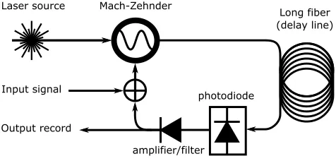
The physical system we employ in this paper is a delayed feedback system exhibiting Ikeda-type dynamics (Larger et al., 2004; Weicker et al., 2012). We provide a schematic depiction of the physical setup in Figure 1. It consists of a laser source, a Mach-Zehnder modulator, a long optical fiber (≈4 km) which acts as a physical delay line, and an electronic circuit which transforms the optical beam intensity in the fiber into a voltage. This voltage is amplified and low-pass filtered and can be measured to serve as the system output. Moreover, it is added to an external input voltage signal, and then serves as the driving signal for the Mach-Zehnder modulator. The measured output signal is well described by the following differential equation (Larger et al., 2012):
Ta˙(t) =−a(t) +βsin2(a(t−D) +z(t) +φ)−1/2. (1)
Here, the signala(t) corresponds to a measured voltage signal (down to a constant scaling and bias factor). The factor T is the time scale of the low-pass filtering operation in the electronic circuit, equal to 0.241 µs, β is the total amplification in the loop, which in the experiments can be varied by changing the power of the laser source. D is the delay of the system, which has been chosen as 20.82 µs. z(t) is the external input signal, and φ is a constant offset phase (which can be controlled by setting a bias voltage), which we set at π/4 for all results presented in this paper. For ease of notation we will call the system a
delay-coupled Mach-Zehnder, which we abbreviate as DCMZ.
2.1 Input and Output Encoding
Delay-coupled systems have–in principle–an infinite-dimensional state space, as these sys-tems directly depend on their full history covering an interval of one delay time. This prop-erty has been the initial motivation for using delay-coupled systems in the RC paradigm in the past years. Suppose we have a multivariate input time series, which we will denote by si, for i∈ {1,2,· · ·, S}, S being the total number of instances (the length of the input
sequence). Eachsi is a column vector of size Nin×1, withNinthe number of input
dimen-sions. We wish to construct an accompanying output time seriesyi. We convert each data
point si to a continuous-time segmentzi(t) as follows:
zi(t) =m0(t) +mT(t)si,
where m0(t) and m(t) are masking signals, which are defined fort ∈[0· · ·P], with P the
masking period. The signal m0(t) is scalar, and constitutes a bias signal, and m(t) is a
column vector of size Nin ×1. The total input signal z(t) is then constructed by time-concatenation of the segmentszi(t):
z(t) =zi(tmod P) for t∈ {(i−1)P· · ·iP}.
Similarly, we define an output mask u(t). We divide the state variable time traces a(t) in segments ai(t) of duration P such that
a(t) =ai(t mod P) for t∈ {(i−1)P· · ·iP}.
The output time seriesyi is then defined as
yi=y0+
Z P
0
dt ai(t)u(t). (2)
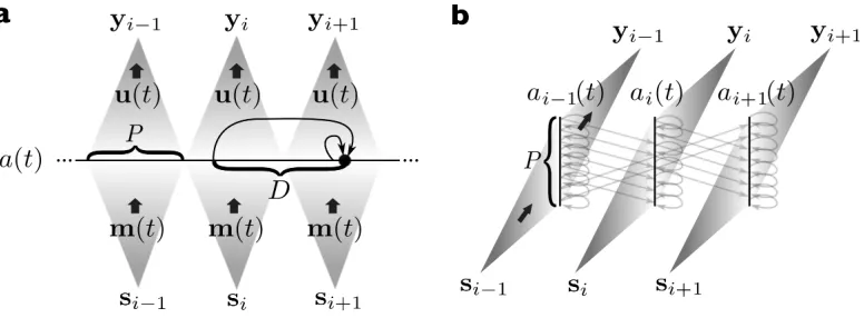
It is possible to see the delay-coupled dynamical system combined with the masking prin-ciple as a special case of an infinite-dimensional discrete-time recurrent neural network, as illustrated in Figure 2. The recurrent weights, connecting the hidden states over time, are fixed, and manifested by the delayed feedback connection. The input and output weights correspond to the input and output masks.
Input signal
Output record
Mach-Zehnder
Laser source Long fiber
(delay line)
photodiode
amplifier/filter
Figure 1: Schematic depiction of a delay-coupled Mach-Zehnder interferometer.
In practice, we cannot measure the state trajectory with infinite time resolution, nor can we produce signals with an arbitrary time dependency, as there will always be constraints that limit the maximum bandwidth of the generated signals. Therefore, we assume that m0(t),m(t) andu(t) all consist of piecewise constant signals1, which are segmented inNm
parts, Nm being the number of masking steps:
m0(t) =m0k for t∈ {(k−1)Pm· · ·kPm},
m(t) =mk for t∈ {(k−1)Pm· · ·kPm},
u(t) =uk for t∈ {(k−1)Pm· · ·kPm}, (3)
where the length of each step is given byPm=P/Nm. This means that we now have a finite
number of parameters that fully determine m0(t), m(t) and u(t). Note that, due to our
choice of P =D,Pm will by definition be an integer number of times the delay lengthD.
This is convenient for the next section, where we will make a discrete-time approximation of the system, but it is not a necessary requirement of the system to perform well.
2.2 Converting the System to a Trainable Machine Learning Model
In Hermans et al. (2014b) it was shown that BPTT can be applied to models of continuous-time dynamical systems. Indeed, it is perfectly possible to simulate the system using differ-ential equation solvers and consequently compute parameter gradients. One issue, however, is the significant computational cost. Note that, in a common discrete-time RNN, a single state update corresponds to a single matrix-vector multiplication and the application of a nonlinearity. In our case it involves the sequential computation of the full time trace of ai(t). This is considerably more costly to compute, especially given the fact that–as in most
gradient descent algorithms–we may need to compute it on large amounts of data and this for multiple thousands of iterations.
Due to the piecewise constant definition ofu(t) we can make a good approximation ofa(t).
Figure 2: Schematic representation of the masking principle. a: Depiction of the input time series si and the way it is converted into a continuous-time signal by means of
the input masking signalsm(t). The horizontal line in the middle shows the time evolution of the system state a(t). We have depicted two connection arrows at one point in time, which indicate thata(t) depends on its immediately preceding value (due to the low-pass filtering operation), and its delayed value. The state trajectories are divided into segments each of which are projected to an output instance yi. b: The same picture as in panel a, but now represented as a
time-unfolded RNN. We have shown the connections between the states as light grey arrows, but note that there are in principle infinitely many connections.)
First we combine Equations 2 and 3. This gives us:
yi= Nm
X
k=1
Z kPm
(k−1)Pm
dtukai(t) = Nm
X
k=1 uk¯aik,
where ¯aik =
RkPm
(k−1)Pmdt ai(t). This means that we can represent ai(t) by a finite set of variables ¯aik. To represent the full time trace of a(t) we adopt a simplified notation as
follows2: ¯aj = ¯aik, wherej= (i−1)Nm+k.
Now we make the following approximation: we assume that for the duration of a single masking step, we can replace the term a(t−D) by ¯ai−Nm, that is, we consider it to be constant. With this assumption, we can solve Equation 1 for the duration of one masking step:
a(t) =γi+ (ˆai−γi) exp
−t
T
for t∈ {0· · ·Pm}, (4)
with
γi =β
sin2(¯ai−Nm+z(t) +φ)−1/2
,
and ˆai the value of a(t) at the start of the interval. Integrating over the interval t = {0· · ·Pm} we find:
¯
ai= (ˆai−γi)κ+Pmγi,
2. Please do not confuse with the indexiinai(t). Here the index indicates single masking steps, rather
withκ= 1−e−Pm/T. We can eliminate ˆa
i as follows. First we derive from Equation 4 that
ˆ
ai+1= (ˆai−γi)e−Pm/T+γi. If we combine this expression with the following two:
¯
ai= (ˆai−γi)κ+Pmγi,
¯
ai+1= (ˆai+1−γi+1)κ+Pmγi+1,
we can eliminate ˆai, and we end up with the following update equation for ¯ai:
¯
ai+1 =ρo¯ai+ρ1γi+ρ2γi+1,
withρ0 = e−Pm/T,ρ1=T κ−Pme−Pm/T, andρ2=Pm−T κ. This leads to a relatively
quick-to-compute update equation to simulate the system. BPTT can also be readily applied on this formula, as it is a simple update equation just like for a common RNN. This is the simulation model we used for training the input and output masks of the system.
We verified the accuracy of this approximation both on measured data of the DCMZ and on a highly accurate simulation of the system. For the parameters used in the DCMZ we got very good correspondence with the model (obtaining a correlation coefficient between simulated and measured signals of 99.6%).
2.3 Hybrid Training Approach
One challenge we faced when trying to match the model with the experimentally measured data was that we obtained a sufficiently good correspondence only when we very carefully fitted the values for β and φ. We can physically control these parameters, but exactly setting their numerical values turned out not to be trivial in the experiments, especially since they tend to show slight drifting behavior over longer periods of time (in the order of hours). As a consequence, it turned out to be a challenge to train parameters in simulation, and simply apply them directly on the DCMZ. Therefore, we applied a hybrid approach between gradient descent and the RC approach. We train both the input and output masks in simulations. Next, we only use the input masks for the physical setup. After recording all the data, we retrained the output weights using gradient descent, this time on the measured data itself. The idea is that the input encoding will produce highly useful features for the system even when it is trained on a model that may show small, systematic differences with the physical setup.
2.4 Input Limitations
addition of the input signal with the delayed feedbacka(t−D), there is still a chance that the total argument falls out of the range [−π/2· · ·π/2], but in practice such occurrences turned out to be rare, and could safely be ignored.
3. Experiments
We tested the use of BPTT for training the input masks both in simulation and in exper-iment on two benchmark tasks. First, we considered the often-used MNIST written digit recognition data set, where we use the dynamics of the system indirectly. Next, we applied it on the TIMIT phoneme data set. For the MNIST experiment we usedNm = 400 masking
steps. For TIMIT we usedNm = 600.
3.1 MNIST
To classify static images using a dynamical system, we follow an approach similar to the one introduced in Rolfe and LeCun (2013). Essentially, we repeat the same input segment several times until the state vector ai(t) of the DCMZ no longer changes. Next we choose
the final instance of ai(t) to classify the image. In practice we used 10 iterations for each
image in the MNIST data set (i.e., each input digit is repeated for 10 masking periods). This sufficed for ai(t) to no longer depend on its initial conditions, and in practice this
meant that we were able to present all digits to the network right after each other.
Input masks were trained using 106training iterations, where for each iteration the gradient was determined on 500 randomly sampled digits. For training we used Nesterov momen-tum (Sutskever et al., 2013), with momenmomen-tum coefficient 0.9, and a learning rate of 0.01 which linearly decayed to zero over the duration of the training. As regularization we only performed 1-pixel shifts for the digits. Note that these 1-pixel shifts were used for training the input masks, but we did not include them when retraining the output weights, as we only presented the DCMZ with the original 60,000 training examples.
After training the input weights, we gathered both physical and simulated data for the 4 experiments as described below, and retrained the output weights to obtain a final score. Output weights are trained using the cross-entropy loss function over 106 training iterations, where for each iteration the gradient was determined on 1000 randomly sampled digits. We again used Nesterov momentum, with momentum coefficient 0.9. The learning rate was chosen at 0.002 and linearly decayed to zero. Meta-parameter optimization was performed using 10,000 randomly selected examples from the training set.
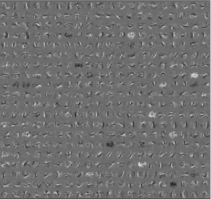
We performed 4 tests on MNIST. First of all we directly compared performances between the simulated and experimental data. When we visualized the features that the trained input masks generated, we noticed that they seemed ordered (see Figure 3). Indeed, for each masking step, a single set of weightsmk, which can be seen as a receptive field, is
ap-plied to the input image, and the resulting signals from the receptive fields are injected into the physical setup one after each other. Apparently, the trained input masks have similar features grouped together in time. To confirm that this ordering in time is a purposeful property, we shuffled the features mk over a single masking period to obtain a new input
Masking steps
input channels
100 200 300 400 500 600
5
10
15
20
25
30
35
40
Figure 4: Depiction of the input mask trained on the TIMIT task. We have shown the input weights of the 600 masking steps (horizontal axis) for each channel (vertical axis). For the sake of visualization we have here depicted the natural logarithm of the absolute value of the mask plus 0.1. This enhances the difference in scaling for the different channels.
MNIST test error TIMIT frame error rate
Experimental data 1.16% 33.2%
Simulated data 1.08% 31.7%
Simulated data: time-shuffled 1.41% 32.8%
Simulated data: random 6.72% 40.5%
Best in literature 0.23% 25.0%
(Cire¸san et al., 2012) (Cheng et al., 2009)
Table 1: Benchmark performances for different experimental setups.
was optimized (which is the RC approach).
Results are presented in the middle column of Table 1. The difference between experimental and simulation results is very small. The time shuffled features do indeed cause a notable increase in the classification error rate, indicating that the optimized input masks actively make use of the internal dynamics of the system, and not just offer a generically good fea-ture set.
3.2 TIMIT
We applied frame-wise phoneme recognition to the TIMIT data set (Garofolo et al., 1993). The data was pre-processed to 39-dimensional feature vectors using Mel Frequency Cepstral Coefficients (MFCCs). The data consists of the log energy, and the first 12 MFCC coeffi-cients, enhanced with their first and second derivative (the so-called delta and delta-delta features). The phonemes were clustered into a set of 39 classes, as is the common approach. Note that we did not include the full processing pipeline to include segmentation of the labels and arrive at a phoneme error rate. Here, we wish to illustrate the potential of our approach and demonstrate how realizations of physical computers can be extended to fur-ther concepts, rafur-ther than to claim state-of-the-art performance. Given that, in addition, the input masks are trained to perform frame-wise phoneme classification, including the whole processing pipeline would not be informative.
Input masks are trained using 50,000 training iterations, where for each iteration the gra-dient was determined on 200 randomly sampled sequences of a length of 50 frames. For training we again used Nesterov momentum, with momentum coefficient 0.9, and a learning rate of 0.2 which linearly decayed to zero over the duration of the training. As we were in a regime far from overfitting, we simply chose the training error for meta-parameter opti-mization. We have depicted the optimized input mask in Figure 4. Note that the training process strongly rescaled the masking weights for different input channels, putting more emphasis on the delta and delta-delta features (respectively channels 14 to 26 and 27 to 39 ).
We repeated the four scenarios previously discussed: using optimized masks in simulation and experiment, using time-shuffled masks, and using random masks. The resulting frame error rates are presented in the right column of Table 1. The simulated and experimental data differ by 1.5%, a relatively small difference, indicating that input masks optimized in simulation are useful in practice, even in the presence of unavoidable discrepancies between the used model and the DCMZ. Results for random masks are significantly worse than those with optimized input masks.
Comparison to literature is not straightforward as most publications do not mention frame error rate, but rather the error rate after segmentation. We included the lowest frame error rate mentioned in literature to our knowledge, though it should be stated that other works may have even lower values, even when they are not explicitly mentioned. For an overview of other results on frame error rate please check Keshet et al. (2011).
The decrease in performance when using time-shuffled masks is quite modest, suggesting that in this case, most of the improvement over random masks is due directly from the features themselves, and the precise details of the dynamics of the system are less crucial than was the case in the MNIST task3. Although further testing is needed, we suggest two possible reasons for this. First of all, the TIMIT data set we used contained the first and second derivatives of the first thirteen channels, which already provides information on the preceding and future values and acts as an effective time window. Indeed as can be seen from Figure 4, the input features amplify these derivatives. Therefore, a lot of temporal
context is already embedded in a single input frame, reducing the need for recurrent con-nections. Secondly, the lack of control over the way information is mixed over time may still pose an important obstacle to effectively use the recurrence in the system. Currently, input features are trained to perform two tasks at once: provide a good representation of the current input, and at the same time design the features in such a way that they can make use of the (fixed) dynamics present within the system. It may prove the case that the input masks do not have enough modeling power to fulfill both tasks at once, or that the way temporal mixing occurs in the network cannot be effectively put to use for this particular task.
4. Discussion and Future Work
In this paper we presented an experimental survey of the use of backpropagation through time on a physical delay-coupled electro-optical dynamical system, in order to use it as a machine learning model. We have shown that such a physical setup can be approached as a special case of recurrent neural network, and consequently can be trained with gradient descent using backpropagation. Specifically, we have shown that both the input and output encodings (input and output masks) for such a system can be fully optimized in this way, and that the encodings can be successfully applied to the real physical setup.
Previous research in the usage of electro-optical dynamical systems for signal processing used random input encodings, which are quite inefficient in scenarios where the input di-mensionality is high. We focused on two tasks with a relatively high input didi-mensionality: the MNIST written digit recognition data set and the TIMIT phoneme recognition data set. We showed that in both cases, optimizing the input encoding provides a significant performance boost over random masks. We also showed that the input encoding for the MNIST data set seems to directly utilize the inherent dynamics of the system, and hence does more than simply provide a useful feature set.
Note that the comparison with Reservoir Computing is based on the constraints by a given physical setup and a given set of resources. We note that the Reservoir Computing setup could give good results on the proposed tasks too, if we were greatly scaling up its effec-tive dimensionality. This has been evidenced in, for example, Triefenbach et al. (2010), where good results on the TIMIT data set were achieved by using Echo State Networks (a particular kind of Reservoir Computing) of up to 20,000 nodes. In our setup this would be achieved by increasing the number of masking steps Nm within one masking period.
In reality, however, we will face two practical problems. First of all, there are bandwidth limitations in signal generation and measurement. Parts of the signal that fluctuate rapidly would be lost when reducing the duration of a single masking step. If one would scale up by keeping the length of the mask steps fixed but use a longer physical delay, for instance a fiber of tens or hundreds of kilometers, the potential gain in performance comes at the cost of one of the systems important advantages: its speed. Also it is hard to foresee how other optical effects in such long fibers such as dispersion and attenuation, would affect performance. This would be an interesting research topic for future investigations.
when the model becomes less acute.
Several directions for future improvements are apparent. The most obvious one is that we could greatly simplify the training process by putting the DCMZ measurements directly in the training loop: instead of optimizing input masks in simulations, we could just as well directly use real, measured data. The Jacobians required for the backpropagation phase can be computed from the measured data. A training iteration would then consist of the following steps: sample data, produce the corresponding input to the DCMZ with the cur-rent input mask, measure the output, perform backpropagation in simulation, and update the parameters. The benefit would be that we directly end up with functional input and output masks, without the need for retraining. On top of that, data collection would be much faster. The only additional requirement for this setup would be the need for a single computer controlling both signal generation and signal measurement.
The next direction for improvement would be to rethink the design of the system from a machine learning perspective. The current physical setup on which we applied backprop-agation finds its origins in reservoir computing research. As we argue in Section 2, the system can be considered as a special case of recurrent network with a fixed, specific con-nection matrix between the hidden states at different time steps. In the reservoir computing paradigm, one always uses fixed dynamical systems that remain largely unoptimized, such that in the past this fact was not particularly restrictive. However, given the possibility of fully optimizing the system that was demonstrated in this paper, the question on how to redesign this system such that we can assert more control over the recurrent connection matrix, and hence the dynamics of the system itself, becomes far more relevant. Currently we have a fixed dynamical system of which we optimize the input signal to accommodate a certain signal processing task. As explained at the end of Section 3.2, it appears that backpropagation can currently only leverage the recurrence of the system to a limited de-gree, when using a single delay loop. Therefore it would be more desirable to optimize both the input signal and the internal dynamics of the system to accommodate a certain task. Alternatively, the configuration can be easily extended to multiple delay loops, allowing for a richer recurrent connectivity.
The most significant result of this paper is that we have shown experimentally that the backpropagation algorithm, a highly abstract machine learning algorithm, can be used as a tool in designing analog hardware to perform signal processing. This means that we may be able to vastly broaden the scope of research into physical and analog realizations of neural architectures. In the end this may result in systems that combine the best of both worlds: powerful processing capabilities at a tremendous speed and with a very low power consumption.
Acknowledgements
from the Universitat de les Illes Balears for an Invited Young Researcher Grant. In addition, we acknowledge Prof. L. Larger for developing the optoelectronic delay setup.
References
Lennert Appeltant, Guy Van der Sande, Jan Danckaert, and Ingo Fischer. Constructing optimized binary masks for reservoir computing with delay systems. Scientific Reports, 4:3629, 2014.
Yoshua Bengio, Nicolas Boulanger-Lewandowski, and Razvan Pascanu. Advances in opti-mizing recurrent networks. In Acoustics, Speech and Signal Processing (ICASSP), 2013 IEEE International Conference on, pages 8624–8628. IEEE, 2013.
Daniel Brunner, Miguel C Soriano, Claudio R Mirasso, and Ingo Fischer. Parallel photonic information processing at gigabyte per second data rates using transient states. Nature Communications, 4:1364, 2013.
Ken Caluwaerts, Michiel D’Haene, David Verstraeten, and Benjamin Schrauwen. Loco-motion without a brain: physical reservoir computing in tensegrity structures. Neural Computation, 19(1):35–66, 2013.
Chih-Chieh Cheng, Fei Sha, and Lawrence Saul. A fast online algorithm for large margin training of online continuous density hidden markov models. In Interspeech 2009, pages 668–671, 2009.
Dan Cire¸san, Ueli Meier, Luca Maria Gambardella, and J¨urgen Schmidhuber. Deep, big, simple neural nets for handwritten digit recognition. Neural Computation, 22(12):3207– 3220, 2010.
Dan Cire¸san, Ueli Meier, and J¨urgen Schmidhuber. Multi-column deep neural networks for image classification. In Computer Vision and Pattern Recognition (CVPR), 2012 IEEE Conference on, pages 3642–3649. IEEE, 2012.
Chrisantha Fernando and Sampsa Sojakka. Pattern recognition in a bucket. InProceedings of the 7th European Conference on Artificial Life, pages 588–597, 2003.
John Garofolo, National Institute of Standards, Technology (US, Linguistic Data Con-sortium, Information Science, Technology Office, United States, and Defense Advanced Research Projects Agency). TIMIT Acoustic-phonetic Continuous Speech Corpus. Lin-guistic Data Consortium, 1993.
Helmut Hauser, Auke J Ijspeert, Rudolf M F¨uchslin, Rolf Pfeifer, and Wolfgang Maass. Towards a theoretical foundation for morphological computation with compliant bodies.
Optics Express, 105(5-6):355–370, 2011.
Michiel Hermans, Joni Dambre, and Peter Bienstman. Optoelectronic systems trained with backpropagation through time. IEEE Transactions in Neural Networks and Learning Systems, 2014a. in press.
Michiel Hermans, Benjamin Schrauwen, Peter Bienstman, and Joni Dambre. Automated design of complex dynamic systems. PloS One, 9(1):e86696, 2014b.
Herbert Jaeger. Short term memory in echo state networks. Technical Report GMD Report 152, German National Research Center for Information Technology, 2001.
Herbert Jaeger and Harald Haas. Harnessing nonlinearity: predicting chaotic systems and saving energy in wireless telecommunication. Science, 308:78–80, April 2 2004.
Joseph Keshet, David McAllester, and Tamir Hazan. Pac-bayesian approach for minimiza-tion of phoneme error rate. In IEEE International Conference on Acoustics, Speech and Signal Processing, pages 2224–2227, 2011.
Alex Krizhevsky, Ilya Sutskever, and Geoff Hinton. Imagenet classification with deep con-volutional neural networks. In Advances in Neural Information Processing Systems 25, pages 1106–1114, 2012.
Laurent Larger, Jean-Pierre Goedgebuer, and Vladimir Udaltsov. Ikeda-based nonlinear delayed dynamics for application to secure optical transmission systems using chaos.
Comptes Rendus Physique, 5(6):669–681, 2004.
Laurent Larger, Miguel C Soriano, Daniel Brunner, Lennert Appeltant, Jose M Guti´errez, Luis Pesquera, Claudio R Mirasso, and Ingo Fischer. Photonic information processing beyond turing: an optoelectronic implementation of reservoir computing. Optics Express, 3:20, 2012.
Mantas Lukosevicius and Herbert Jaeger. Reservoir computing approaches to recurrent neural network training. Computer Science Review, 3(3):127–149, 2009.
Wolfgang Maass, Thomas Natschl¨ager, and Henri Markram. Real-time computing without stable states: A new framework for neural computation based on perturbations. Neural Computation, 14(11):2531–2560, 2002.
James Martens and Ilya Sutskever. Learning recurrent neural networks with hessian-free optimization. In Proceedings of the 28th International Conference on Machine Learning (ICML-11), pages 1033–1040, 2011.
Yvan Paquot, Francois Duport, Antoneo Smerieri, Joni Dambre, Benjamin Schrauwen, Marc Haelterman, and Serge Massar. Optoelectronic reservoir computing. Scientific Reports, 2:1–6, 2012.
Ali Rodan and Peter Tino. Minimum complexity echo state network. Neural Networks, IEEE Transactions on, 22(1):131–144, 2011.
Jason Tyler Rolfe and Yann LeCun. Discriminative recurrent sparse auto-encoders. In
David Rumelhart, Geoffrey Hinton, and Ronald Williams.Learning internal representations by error propagation. MIT Press, Cambridge, MA, 1986.
Miguel C Soriano, Silvia Ort´ın, Daniel Brunner, Laurent Larger, Claudio Mirasso, Ingo Fischer, and Lu´ıs Pesquera. Opto-electronic reservoir computing: tackling noise-induced performance degradation. Optics Express, 21(1):12–20, 2013.
Jochen Steil. Backpropagation-Decorrelation: Online recurrent learning with O(N) com-plexity. In Proceedings of the International Joint Conference on Neural Networks, vol-ume 1, pages 843–848, 2004.
Ilya Sutskever, James Martens, and Geoffrey Hinton. Generating text with recurrent neural networks. In Proceedings of the 28th International Conference on Machine Learning, pages 1017–1024, 2011.
Ilya Sutskever, James Martens, George Dahl, and Geoffrey Hinton. On the importance of initialization and momentum in deep learning. In Proceedings of the 30th International Conference on Machine Learning (ICML-13), pages 1139–1147, 2013.
Fabian Triefenbach, Azaraksh Jalalvand, Benjamin Schrauwen, and Jean-Pierre Martens. Phoneme recognition with large hierarchical reservoirs. In Advances in Neural Informa-tion Processing Systems 23, pages 2307–2315, 2010.
Kristof Vandoorne, Wouter Dierckx, Benjamin Schrauwen, David Verstraeten, Roel Baets, Peter Bienstman, and Jan van Campenhout. Toward optical signal processing using photonic reservoir computing. Optics Express, 16(15):11182–11192, 2008.
Kristof Vandoorne, Pauline Mechet, Thomas Van Vaerenbergh, Martin Fiers, Geert Mor-thier, David Verstraeten, Benjamin Schrauwen, Joni Dambre, and Peter Bienstman. Ex-perimental demonstration of reservoir computing on a silicon photonics chip. Artificial Life, 5, 2014.