Nonparametric Network Models for Link Prediction
Sinead A. Williamson [email protected] Department of Statistics and Data Science/
Department of Information, Risk and Operations Management, University of Austin at Texas
Editor:Edo Airoldi
Abstract
Many data sets can be represented as a sequence of interactions between entities—for example communications between individuals in a social network, protein-protein interac-tions or DNA-protein interacinterac-tions in a biological context, or vehicles’ journeys between cities. In these contexts, there is often interest in making predictions about future interac-tions, such as who will message whom.
A popular approach to network modeling in a Bayesian context is to assume that the observed interactions can be explained in terms of some latent structure. For example, traffic patterns might be explained by the size and importance of cities, and social network interactions might be explained by the social groups and interests of individuals. Unfor-tunately, while elucidating this structure can be useful, it often does not directly translate into an effective predictive tool. Further, many existing approaches are not appropriate for sparse networks, a class that includes many interesting real-world situations.
In this paper, we develop models for sparse networks that combine structure elucidation with predictive performance. We use a Bayesian nonparametric approach, which allows us to predict interactions with entities outside our training set, and allows the both the latent dimensionality of the model and the number of nodes in the network to grow in expectation as we see more data. We demonstrate that we can capture latent structure while maintaining predictive power, and discuss possible extensions.
Keywords: Dirichlet process, networks, Bayesian nonparametrics, Gibbs sampling, hier-archical modeling
1. Introduction
We are often interested in characterizing and predicting the interactions between objects, be they individuals within an organization, proteins within a cell, or transportation hubs within a region. We can represent these objects as nodes in a network, with the non-zero edges of the network describing the interactions between nodes. For example, we can represent a social network as a binary network, where each node corresponds to an individual, and an edge between nodes corresponds to a friendship between individuals. Patterns of email communication can be modeled using an integer-valued network, with integer-valued edges representing the number of emails sent from one individual to another. Interactions between proteins can be represented using a real-valued network, where the nodes correspond to proteins and the edges correspond to interaction strength.
and Wong, 1987; Snijders and Nowicki, 1997), where each node is assumed to belong to one ofK latent groups, and the interaction between two nodes depends only on their group assignments. This basic model can be extended by allowing the number of latent groups to be unbounded, as in the infinite relational model (IRM, Kemp et al., 2006), or by allowing each node to exhibit membership in multiple latent groups, as in the mixed membership stochastic blockmodel (MMSB, Airoldi et al., 2008). One thing that these models have in common is that they treat nodes as exchangeable, and assume that there exists a fixed, stationary network between these nodes. Each node is represented by the totality of its interactions with other nodes, and we use this information to cluster (or, in the case of the MMSB, co-cluster) the data into distinct groups.
In this paper we follow a different approach: we treat the interactions, rather than the nodes, as data points, and construct an exchangeable sequence of directed binary links. Each link corresponds to a single interaction—such as “friending” or “liking” in a social network, or sending a single email—and is characterized in terms of an ordered pair of nodes. We may observe multiple links between two nodes; this corresponds to repeated interactions (for example, sending multiple emails).
This approach has a number of advantages. Unlike the stochastic blockmodel family, the approach described in this paper allows us to model sparse graphs, where the number of non-zero entries grows asO(M), whereM is the number of nodes. Sparsity is a property of many real-life networks, which tend to exhibit small-world behavior (Caron and Fox, 2015; Orbanz and Roy, 2014).
Another advantage is that our model is explicitly designed for the prediction task. In many scenarios, we might be interested in what the next interaction will be: who will email whom, for example. Stochastic blockmodels aim to model a fully observed network, where the absence of an observed edge is interpreted as an explicitly observed zero. In this set-ting, any predictions must directly contradict these observed zeros. While it is possible to explicitly mark edges as “missing”, we can only do this for a small subset of unobserved edges—if we assume all zero edges in a stochastic blockmodel are in fact unobserved, the maximum likelihood network will have all the edges equal to one. Conversely, by construct-ing an integer-valued network via an exchangeable sequence of links, we frame our problem in a manner that directly provides a predictive distribution over the location of the next link, and allows us to continuously update our posterior predictive distribution in the face of new data. Further, by choosing to place a nonparametric distribution over the sequence of links, we can easily incorporate previously unseen nodes, without any prior knowledge of the number of such nodes.
A further advantage is seen in the computational complexity of the model. Under a stochastic blockmodel with M nodes and K clusters, the computational cost of evaluating the likelihood of the ith node belonging to the kth cluster grows as O(M), meaning that the overall computational cost of inferring the cluster allocations, without resorting to approximations, scales as O(M2K). Conversely, under the proposed model, the cluster likelihood for a link involves only the two nodes associated with the interaction, yielding
This paper begins by examining existing Bayesian network models in Section 2, before going on to present our model in Section 3. We begin by introducing the Dirichlet network distribution in Section 3.1, before proceeding to describe how a mixture of such distribu-tions can create a flexible network model with interesting latent structure in Section 3.2. While the focus of this paper is on integer-valued networks, we also consider extensions to the binary case in Section 3.3. While the primary method we consider does not ex-hibit exchangeable links, we can sample an auxiliary integer-value network and leverage its exchangeability to obtain predictive distributions. In Section 4, we describe an MCMC sampler for the mixture of Dirichlet network distributions, before presenting experimental results in Section 5.
1.1 Notation
We will use the notationZ to represent anM×M network, with elementszsr ∈Nindicating
the relationship between nodess andr. Ifzsr∈ {0,1}, then a non-zero value indicates the
presence of a relationship. Ifzsris allowed to take on arbitrary non-negative integer values, we take this to indicate the number of interactions (for example, emails in a social network, packages in a computer network) between nodes s and r. Unless otherwise specified, we will assumeZ to be a directed network, where Z 6=ZT.
It will sometimes be more convenient to represent the matrix Z as a sequence of inter-actions Y =y1, y2, . . ., where each interaction yi consists of an ordered pair of nodes. We can reconstruct the matrix Z by setting zsr = PiI(yi = (s, r)), where I(·) represents an
indicator function, that returns one iff the statement it refers to is true.
2. Related Work
A number of models have been proposed for modeling interactions within a network. In a Bayesian context, most of these models fall under the general category of stochastic blockmodels (SBs), a class of clustering-based models that generate dense networks. We discuss stochastic blockmodels in Section 2.1.
Recently, there has been growing interest in models for sparse networks, where the number of edges grows linearly (rather than quadratically) with the number of nodes. We discuss relevant work in this area in Section 2.2.
2.1 Stochastic Blockmodels and Related Models
The basic stochastic blockmodel (Holland et al., 1983; Wang and Wong, 1987) posits that each node belongs to one of K latent clusters. For each pair (i, j) of clusters there is a cluster-specific distribution over interactions governed by some parameterθi,j; conditioned
0 10 20 30 40 0
10
20
30
40
(a) Latent structure of the stochastic block-model.
0 10 20 30 40 0
10
20
30
40
(b) Sample from the stochastic blockmodel.
Figure 1: A stochastic blockmodel with 5 clusters.
To position SBs in a Bayesian context (Snijders and Nowicki, 1997), we can place ap-propriate conjugate priors on the cluster parameters θi,j and the cluster proportions. For example, a Bayesian version of the standard Bernoulli stochastic blockmodel takes the form
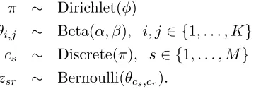
π ∼ Dirichlet(φ)
θi,j ∼ Beta(α, β), i, j∈ {1, . . . , K}
cs ∼ Discrete(π), s∈ {1, . . . , M}
zsr ∼ Bernoulli(θcs,cr).
Figure 1a shows the underlying partitioning of the nodes, with the color of each partition indicating the corresponding value ofθcs,cr in a binary SB. Figure 1b shows an instantiation of a network generated from this structure.
The basic stochastic blockmodel can be extended in a number of ways. The infinite relational model (IRM, Kemp et al., 2006) allows an unbounded number of latent clusters by placing a Dirichlet process prior over the cluster probabilities; this removes the need to pre-specify a latent dimensionality and allows the number of clusters to grow (in expectation) with the number of nodes. A more general class of models is obtained if we associate each pair of nodes with a location in some metric space, and place a continuous or piecewise-continuous parameter function over this space (Lloyd et al., 2012); this class of model includes the SB and the IRM.
While SBs are well-suited to community detection, they are less appropriate for the task of predicting unseen interactions, i.e., asking questions such as “who will Ian interact with next?”. Stochastic blockmodels, and related models, explicitly model the entire network, with the likelihood for a data point’s cluster allocation(s) depending on its interactions with allM nodes in the network. Unless explicitly marked as missing, zeros in the network indicate the observed absence of a relationship, and affect the likelihood. As a result, predictions about the locations of unseen interactions must directly contradict the zeros present in the training set. This cannot be avoided by marking all zeros as unobserved, since in this case the maximum likelihood network is maximally connected.
Further, if we explicitly model the absence of interactions, the model likelihood is changed if we discover the existence of an (M + 1)st node who hasn’t yet interacted with anyone—since we must explicitly cluster this node and include its interactions in other nodes’ likelihood terms. Therefore, if we want to allow prediction of links to or from in-dividuals not included in our training set, we must know in advance the number of such individuals. This is not realistic in many settings: we do not know how many people will join a social network in the future.
Another consequence of modeling both non-zero- and zero-valued edges is that the com-putational cost of evaluating the conditional probability that node i belongs to cluster k
scales linearly with the number of nodes, since
P(cs=k|c−s, Z, π,{θi,j})∝πk M
Y
r=1
P(zsr|θk,cr)P(zrs|θcr,k).
Therefore, resampling the cluster allocations of all M cluster allocations scales quadrati-cally with M (and linearly with K). As M grows, Gibbs sampling (Snijders and Nowicki, 1997) quickly becomes computationally infeasible. Variational methods (Mariadassou et al., 2010; Airoldi et al., 2008) generally give faster inference (albeit at the cost of lower estimate quality); however they still scale quadratically in the number of nodes. A number of approx-imate methods have been proposed that reduce the computational cost by approximating the full likelihood (Amini et al., 2013; Ho et al., 2012); however as with variational methods these approaches are no longer asymptotically guaranteed to sample from the true model.
2.2 Statistical Models for Sparse Networks
A limitation of stochastic blockmodel-type approaches—and indeed the more general class of models discussed in Lloyd et al. (2012)—is that they yield dense models almost surely (Orbanz and Roy, 2014). In other words, the number of non-zero entries in the resulting network grows asO(M2). This follows from the structure shown in Figure 1a: each partition is a simple Erd¨os-R´enyi G(n, p) model, with all possible relationships being equally likely, and the number of non-zero relationships growing in expectation with the number of pairs of nodes in that partition.
several real-world networks, including the ENRON data set explored in this paper, have a very high probability of exhibiting this form of sparsity.
Caron and Fox (2015) presented a construction for sparse networks based on a Poisson process. An integer-valued network is represented as a discrete measureZ =P∞
n=1znδsn,rn onR2, where each atom’s sizeznindicates the edge value, and the location (sn, rn) specifies a
pair of nodes. The atoms are distributed according to a Poisson process, with base measure given by the outer product of two generalized gamma process (GGP)-distributed random measures (Brix, 1999), i.e.
W ∼ GGP(ρ, λ)
Z ∼ PP(W ×W). (1)
This construction can also be used to generate a binary network, by thresholding the integer-valued network N. Caron and Fox (2015) demonstrate that the construction in Equation 1 can be used to generate networks that are sparse in terms of the number of edges, and exhibit power-law degree distribution. These are both properties that are commonly found in real world networks.
A link between the sparse binary models of Caron and Fox (2015) and the stochastic blockmodel family has recently been made explicit by Veitch and Roy (2015). Under their “graphex” construction for random binary networks, a candidate set of nodes, and asso-ciated node-specific parameters, is selected via a Poisson process on R2. As with the SB,
the probability of a link between two nodes is governed by the nodes’ parameter values via an appropriate link function, meaning that the SB is a member of this graphex-based class of models. However, different choices of link models can yield sparse graphs including the binary model of Caron and Fox (2015).
3. Nonparametric Models for Networks
As we saw in Section 2, stochastic blockmodels assume a fixed, fully observed network, where zero-valued entries are taken to represent the observed absence of an interaction, and model the network by clustering these nodes. We take a different approach: We model a network as a sequence of observed interactions, and aim to predict the locations of future interactions by explicitly clustering the interactions, rather than the nodes.
To do so, we consider distributions over a sequence of links connecting a set of nodes. Each link, therefore, is associated with an (ordered) pair of nodes sampled from some distribution over such pairs; we may have multiple links associated with a given pair. To allow the network to expand over time, and to facilitate out-of-sample prediction, we let this set of nodes be countably infinite and use a Bayesian nonparametric distribution to assign probabilities to potential pairs.
3.1 Dirichlet Network Distributions
A simple way of constructing an integer-valued network with an unbounded number of nodes is to place a probability distribution G over a countably infinite number of actors. We can represent such a network as a sequence of (sender, receiver) pairs; each pair might, for example, correspond to a single email from a sender to a receiver, or a single journey between two cities. The value of a (directed) edge from a “sender”sto a “receiver”ris the number of times we have seen the pair (s, r). We call each individual pair in the sequence a link; the value of an edge between two nodes is the number of links between them.
To generate such a pair, we simply sample a sender and a receiver according to G. Let
N be the total number of links in our network—that is, the total sum of the edge values. An appropriate prior overG might be the Dirichlet process, so that
G ∼ DP(τ,Θ)
sn, rn i.i.d.
∼ G, n= 1, . . . , N (2)
zij(N) =
N
X
n=1
I(sn=i, rn=j).
In other words, we generate a sequence of links by sampling with replacement from the distribution implied by the product measure G×G. We will refer to this construction as a symmetric Dirichlet network distribution (DND). Figure 2a shows a network constructed in this manner.
This model is related to the sparse network model proposed by Caron and Fox (2015) and described in Section 2.2. As we described in Equation 1, Caron and Fox generate a directed, integer-valued graph Z by sampling interactions according to a Poisson process, with rate given by the product measure W ×W where W ∼GGP. If W has finite total massW(Ω), then this can equivalently be described as:
W ∼GGP(ρ, λ)
N ∼Poisson(W(Ω)2)
sn, rn i.i.d.
∼ W
W(Ω), n= 1, . . . , N
Z =
N
X
n=1
δ(sn,rn).
(3)
If we choose a standard gamma process as the random measureW in Equation 3 then, conditioned on the total number of linksN, we recover the symmetric nonparametric model described in Equation 2. In this paper, we focus on the gamma process/Dirichlet process case in order to achieve simple inference strategies; however the models proposed in this section can easily be extended to use a normalized generalized gamma process (Lijoi et al., 2008), or some other random probability measure such as a Pitman-Yor process (Pitman and Yor, 1997), in place of the Dirichlet process.
(a) Sample from a symmet-ric Disymmet-richlet network dis-tribution (τ = 10, N = 500).
(b) Sample from an asymmet-ric Diasymmet-richlet network dis-tribution (γ = 50, τ = 10, N= 500).
(c) Sample from an asym-metric mixture of Dirich-let network distributions (γ = 20, τ = 5, α = 5, N= 1000).
Figure 2: Samples from Dirichlet network distributions and mixtures of Dirichlet network distributions.
assumption. For example, in a university’s email network, administrators may send out a large number of group emails—that is, they often operate in the “sender” role—but receive a relatively small number of emails. When modeling human migration patterns, the United States had over 13 times as many immigrants as emigrants in 2015, whereas Micronesia had around twice as many emigrants as immigrants (United Nations, Department of Economic and Social Affairs, Population Division, 2015). We can capture this form of asymmetry by replacing the single distribution Gover nodes (Equation 2) with a pair of distributions, A
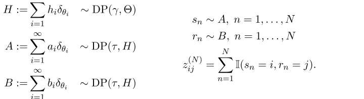
andB. To ensure the two distributions have the same support (meaning that any node can have both incoming and outgoing links), we couple these two distributions via a shared, discrete base measureH. The generalized process becomes
H:=
∞
X
i=1
hiδθi ∼DP(γ,Θ)
A:=
∞
X
i=1
aiδθi ∼DP(τ, H)
B:=
∞
X
i=1
biδθi ∼DP(τ, H)
sn∼A, n= 1, . . . , N
rn∼B, n= 1, . . . , N
z(Nij )=
N
X
n=1
I(sn=i, rn=j).
(4)
Figure 2b shows a network constructed in this manner; note the nodes that “send” a large number of links are not necessarily those that “receiver” a large number of links. The concentration parameter τ governs how similar the two distributions are to the base measure, and hence to each other.
sender, this tells us nothing about the receiver. This makes it a poor model for real-world networks, where we observe cliques of users who are strongly interconnected, or groups that interact with other groups in characterizable manners. While we cannot capture such behavior with the basic symmetric or asymmetric Dirichlet network distributions described above, we can use them as a component of more complex and flexible models.
3.2 Mixtures of Dirichlet Network Distributions
Rather than use a single Dirichlet network distribution over integer-valued networks, as described by Equations 2 and 4, we can use a mixture of such distributions, which we will refer to as a mixture of Dirichlet network distributions, or MDND. By ensuring both sender and receiver belong to a common mixture component, we break the independence between sender and receiver, allowing us to identify communication patterns that cannot be captured using the DND or the related Caron and Fox (2015) model.. To allow links between the subgraphs associated with each mixture component, we couple the networks using a shared, discrete base measureH. Concretely, in the asymmetric case, let
D:=(dk, k∈N) ∼GEM(α)
H :=
∞
X
i=1
hiδθi ∼DP(γ,Θ)
Ak:= ∞
X
i=1
ak,iδθi ∼DP(τ, H), k= 1,2, . . .
Bk:=
∞
X
i=1
bk,iδθi ∼DP(τ, H)
cn∼D, n= 1, . . . , N sn∼Acn
rn∼Bcn
z(Nij )=
N
X
n=1
I(sn=i, rn=j),
(5)
where GEM(α) is the distribution over the size-biased atom sizes of a Dirichlet process with concentration parameterα. Figure 2c shows a network constructed in this manner. A symmetric version of the MDND is recovered if we replace the sender- and receiver-specific distributions Ak and Bk with a shared distribution Gk ∼ DP(τ, H), and is appropriate when we believe the distribution over edges originating from a given node is similar to the distribution over edges ending at that node. For the remainder of this paper, we will focus on the asymmetric setting.
We can verbalize the generative process of the asymmetric MDND as follows. To gener-ate thenth link, we first select a cluster cn. We then select a “sender” sn and a “receiver” rn—identifying a link (sn, rn)—according to the cluster-specific distributionsAcn and Bcn. The concentration parameters α,τ and γ can be manipulated to obtain differing network properties. The parameterα controls the number of clusters, with the total number of clus-ters used to modelN links growing approximately asO(γlogN). The parameterτ controls the degree of similarity between the clusters: Asτ decreases, the overlap between clusters will tend to decrease. Increasingγ increases the overall number of nodes represented in the network.
is no specific ordering of the links, or where the order is believed to be irrelevant. This has useful implications for inference: It means we can easily construct a Gibbs sampler, as described in Section 4. However, in many networks the order in which links are formed does carry information. In Section 3.3, we discuss an extension for explicitly ordered binary links, and in Section 6, we will discuss possible extensions of the integer-valued network model to explicitly ordered links.
3.3 Extension: Binary-valued Networks
Many real-world networks exhibit binary, rather than real-valued, edges. One way of cap-turing this behavior is to threshold the integer-valued edges generated by the DND or the MDND. The most straightforward version of this is simply to sample a networkZ = (zij) according to the DND or the MDND, and then generate a binary network Y = (yij) by lettingyij = 1 iffzij >0. If we place a negative binomial distribution overN =Pi,jzij, so
thatN ∼NB(α,1/(1 +β)) for someβ >0, we can represent this thresholded model as
Γ :=
∞
X
k=1
µkδθk ∼GP(αD0, β)
G0 ∼DP(γ, H0)
Gk ∼DP(τ, G0), k= 1,2, . . . Nk ∼Poisson(µk)
N :=X
k Nk
s(k)n ∼Gk, n= 1, . . . , Nk rn(k)∼Gk
zij(N)=
∞
X
k=1 Nk
X
n=1
I(s(k)n =i, rn(k) =j) y(Nij )=I(zij(N) >0),
(6)
where GP indicates a gamma process. This approach is a form of restricted exchangeable distribution, as described by Williamson et al. (2013). As in the unrestricted, integer-valued network, the distribution over edge events is exchangeable. We note that this truncation technique is the same as that used by Caron and Fox (2015) to generate binary networks, and indeed ifZ is the symmetric version of the DND given by Equation 3, and if we obtain a symmetric network by mirroring the link counts, then this construction corresponds to the binary network described in Caron and Fox (2015), itself a special case of the class of binary network models described by Veitch and Roy (2015).
If our observations are explicitly ordered, and we believe that ordering to be important, we can modify the DND or the MDND to sample without replacement from the set of possible links, giving a non-exchangeable model. This form of non-exchangeability mimics behavior found in many naturally-occurring networks. For example, in a social network, a user will add their close friends first, and then over time add more distant acquaintances. In integer-valued networks exchangeability can represent the fact that close friends will communicate both early and often, but in an exchangeable binary setting all relationships appear identical.
D:=(dk, k∈N) ∼GEM(α)
H :=
∞
X
i=1
hiδθi ∼DP(γ,Θ)
Ak:=
∞
X
i=1
ak,iδθi ∼DP(τ, H), k = 1,2, . . .
Bk:= ∞
X
i=1
bk,iδθi ∼DP(τ, H)
ct∼D, t= 1,2, . . .
st∼Act
rt∼Bct
yij(t)=I
t X
t0=1
I(st0 =i, rt0 =j)>0
.
Due to the finite probability of sampling an existing (s, r) pair, Y(t+1) may be the
same asY(t); instead we would likely work with the corresponding non-repeating sequence (Z(n), n ∈N), where Z(n) = mint0
Y(t0) :Pt0
t=1I(Yt 6=Yt−1) =n
. While this censored
model is no longer exchangeable, we can make use of the underlying exchangeable sequence of interactions to make predictions.
3.4 Relationship to Other Models
As we described in Section 3.1, the Dirichlet network distribution is strongly related to the sparse network models of Caron and Fox (2015)—in fact, conditioned on the total number of links, the integer-valued model of Caron and Fox (2015) is a special case of the symmetric DND, and the truncated model of Equation 6 describes the binary model of Caron and Fox (2015) as a special case. However, the DND on its own lacks the flexibility to model structured networks, where nodes tend to belong to locally connected sub-networks, and where knowing who sent a message tells us something about the intended recipient. The mixture of Dirichlet network distributions allows us to capture multiple sub-networks, while allowing interaction between sub-networks via a common Dirichlet process-distributed base measure H.
A related integer-valued network model is described by Crane and Dempsey (2016). This model is explicitly designed for multi-way interactions, such as collaborations or actors co-starring in movies, but can be modified to give two-way interactions. The number of “roles” in an interaction is sampled from an appropriate distribution, and for each role, nodes are sampled from a (single) Pitman-Yor process. The two-way interaction setting corresponds to a Pitman-Yor variant of the symmetric Dirichlet network distribution obtained by replacing the Dirichlet process in Equation 2 with a Pitman-Yor process; as such it is unable to capture the clustering behavior obtained using the mixture of Dirichlet network distributions.
representation. For the mixture models proposed in Sections 3.2 and 3.3, the predictive distribution depends on the values of latent variables, but we can easily sample from this distribution, as we will see in Section 4.
While the MDND does not explicitly cluster the nodes, we can obtain a similar mixed-membership interpretation to that found in the MMSB. We can think of each cluster of links representing a latent topic of conversation between nodes. Each topic of conversation is described by distributions over the nodes likely to take part in such a conversation. If we condition on the fact that the sth node is sending an email, we can use these distributions to infer the probability of that email belonging to a given discussion. Since the hierarchical construction of Equation 5 ensures that the topics of conversation have overlapping par-ticipants, the node will be associated with a conditional distribution over an unbounded number of conversations.
In Section 2.2, we discussed how the graphex construction for binary exchangeable net-works by Veitch and Roy (2015) allows us to represent the stochastic blockmodel and the sparse binary model of Caron and Fox (2015) using a common framework. While the integer-valued MDND, and the non-exchangeable binary network described in Section 3.3, do not fall under the graphex framework, it suggests an alternative way to describe the ex-changeable binary network obtained by thresholding a MDND (as described in Equation 6).
4. Fully Nonparametric Inference via an Urn Scheme
In the simple symmetric network model of Equation 2, we can directly evaluate the pre-dictive distribution over the nth link, given the previousn−1 links, via a straightforward extension of the P¨olya urn sampler for the Chinese restaurant process Neal (1998), where the probability of seeing a link between two nodes is proportional to the product of those nodes’ degrees (excluding the link in question):
P(yn= (s, r)|y1, . . . , yn−1) =
mi(mj+I(i=j))
(2n−2+τ)(2n−1+τ) ifmi 6= 0, mj 6= 0 miτ
(2n−2+τ)(2n−1+τ) ifmi 6= 0, mj = 0 mjτ
(2n−2+τ)(2n−1+τ) ifmi = 0, mj 6= 0 τ1+I(i=j)
(2n−2+τ)(2n−1+τ) ifmi = 0, mj = 0,
wheremi=Pn−1
n0=1(I(sn0 =i) +I(rn0 =i)) is the sum of the links to or from nodei.
The MDND is based on a mixture of coupled hierarchical Dirichlet processes, allowing us to construct a collapsed Gibbs sampler by modifying the direct assignment sampler for the hierarchical Dirichlet process introduced by Teh et al. (2006). Recall that associated with each cluster kwe have a sender-specific distribution Ak and a receiver-specific distribution
Bk.1 Letηk=
PN
i=1Ici=k be the number of links associated with clusterk; let m
(1)
k,i be the
number of edges associated with cluster kthat originate from node i(that is, edges where nodeiis the “sender”); and let m(2)k,i be the number of edges associated with clusterkthat end at node i (that is, edges where node i is the “receiver”). We also introduce auxiliary
count variablesρ(1)k,i andρ(2)k,i2and a probability vector (β1, . . . , βJ, βu)∼Dir(ρ(·1·), . . . , ρ(·J·), γ), whereρ··i=P
kρ (1) k,i+ρ
(2)
k,i; hereβ1, . . . , βJ correspond to the atoms ofHthat are associated
with represented nodes, and βu =P∞
j=J+1hj.
The distribution over the cluster assignment of the nth link, givenβ and all otherN−1 links, is given by:
P(cn=k|sn, rn, c¬n, β)∝
(
η¬kn(m(1)k,s¬n
n +τ βsn)(m
(2)¬n
k,rn +τ βrn) ifη
¬n k >0 ατ2β
snβrn ifη
¬n k = 0.
(7)
where we use c¬n to indicate the sequence (cn0 :n0 6=n) and m(1)¬n
k,i =
P
n06=nIc
n0=k,sn0=i, i.e., the¬nnotation is used to exclude the value associated with the current observation.
Following Fox et al. (2007) we can sample the “dish counts” ρ(1)k,i (ρ(2)k,i) by simulating the partitioning of m(1)k,i (m(2)k,i) according to a Chinese restaurant process with parameter
τ βk.
Conditioned on the cluster assignments for the first N links, and the probability vector (β1, . . . , βJ, βu), we can evaluate the predictive distribution over theN + 1st link as:
P(yN+1= (s, r)|c1:N, y1:N, β) =
PK+ k=1 ηk N+α
m(1)k,s+τ βs
ηk+τ
m(2)k,r+τ βr
ηk+τ +
α
N+αβsβr ifs, r ≤J
PK+
k=1 ηk
N+α
m(1)k,s+τ βs
ηk+τ βu+
α
N+αβsβu ifs≤J, r > J
PK+
k=1 ηk
N+αβu
m(2)k,r+τ βr
ηk+τ +
α
N+αβuβr ifr ≤J, s > J
βu2 ifr, s > J.
To improve mixing, we augmented the sampler with split/merge moves, proposed using the Restricted Gibbs method of Jain and Neal (2004).
5. Experimental Evaluation
We begin by demonstrating the ability of the MDND to recover latent network structure in a two synthetically-generated data sets, before performing a quantitative analysis on three real-world networks.
5.1 Synthetic Data
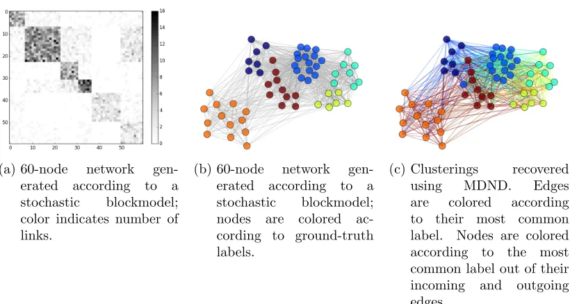
In Figure 3, we show the performance of the MDND evaluated on a 60-node network generated according to a stochastic blockmodel. A distribution over cluster memberships was drawn from a Dirichlet(5,5,5,5,5,5) distribution. Intra-cluster link parameters θi,i
were distributed according to θi,i ∼ Gamma(5,1), and inter-cluster link parameters θi,j
were distributed according to θi,j ∼ Gamma(0.5,1). Link counts zsr for each pair (s, r) were Poisson-distributed given the appropriate parameter θcs,cr, where cs is the cluster of
2. In the Chinese franchise interpretation of Teh et al. (2006),ρ(1)k,i andρ
(2)
k,i correspond to the number of
(a) 60-node network gen-erated according to a stochastic blockmodel; color indicates number of links.
(b) 60-node network gen-erated according to a stochastic blockmodel; nodes are colored ac-cording to ground-truth labels.
(c) Clusterings recovered
using MDND. Edges
are colored according to their most common label. Nodes are colored according to the most common label out of their incoming and outgoing edges.
Figure 3: Structure recovery: stochastic blockmodel.
node s. The raw matrix of link counts is shown in Figure 3a, and a visualization of the matrix is shown in Figure 3b, where the edge color indicates the number of nodes and the node color indicates the ground-truth cluster labels.3
Figure 3c shows the structure recovered by the MDND. Each edge in the MDND repre-sentation has multiple cluster labels, one per link; the edges are colored according to their most common cluster label. The nodes are colored according to the most common cluster label amongst their incoming and outgoing edges. As we can see from Figure 3c, all but one node is most commonly associated with its ground-truth label.
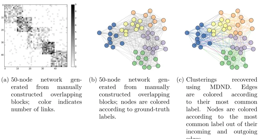
Figure 4 evaluates the MDND on a 50-node with manually constructed overlapping blocks. The network shown in Figure 4a was generated from 5 equiprobable clusters; each cluster puts 95% of its probability mass on one of five overlapping blocks, and the remaining mass is uniformly distributed over the entire population. Figure 4b shows a visualization of this matrix, where the edge color indicates the number of nodes and the node color indicates most common ground-truth label amongst the incoming and outgoing edges, as in Figure 3b. Figure 4c shows the structure recovered by the MDND; as before, the edges are colored according to their most common cluster label, and the nodes are colored according to the most common cluster label amongst their incoming and outgoing edges. Again, we have very high agreement between the ground-truth labels and the recovered clustering.
5.2 Real Network Data
We compared the mixture of Dirichlet network distributions to the infinite relational model, the mixed membership stochastic blockmodel, and several baselines, in three real-world scenarios: A small network representing character interactions in Shakespeare’s ‘Macbeth’;
(a) 50-node network gen-erated from manually constructed overlapping blocks; color indicates number of links.
(b) 50-node network gen-erated from manually constructed overlapping blocks; nodes are colored according to ground-truth labels.
(c) Clusterings recovered
using MDND. Edges
are colored according to their most common label. Nodes are colored according to the most common label out of their incoming and outgoing edges.
Figure 4: Structure recovery: Overlapping blocks.
a medium-sized network representing political interactions; and a large network representing email interactions. In Section 5.2.1 we describe the comparison methods, and in Section 5.2.2 we describe the three networks and present our results.
5.2.1 Comparison Methods
We compare the mixture of Dirichlet network distributions to a single symmetric Dirichlet network distribution; to integer-valued variants of the mixed-membership stochastic block-model (MMSB, Airoldi et al., 2008) and the infinite relational block-model (IRM, Kemp et al., 2006); and to two baseline methods.
1. Symmetric Dirichlet network distribution. We modeled the data using a single symmetric DND as described in Section 3.1, with Dirichlet process concentration parameterτ = 1.
2. Infinite relational model. Kemp et al. (2006) describe a variant of the IRM ap-propriate for integer-valued data. Each pair of clusters (i, j) is associated with a positive real-valued parameter θij, and the N links are assigned to clusters
accord-ing to a multinomial distribution parametrized by the θij. Inference in this model is
performed using existing C code released by the authors of Kemp et al. (2006). This code was not able to handle the number of nodes present in the Enron data sets.
extension. We perform inference in this model, with K = 50 clusters, using Gibbs sampling, via an existing R package (Chang, 2012) that was modified to replace the beta/Bernoulli pairs with gamma/Poisson pairs. Since inference in this model was significantly slower than inference in the IRM and the DNM, we only compared with the gamma/Poisson MMSB on our smallest data set.
4. Baseline 1: equiprobable links. Our first baseline assumed that all (sender, re-ceiver) pairs are equally likely, provided the sender and receiver are different—so if we have M nodes, the probability of a given link is 1/M(M −1).
5. Baseline 2: Dirichlet-multinomial distribution over links. Here we assumed an M(M−1)-dimensional Dirichlet prior over the potential links, and looked at the conditional distribution given the N observed links,
P((sN+1, rN+1) = (i, j)) =
PN
n=1I(sn=i, rn=j) +αij M(M−1) +N .
We note that this corresponds to an IRM where each pair of nodes is in its own cluster.
5.2.2 Evaluation on Three Real Networks
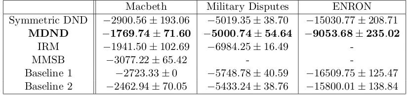
We compared the mixture of Dirichlet network distributions to the comparison methods de-scribed above, on three real data sets. We describe the data sets below; Table 1 summarizes the networks’ statistics.
1. Macbeth. This data set represents the implied social network in Shakespeare’s ‘Mac-beth’. We constructed a directed network where each link indicates an uninterrupted block of speech from the speaker to all other characters presently on stage. To evaluate predictive performance, we split the play into 5 contiguous subsets, each containing (approximately) N/5 consecutive edges. We used these subsets to generate a 5-fold split into training data (4 of the 5 subsets) and a test set (the remaining one subset), and evaluated the joint predictive likelihood on the test set.
2. Militarized disputes. Next, we evaluated our model on a network representing militarized disputes between 188 countries (Maoz, 2005). The data set contains 8650 disputes between 1816 and 1976. We split this data set into 10 subsets, and used these subsets to generate 10 train/test splits, where 9 subsets were used for training and 1 for evaluation.
3. ENRON email network. Finally, we looked at subsets of the ENRON email data set (Klimmt and Yang, 2004). We looked at five training sets, corresponding to the total set of emails sent and received in each of the first 5 months of 2000. For each data set, we evaluated predictive performance on the first 1000 emails sent in the subsequent month.
Network Number of links (N) Number of nodes (M) N/M2
Macbeth 2153 39 1.42
Military Disputes 8650 188 0.245
Enron (average) 13994 3883.8 9.14e-4
Enron (range) 8692–20464 3006–4652 7.55e-4–1.03e-3
Table 1: Network statistics. Note that the Macbeth and Military Disputes data sets were split into equally sized subsets, while the Enron data set was split according to month. We therefore report both the average and the range of the Enron monthly statistics.
Macbeth Military Disputes ENRON
Symmetric DND −2900.56±193.06 −5019.35±38.70 −15030.77±208.71
MDND −1769.74±71.60 −5000.74±54.64 −9053.68±235.02
IRM −1941.50±102.69 −6984.25±16.49
-MMSB −3077.22±65.42 -
-Baseline 1 −2723.33±0 −5748.78±40.59 −16509.75±125.47 Baseline 2 −2462.94±70.05 −5433.24±38.76 −15800.01±138.84
Table 2: Test set log likelihood (mean ±standard error).
set explicitly included those nodes with interactions present in the test set but not in the training set. We note that this is an unrealistic setting that gives an advantage to the MMSB and the IRM: In most situations, the number of new nodes is unknown. However, without including at least the correct number of unseen nodes, we would be unable to obtain an estimate for the predictive performance on the data sets used.
For the IRM and the MMSB, we already have cluster assignments for each pair of nodes, and can use the cluster parameters to directly obtain a probability distribution over pairs of nodes. We use this probability distribution to directly calculate the joint predictive log likelihood. For the MDND, we do not yet have cluster assignments for the test set links. It is analytically intractable to sum over all possible test set cluster assignments. Instead, we estimate the predictive log likelihood using our Gibbs sampler to generate 100 samples of the test cluster assignments, conditioned on the training set assignments and the test set links. We then use the harmonic mean of the likelihoods given these cluster assignments as an estimator for the overall joint predictive likelihoods.
The MMSB code was unable to run on the Disputes and ENRON data sets, and the IRM code was unable to run on the ENRON data set. By looking at the ratio M/N2
We see that, in each case, the MDND out-performs the comparison methods—even though we have included more information in the MMSB and the IRM by making use of the number of unseen nodes.
6. Discussion and Future Work
We have presented a new Bayesian nonparametric model, the mixture of Dirichlet network distributions, for integer-valued networks where the number of nodes is unbounded and grows in expectation with the number of binary links. This model allows us to capture sparse networks with latent structure. Existing network models focus either on latent structure—capturing the fact that each node will have a different pattern over which nodes it connects with—or on capturing sparsity; this is, to our knowledge, the first model that combines these two goals. Further, unlike most existing Bayesian network models, this model is explicitly designed for prediction. We can use the mixture of Dirichlet network distributions to obtain an explicit predictive distribution over the nodes associated with an as-yet unseen observation, even if we have not observed these nodes in our training set; we have shown good predictive and qualitative performance on a variety of data sets.
The mixture of Dirichlet network distributions is based on a simpler network model that we refer to as a Dirichlet network distribution. In the symmetric setting—where a common distribution is used for both senders and receivers—this corresponds to a special case of the integer-valued network models of Caron and Fox (2015) and Crane and Dempsey (2016). While these models can be used to obtain desirable properties such as network sparsity and power law degree distribution, they are unable to capture community-type structure in the network. By using a mixture of these networks, we can capture multiple modalities of interaction between nodes; by using a nonparametric hierarchical framework we ensure that both the number of nodes is unbounded, and that nodes can interact as part of multiple clusters. The MDND therefore increases the modeling flexibility of this class of models, while retaining desirable sparsity properties.
The mixture of Dirichlet network distributions is an exchangeable model: It is invari-ant to permutations of the order in which we observe links. While this is computationally appealing and leads to a straightforward predictive distribution, it does not allow us to capture network dynamics in integer-valued networks. In practice, such dynamics may be important: an individual’s level of activity within a topic may vary over time, and the over-all popularity of topics may change. A number of authors have found that adding temporal dynamics to network models improves performance (Ishiguro et al., 2010; Xing et al., 2010; Xu and Hero III, 2013). In the case of Dirichlet network distributions, similar temporal dy-namics could be incorporated by replacing some or all of the component Dirichlet processes with dependent Dirichlet processes (MacEachern, 2000; Lin et al., 2010; Ren et al., 2008); we intend to explore this in a future work.
than the integer-valued case. While we can analytically sample the censored observations as auxiliary variables and recover the integer network, the number of censored observations grows according to a coupon-collector problem with the number of observed links, making this approach infeasible for large data sets. An interesting avenue for future research is to develop scalable inference methods for this setting.
Acknowledgments
Sinead Williamson is supported by NSF grant 1447721.
References
E.M. Airoldi, D.M. Blei, S.E. Fienberg, and E.P. Xing. Mixed membership stochastic blockmodels. Journal of Machine Learning Research, 9:1981–2014, 2008.
A.A. Amini, A. Chen, P.J. Bickel, and E. Levina. Pseudo-likelihood methods for community detection in large sparse networks. The Annals of Statistics, 41(4):2097–2122, 2013.
A. Brix. Generalized gamma measures and shot-noise Cox processes. Advances in Applied Probability, 31(4):929–953, 1999.
F. Caron and E.B. Fox. Sparse graphs using exchangeable random measures. arXiv:1401.1137 [stat.ME], 2015.
J. Chang. lda: Collapsed Gibbs sampling methods for topic models., 2012. URL http:
//CRAN.R-project.org/package=lda. R package version 1.3.2.
H. Crane and W. Dempsey. Edge exchangeable models for network data. arXiv:1603.04571 [math.ST], 2016.
E.B. Fox, E.B. Sudderth, M.I. Jordan, and A.S. Willsky. The sticky HDP-HMM: Bayesian nonparametric hidden Markov models with persistent states. Technical Report P-2777, Massachusetts Institute of Technology, 2007.
Q. Ho, J. Yin, and E.P. Xing. On triangular versus edge representations—towards scalable modeling of networks. In Advances in Neural Information Processing Systems (NIPS), pages 2132–2140, 2012.
P.W. Holland, K.B. Laskey, and S. Leinhardt. Stochastic blockmodels: First steps. Social networks, 5(2):109–137, 1983.
K. Ishiguro, T. Iwata, N. Ueda, and J.B. Tenenbaum. Dynamic infinite relational model for time-varying relational data analysis. In Advances in Neural Information Processing Systems (NIPS), pages 919–927, 2010.
C. Kemp, J.B. Tenenbaum, T.L. Griffiths, T. Yamada, and N. Ueda. Learning systems of concepts with an infinite relational model. In National Conference on Artificial Intelli-gence (AAAI), pages 381–388, 2006.
B. Klimmt and Y. Yang. Introducing the Enron corpus. In Conference on Email and Anti-Spam (CEAS), 2004.
A. Lijoi, I. Pr¨unster, and S.G. Walker. Investigating nonparametric priors with Gibbs structure. Statistica Sinica, 18(4):1653–1668, 2008.
D. Lin, E. Grimson, and J.W. Fisher III. Construction of dependent Dirichlet processes based on Poisson processes. In Advances in Neural Information Processing Systems (NIPS), pages 1396–1404, 2010.
J. Lloyd, P. Orbanz, Z. Ghahramani, and D.M. Roy. Random function priors for ex-changeable arrays with applications to graphs and relational data. InAdvances in Neural Information Processing Systems (NIPS), pages 1007–1015, 2012.
S.N. MacEachern. Dependent Dirichlet processes. Unpublished manuscript, Department of Statistics, The Ohio State University, 2000.
Z. Maoz. Dyadic militarized interstate dispute dataset, version 2.0. http://psfaculty.ucdavis.edu/zmaoz/dyadmid.html, 2005.
M. Mariadassou, S. Robin, and C. Vacher. Uncovering latent structure in valued graphs: A variational approach. Annals of Applied Statistics, 4(2):715–742, 2010.
R.M. Neal. Markov chain sampling methods for Dirichlet process mixture models. Technical Report 9815, Dept. of Statistics, University of Toronto, 1998.
P. Orbanz and D. Roy. Bayesian models of graphs, arrays and other exchangeable random structures. IEEE Transactions on Pattern Analysis and Machine Intelligence, 37(2): 437–461, 2014.
J. Pitman and M. Yor. The two-parameter Poisson-Dirichlet distribution derived from a stable subordinator. The Annals of Probability, 25(2):855–900, 1997.
L. Ren, D.B. Dunson, and L. Carin. The dynamic hierarchical Dirichlet process. In Inter-national Conference on Machine Learning (ICML), pages 824–831, 2008.
T.A.B. Snijders and T. Nowicki. Estimation and prediction for stochastic blockmodels for graphs with latent block structure. Journal of Classification, 14(1):75–100, 1997.
Y.W. Teh, M.I. Jordan, M.J. Beal, and D.M. Blei. Hierarchical Dirichlet processes. Journal of the American Statistical Association, 101(476):1566–1581, 2006.
V. Veitch and D. Roy. The class of random graphs arising from exchangeable random measures. arXiv:1512.03099 [math.ST], 2015.
Y.J. Wang and G.Y. Wong. Stochastic blockmodels for directed graphs. Journal of the American Statistical Association, 82(397):8–19, 1987.
S.A. Williamson, S.N. MacEachern, and E.P. Xing. Restricting nonparametric distributions. In Advances in Neural Information Processing Systems (NIPS), pages 2598–2606, 2013.
E.P. Xing, W. Fu, and L. Song. A state-space mixed membership blockmodel for dynamic network tomography. The Annals of Applied Statistics, 4(2):535–566, 2010.