Learning Minimum Volume Sets
Clayton D. Scott [email protected]
Department of Statistics Rice University
Houston, TX 77005, USA
Robert D. Nowak [email protected]
Department of Electrical and Computer Engineering University of Wisconsin at Madison
Madison, WI 53706, USA
Editor: John Lafferty
Abstract
Given a probability measure P and a reference measure µ, one is often interested in the minimum µ-measure set with P-measure at leastα. Minimum volume sets of this type summarize the regions of greatest probability mass of P, and are useful for detecting anomalies and constructing confi-dence regions. This paper addresses the problem of estimating minimum volume sets based on independent samples distributed according to P. Other than these samples, no other information is available regarding P, but the reference measure µ is assumed to be known. We introduce rules for estimating minimum volume sets that parallel the empirical risk minimization and structural risk minimization principles in classification. As in classification, we show that the performances of our estimators are controlled by the rate of uniform convergence of empirical to true probabilities over the class from which the estimator is drawn. Thus we obtain finite sample size performance bounds in terms of VC dimension and related quantities. We also demonstrate strong universal consistency, an oracle inequality, and rates of convergence. The proposed estimators are illustrated with histogram and decision tree set estimation rules.
Keywords: minimum volume sets, anomaly detection, statistical learning theory, uniform
devia-tion bounds, sample complexity, universal consistency
1. Introduction
Given a probability measure P and a reference measure µ, the minimum volume set (MV-set) with mass at least 0<α<1 is
G∗α=arg min{µ(G): P(G)≥α,G measurable}.
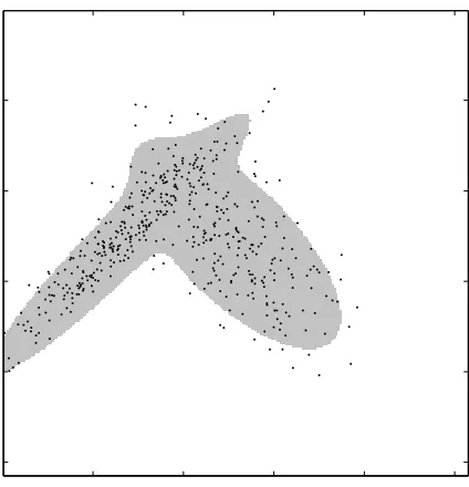
MV-sets summarize regions where the mass of P is most concentrated. For example, if P is a mul-tivariate Gaussian distribution and µ is the Lebesgue measure, then the MV-sets are ellipsoids. An MV-set for a two-component Gaussian mixture is illustrated in Figure 1. Applications of minimum volume sets include outlier/anomaly detection, determining highest posterior density or multivari-ate confidence regions, tests for multimodality, and clustering. See Polonik (1997); Walther (1997); Sch¨olkopf et al. (2001) and references therein for additional applications.
Figure 1: Minimum volume set (gray region) of a two-component Gaussian mixture. Also shown are 500 points drawn independently from this distribution.
the estimation process are the significance level α, the reference measure µ, and a collection of candidate sets
G
.A major theme of this work is the strong parallel between MV-set estimation and binary classi-fication. In particular, we find that uniform convergence (of true probability to empirical probability over the class of sets
G
) plays a central role in controlling the performance of MV-set estimators. Thus, we derive distribution free finite sample performance bounds in terms of familiar quantities such as VC dimension. In fact, as we will see, any uniform convergence bound can be directly converted to a rule for MV-set estimation.1.1 Previous Work
All previous theoretical work on MV-set estimation has been asymptotic in nature, to our knowl-edge. Our work here is the first to provide explicit finite sample bounds. Most closely related to this paper is the pioneering work of Polonik (1997). Using empirical process theory, he establishes con-sistency results and rates of convergence for minimum volume sets which depend on the entropy of the class of candidate sets. This places restrictions on the MV-set G∗α (e.g, µ(G∗α) is continu-ous inα), whereas our consistency result holds universally, i.e., for all distributions P. Also, the convergence rates obtained by Polonik apply under smoothness assumptions on the density. In con-trast, our rate of convergence results in Section 6 depend on the smoothness of the boundary of G∗α. Walther (1997) studies an approach based on “granulometric smoothing,” which involves applying certain morphological smoothing operations to theα-mass level set of a kernel density estimate. His rates also apply under smoothness assumptions on the density, rather than more direct assumptions regarding the smoothness of the MV-set as in our approach.
Algorithms for MV-set estimation have been developed for convex sets (Sager, 1979) and el-lipsoidal sets (Hartigan, 1987) in two dimensions. Unfortunately, for more complicated problems (dimension>2 and non-convex sets), there has been a disparity between practical MV-set estima-tors and theoretical results. Polonik (1997) makes no comment on the practicality of his estimaestima-tors. The smoothing estimators of Walther (1997) in practice must approximate the theoretical estima-tor via iterative level set estimation. On the other hand, computationally efficient procedures like those in Sch¨olkopf et al. (2001) and Huo and Lu (2004) are motivated by the minimum volume set paradigm, but their performance relative to G∗α is not known. Recently, however, Mu˜noz and Moguerza (2006) have proposed the so-called one-class neighbor machine and demonstrated its consistency under certain assumptions. Our proposed algorithms for histograms and decision trees are practical in low dimensional settings, but appear to be constrained by the same computational limitations as empirical risk minimization in binary classification.
More broadly, MV-set estimation theory has similarities (in terms of the nature of results and technical devices) to other set estimation problems, such as classification, discrimination analysis, density support estimation (which corresponds to the caseα=1), and density level set estimation, to which we now turn.
1.2 Connection to Density Level Sets
specified, while density level sets are not. Further advantages of MV-sets over level sets are given in the concluding section.
Algorithms for density level set estimation can be split into two categories, implicit plug-in methods and explicit set estimation methods. Plug-in strategies entail full density estimation and are the more popular practical approach. For example, Baillo et al. (2001) considers plug-in rules for density level set estimation problems and establishes upper bounds on the rate of convergence for such estimators in certain cases. The problem of estimating a density support set, the zero level set, is a special minimum volume set (i.e., the minimum volume set that contains the total probability mass). Cuevas and Fraiman (1997) study density support estimation and show that a certain (density estimator) plug-in scheme provides universally consistent support estimation.
While consistency and rate of convergence results for plug-in methods typically make global smoothness assumptions on the density, explicit methods make assumptions on the density at or near the level of interest. This fact, together with the intuitive appeal of not having to solve a problem harder than one is interested in, make explicit methods attractive. Steinwart et al. (2005) reduce level set estimation to a cost-sensitive classification problem by sampling from the reference measure. The idea of sampling from µ in the minimum volume context is discussed further in the concluding section. Vert and Vert (2005) study the one-class support vector machine (SVM) and show that it produces a consistent density level set estimator, based on the fact that consistent density estimators produce consistent plug-in level set estimators. Willett and Nowak (2005, 2006) propose a level set estimator based on decision trees, which is applicable to density level set estimation as well as regression level set estimation, and related dyadic partitioning schemes are developed by Klemel¨a (2004) to estimate the support set of a density.
The connections between MV-sets and density level sets will be important later in this paper. To make the connection precise the following assumption on the data-generating distribution and reference measure is needed. We emphasize that this assumption is not necessary for the results in Sections 2 and 3, where distribution free error bounds and universal consistency are established.
A1 P has a density f with respect to µ.
A key result relating density level and MV-sets is the following, stated without proof (see, e.g., Nunez-Garcia et al. (2003)).
Lemma 1 Under assumption A1 there existsγαsuch that for any MV-set G∗α,
{x : f(x)>γα} ⊂G∗α⊂ {x : f(x)≥γα}.
Note that every density level set is an MV-set, but not conversely. If, however, µ({x : f(x) =γα}) = 0, then the three sets in the Lemma coincide.
1.3 Notation
Let(
X
,B
)be a measure space withX
⊂Rd. Let X be a random variable taking values inX
with distribution P. Let S= (X1, . . . ,Xn) be an independent and identically distributed (IID) sampledrawn according to P. Let G denote a subset of
X
, and letG
be a collection of such subsets. LetPb denote the empirical measure based on S:b
P(G) = 1 n
n
∑
i=1Here I(·) is the indicator function. The notation µ will denote a measure1 on
X
. Denote by f the density of P with respect to µ (when it exists), γ>0 a level of the density, andα∈(0,1) a user-specified mass constraint. Defineµ∗α=inf
G {µ(G): P(G)≥α}, (1)
where the inf is over all measurable sets. A minimum volume set, G∗α, is a minimizer of (1) when it exists.
2. Minimum Volume Sets and Empirical Risk Minimization
We introduce a procedure inspired by the empirical risk minimization (ERM) principle for classifi-cation. In classification, ERM selects a classifier from a fixed set of classifiers by minimizing the empirical error (risk) of a training sample. Vapnik and Chervonenkis established the basic theoret-ical properties of ERM (see Vapnik, 1998; Devroye et al., 1996), and we find similar properties in the minimum volume setting.
Let
G
be a class of sets. Givenα∈(0,1), denoteG
α = {G∈G
: P(G)≥α},the collection of all sets in
G
with mass at leastα. DefineµG,α=inf{µ(G): G∈
G
α} (2)and
GG,α=arg min{µ(G): G∈
G
α} (3)when it exists. Thus GG,αis the best approximation to the minimum volume set G∗αfrom
G
.Empirical versions of
G
αand GG,αare defined as follows. Letφ(G,S,δ)be a function of G∈G
,the training sample S, and a confidence parameterδ∈(0,1). Set
b
G
α={G∈G
:P(G)b ≥α−φ(G,S,δ)}and
b
GG,α=arg min{µ(G): G∈
G
bα}. (4)We refer to the rule in (4) as MV-ERM because of the analogy with empirical risk minimization in classification. A discussion of the existence and uniqueness of the above quantities is deferred to Section 2.5.
The quantityφacts as a kind of “tolerance” by which the empirical mass may deviate from the targeted valueα. Throughout this paper we assume thatφsatisfies the following.
Definition 2 We sayφis a (distribution free) complexity penalty for
G
if and only if for all distri-butions P and allδ∈(0,1),Pn
(
S : sup
G∈G
P(G)−P(G)b −φ(G,S,δ)>0
)! ≤δ.
Thus,φcontrols the rate of uniform convergence ofP(G)b to P(G)for G∈
G
. It is well known that the performance of ERM (for binary classification) relative to the performance of the best classifier in the given class is controlled by the uniform convergence of true to empirical probabilities. A similar result holds for MV-ERM.Theorem 3 Ifφis a complexity penalty for
G
, then PnP(GbG,α)<α−2φ(GbG,α,S,δ)
orµ(GbG,α)>µG,α
≤δ.
Proof Consider the sets
ΘP = {S : P(GbG,α)<α−2φ(GbG,α,S,δ)},
Θµ = {S : µ(GbG,α)>µ(GG,α)},
ΩP = (
S : sup
G∈G
P(G)−P(G)b −φ(G,S,δ)>0
)
.
Lemma 4 WithΘP,Θµ, andΩPas defined above we have ΘP∪Θµ⊂ΩP.
The proof is given in Appendix A, and follows closely the proof of Lemma 1 in Cannon et al. (2002). The theorem statement follows directly from this observation.
Lemma 4 may be understood by analogy with the result from classification that says
R
(bf)− inff∈FR
(f)≤2 supf∈F |R
(f)−R
b(f)| (see Devroye et al. (1996), Ch. 8). HereR
andR
b are the true and empirical risks, bf is the empirical risk minimizer, andF
is a set of classifiers. Just as this result relates uniform convergence to empirical risk minimization in classification, so does Lemma 4 relate uniform convergence to the performance of MV-ERM.The theorem above allows direct translation of uniform convergence results into performance guarantees on MV-ERM. Fortunately, many penalties (uniform convergence results) are known. In the next two subsections we take a closer look at penalties for VC classes and countable classes, and a Rademacher penalty.
2.1 Example: VC Classes
Let
G
be a class of sets with VC dimension V , and defineφ(G,S,δ) =
r
32V log n+log(8/δ)
n . (5)
By a version of the VC inequality (Devroye et al., 1996), we know thatφis a complexity penalty for
G
, and therefore Theorem 3 applies.To view this result in perhaps a more recognizable way, let ε>0 and choose δ such that
Corollary 5 With the notation defined above, Pn
P(GbG,α)<α−2ε
or
µ(GbG,α)>µG,α
≤8nVe−nε2/128.
Thus, for any fixedε>0, the probability of being within 2εof the target massαand being less than the target volume µG,αapproaches one exponentially fast as the sample size increases. This result
may also be used to calculate a distribution free upper bound on the sample size needed to be within a given toleranceεofαand with a given confidence 1−δ. In particular, the sample size will grow no faster than a polynomial in 1/εand 1/δ, paralleling results for classification.
2.2 Example: Countable Classes
Suppose
G
is a countable class of sets. Assume that to every G∈G
a numberJGKis assigned such that∑
G∈G2−JGK≤1. (6)
In light of the Kraft inequality for prefix2codes (Cover and Thomas, 1991),JGKmay be defined as the codelength of a codeword for G in a prefix code for
G
. Letδ>0 and defineφ(G,S,δ) =
r
JGKlog 2+log(2/δ)
2n . (7)
By Chernoff’s bound together with the union bound, φis a penalty for
G
. Therefore Theorem 3 applies and we have a result analogous to the Occam’s Razor bound for classification (see Langford, 2005).As a special case, suppose
G
is finite and takeJGK=log2|G
|. Settingε=φ(G,S,δ)and invert-ing the relationship betweenδandε, we have the following.Corollary 6 For the MV-ERM estimateGbG,αfrom a finite class
G
Pn
P(GbG,α)<α−2ε
or
µ(GbG,α)>µG,α
≤2|
G
|e−nε2/2.As with VC classes, these inequalities may be used for sample size calculations.
2.3 The Rademacher Penalty for Sets
The Rademacher penalty was originally studied in the context of classification by Koltchinskii (2001) and Bartlett et al. (2002). For a succinct exposition of its basic properties, see Bousquet et al. (2004). An analogous penalty exists for sets. Letσ1, . . . ,σnbe Rademacher random variables,
i.e., independent random variables taking on the values 1 and -1 with equal probability. Denote
b
P(σi)(G) =1n∑ n
i=1σiI(Xi∈G). We define the Rademacher average
ρ(
G
) =E"
sup
G∈G
b
P(σi)(G)
#
and the conditional Rademacher average
b
ρ(
G
,S) =E(σi)"
sup
G∈G
b
P(σi)(G)
#
,
where the second expectation is with respect the Rademacher random variables only, and condi-tioned on the sample S.
Proposition 7 With probability at least 1−δover the draw of S,
P(G)−P(G)b ≤2ρ(
G
) +r
log(1/δ) 2n
for all G∈
G
. With probability at least 1−δover the draw of S,P(G)−P(G)b ≤2bρ(
G
,S) +r
2 log(2/δ) n
for all G∈
G
.The proof of this result follows exactly the same lines as the proof of Theorem 5 in Bousquet et al. (2004), and is omitted.
Assume
G
satisfies the property that G∈G
⇒G∈G
, where G denotes the compliment of G. Then P(G)b −P(G) =P(G)−P(G), and so the upper bounds of Proposition 7 also apply tob|P(G)−P(G)b |. Thus we are able to define the conditional Rademacher penalty
φ(G,S,δ) =2bρ(
G
,S) +r
2 log(2/δ) n .
By the above Proposition, this is a complexity penalty according to Definition 2. The conditional Rademacher penalty is studied further in Section 7 and in Appendix E, where it is shown thatbρ(
G
,S) can be computed efficiently for sets based on a fixed partition ofX
(such as histograms and trees).2.4 Comparison to Generalized Quantile Processes Polonik (1997) studies the empirical quantile function
b
Vα=inf{µ(G):P(G)b ≥α},
and the MV-set estimate that achieves the minimum (when it exists). The only difference compared with MV-ERM is the absence of the termφ(G,S,δ)in the constraint. Thus, MV-ERM will tend to produce estimates with smaller volume and smaller mass. While Polonik proves only asymptotic properties of his estimator, we have demonstrated finite sample bounds for MV-ERM. Moreover, in Section 5, we show that the results of this section extend to a generalization of MV-ERM where
2.5 Existence and Uniqueness
In this section we discuss the existence and uniqueness of the sets GG,αandGbG,α. Regarding the
former, it is really not necessary that a minimizer exist. All of our results are stated in terms of µG,α,
which certainly exists. When a minimizer exists, its uniqueness is not an issue for the same reason. Our results above involve only µG,α, which is the same regardless of which minimizer is chosen.
Yet one may wonder whether convergence of the volume and mass to their optimal values implies convergence to the MV-set (when it is unique) in any sense. A result in this direction is presented in Theorem 10 below.
For the MV-ERM estimateGbG,α, uniqueness is again not an issue because all results hold even
if the minimizer is chosen arbitrarily. As for existence, we must be more careful. We cannot make the same argument as for GG,αbecause we are ultimately interested in a concrete set estimate, not
just its volume and mass. Clearly, if
G
is finite,GbG,αexists. For more general sets, existence mustbe examined on a case-by-case basis. For example, if
X
⊂Rd, µ is the Lebesgue measure, andG
is the VC class of spherical or ellipsoidal sets, thenGbG,αcan be seen to exist.In the event thatGbG,αdoes not exist, it suffices to letGbG,αbe a set whose volume comes within
εof the infimum, whereεis arbitrarily small. Then our results still hold with µ(GbG,α)replaced by
µ(GbG,α)−ε. The consistency and rate of convergence results below are unchanged, as we may take
ε→0 arbitrarily fast as a function of n.
3. Consistency
A minimum volume set estimator is consistent if its volume and mass tend to the optimal values µ∗α andαas n→∞. Formally, define the error quantity
E
(G):= (µ(G)−µ∗α)++ (α−P(G))+,where(x)+=max(x,0). We are interested in MV-set estimators such that
E
(GbG,α)tends to zero asn→∞.
Definition 8 A learning ruleGbG,αis strongly consistent if
lim
n→∞
E
(GbG,α) =0 with probability 1.IfGbG,αis strongly consistent for every possible distribution of X , thenGbG,αis strongly universally
consistent.
In this section we show that if the approximating power of
G
increases in a certain way as a function of n, then MV-ERM leads to a universally consistent learning rule.To see how consistency might result from MV-ERM, it helps to rewrite Theorem 3 as follows. Let
G
be fixed and letφ(G,S,δ)be a penalty forG
. Then with probability at least 1−δ, bothµ(GbG,α)−µ∗α≤µ(GG,α)−µ∗α (8)
and
hold. We refer to the left-hand side of (8) as the excess volume of the class
G
and the left-hand side of (9) as the missing mass ofGbG,α. The upper bounds on the right-hand sides are an approximationerror and a stochastic error, respectively.
The idea is to let
G
grow with n so that both errors tend to zero as n→∞. IfG
does not change with n, universal consistency is impossible. Either the approximation error will be nonzero for most distributions (whenG
is too small) or the bound on the stochastic error will be too large (otherwise). For example, if a class has universal approximation capabilities, its VC dimension is necessarily infinite (Devroye et al., 1996, Ch. 18).To have both stochastic and approximation errors tend to zero, we apply MV-ERM to a class
G
k from a sequence of classesG
1,G
2, . . ., where k=k(n)grows with the sample size. Given such a sequence, defineb
GGk,α = arg min{µ(G): G∈
G
bαk}, (10)where
b
G
αk ={G∈G
k:P(G)b ≥α−φk(G,S,δ)}andφk is a penalty for
G
k.Theorem 9 Choose k=k(n)andδ=δ(n)such that 1. k(n)→∞as n→∞
2. ∑∞n=1δ(n)<∞
Assume the sequence of sets
G
kand penaltiesφk satisfy
lim
k→∞Ginf∈Gk
α
µ(G) =µ∗α (11)
and
lim
n→∞Gsup∈Gk
φk(G,S,δ(n)) =0. (12)
ThenGbGk,αis strongly universally consistent.
The proof is given in Appendix B. We now give some examples that satisfy these conditions.
3.1 Example: Hierarchy of VC Classes
Assume
G
1,G
2, . . . ,is a family of VC classes with VC dimensions V1<V2< . . . .For G∈G
kdefine φk(G,S,δ) =r
32Vklog n+log(8/δ)
n . (13)
By takingδ(n)≍n−β for some β>1 and k such that Vk =o(n/log n)the assumption in (12) is
3.2 Example: Histograms
Assume
X
= [0,1]d, and letG
kbe the class of all sets formed by taking unions of cells in a regularpartition of
X
into hypercubes of sidelength 1/k. EachG
khas 2kdmembers and we may therefore apply the penalty for finite sets discussed in Section 2.2. To satisfy the Kraft inequality (6) it suffices to takeJGK=kd. The penalty for G∈
G
kis thenφk(G,S,δ) = r
kdlog 2+log(2/δ)
2n . (14)
By takingδ(n)≍n−β for some β>1 and k such that kd=o(n) the assumption in (12) is satis-fied. The assumption in (11) is satisfied by the well-known universal approximation capabilities of histograms. Thus the conditions for consistency of histograms for minimum volume set estimation are exactly parallel to the conditions for consistency of histogram rules for classification (Devroye et al., 1996, Ch. 9). Dyadic decision trees, discussed below in Section 6, are another countable family for which consistency results are possible.
3.3 The Symmetric Difference Performance Metric
An alternative measure of performance for an MV-set estimator is the µ-measure of the symmetric difference, µ(GbG,α∆G∗α), where A∆B= (A\B)∪(B\A). Although this performance metric has been
commonly adopted in the study of density level sets, it is less desirable for our purposes. First, unlike with density level sets, there may not be a unique MV-set (imagine the case where the density of P has a plateau). Second, as pointed out by Steinwart et al. (2005), there is no known way to estimate the accuracy of this measure using only samples from P. Nonetheless, the symmetric difference metric coincides asymptotically with our error metric
E
in the sense of the following result. The theorem uses the notationγαto denote the density level corresponding to the MV-set, as discussed in Section 1.2.Theorem 10 Assume µ is a probability measure and P has a density f with respect to µ. Let Gn denote a sequence of sets. If G∗α is a minimum volume set and µ(Gn∆G∗α)→0 with n, then
E
(Gn)→0. Conversely, assume µ({x : f(x) =γα}) =0. IfE
(Gn)→0, then µ(Gn∆G∗α)→0.The proof is given in Appendix C. The assumption of the second part of the theorem ensures that G∗α is unique, otherwise the converse statement need not be true. The proof of the converse reveals yet another connection between MV-set estimation and classification. In particular, we show that
E
(Gn) bounds the excess classification risk for a certain classification problem. Theconverse statement then follows from a result of Steinwart et al. (2005) who show that this excess classification risk and the µ-measure of the symmetric difference tend to zero simultaneously.
4. Structural Risk Minimization and an Oracle Inequality
The results of this and subsequent sections are no longer distribution free. In particular, we assume
A1 P has a density f with respect to µ.
A2 for allα′∈(0,1), G∗α′ exists and P(G∗α′) =α′.
Note that A2 holds if f has no plateaus, i.e., µ({x : f(x) =γ}) =0 for allγ>0. This is a commonly made assumption in the study of density level sets. However, A2 is somewhat more general. It still holds, for example, if µ is absolutely continuous with respect to Lebesgue measure, even if f has plateaus.
Recall from Section 1.2 that under assumption A1, there existsγα>0 such for any MV-set G∗α,
{x : f(x)>γα} ⊂G∗α⊂ {x : f(x)≥γα}.
Let
G
be a class of sets. Intuitively, viewG
as a collection of sets of varying capacities, such as a union of VC classes or a union of finite classes (examples are given below). Letφ(G,S,δ)be a penalty forG
. The MV-SRM principle selects the setb
GG,α = arg min
G∈G
n
µ(G) +2φ(G,S,δ):P(G)b ≥α−φ(G,S,δ)o. (15)
Note that MV-SRM is different from MV-ERM because it minimizes a complexity penalized vol-ume instead of simply the volvol-ume. We have the following oracle inequality for MV-SRM. Recall
E
(G):= (µ(G)−µ∗α)++ (α−P(G))+.Theorem 11 LetGbG,αbe the MV-set estimator in (15) and assume A1 and A2 hold. With
proba-bility at least 1−δover the training sample S,
E
(GbG,α)≤
1+ 1
γα
inf
G∈Gα
µ(G)−µ∗α+2φ(G,S,δ)
. (16)
Although the value of 1/γαis in practice unknown, it can be bounded by
1
γα≤
µ(
X
)−µ∗α 1−α ≤µ(
X
) 1−α.This follows from the bound 1−α≤γα·(µ(
X
)−µ∗α)on the mass outside the minimum volume set. If µ is a probability measure, then 1/γα≤1/(1−α).The oracle inequality says that MV-SRM performs about as well as the set chosen by an oracle to optimize the tradeoff between excess volume and missing mass.
4.1 Example: Union of VC Classes Consider
G
=∪Kk=1
G
k, whereG
k has VC dimension Vk, V1<V2<···, and K is possibly infinite.A penalty for
G
can be obtained by defining, for G∈G
k,φ(G,S,δ) =φk(G,S,δ2−k),
whereφk is the penalty from Equation (13). Then φis a penalty for
G
becauseφk is a penalty forG
k, and by applying the union bound and the fact∑selects an MV-set estimate from a VC class that balances approximation and stochastic errors. Note that instead of settingδk=δ2−k one could also chooseδk∝k−β,β>1.
To be more concrete, suppose
G
kis the collection of sets whose boundaries are defined bypoly-nomials of degree k. It may happen that for certain distributions, the MV-set is well-approximated by a quadratic region (such as an ellipse), while for other distributions a higher degree polynomial is required. If the appropriate polynomial degree for the MV-set is not known in advance, as would be the case in practice, then MV-SRM adaptively chooses an estimator of a certain degree that does about as well as if the best degree was known in advance.
4.2 Example: Union of Histograms Let
G
=∪Kk=1
G
k, whereG
kis as in Section 3.2. As with VC classes, we obtain a penalty forG
by defining, for G∈G
k,φ(G,S,δ) =φk(G,S,δ2−k),
whereφkis the penalty from Equation (14). Then MV-SRM adaptively chooses a partition resolution
k that approximates the MV-set about as well as possible without overfitting the training data. This example is studied experimentally in Section 7.
5. Damping the Penalty
In Theorem 3, the reader may have noticed that MV-ERM does not equitably balance the excess volume (µ(GbG,α)relative to its optimal value) with the missing mass (P(GbG,α)relative toα). Indeed,
with high probability, µ(GbG,α)is less than µ(GG,α), while P(GbG,α)is only guaranteed to be within
2φ(GbG,α) ofα. The net effect is that MV-ERM (and MV-SRM) underestimates the MV-set. Our
experiments in Section 7 demonstrate this to be the case.
In this section we introduce variants of MV-ERM and MV-SRM that allow the total error to be shared between the volume and mass, instead of all of the error residing in the mass term. Our approach is to introduce a damping factor−1≤ν≤1 that scales the penalty. We will see that the resulting MV-set estimators obey performance guarantees like those we have already seen, but with the total error redistributed between the volume and mass. The reason for not introducing this more general framework initially is that the results are slightly less general, more involved to state, and to some extent follow as corollaries to the original (ν=1) framework.
The extensions of this section encompass the generalized quantile estimate of Polonik (1997), which corresponds toν=0. Thus we have finite sample size guarantees for that estimator to match Polonik’s asymptotic analysis. The caseν=−1 is also of interest. If it is crucial that the estimate satisfies the mass constraint P(GbG,α)≥α(note that this involves the true probability measure P),
settingν=−1 ensures this to be the case with probability at least 1−δ.
First we consider damping the penalty in MV-ERM. Assume that the penalty is independent of G∈
G
and of the sample S, although it can depend on n andδ. That is,φ(G,S,δ) =φ(n,δ). For example,φmay be the penalty in (5) for VC classes or (7) for finite classes. Letν≤1 and defineb
GνG,α=arg min
G∈G
n
Sinceφis independent of G∈
G
,GbνG,αcoincides with the MV-ERM estimate (as originallyformu-lated)GbG,α′ but at the adjusted mass constraintα′=α+ (1−ν)φ(n,δ). Therefore, we may apply Theorem 3 to obtain the following.
Corollary 12 Letα′=α+ (1−ν)φ(n,δ). Then Pn
P(GbνG,α)<α−(1+ν)φ(n,δ)or
µ(GbG,α)>µG,α′)
≤δ.
Relative to the original formulation of MV-ERM, the bound on the missing mass is decreased by a factor(1+ν). On the other hand, the volume is now bounded by µG,α′=µG,α+ (µG,α′−µG,α). Thus the bound on the excess volume is increased from 0 to µG,α′−µG,α. This may be interpreted as a stochastic component of the excess volume. Relative to the MV-set, µ(GbG,α) has only an
approximation error, whereas µ(GbνG,α)has both approximation and stochastic errors. The advantage is that now the stochastic error of the mass is decreased.
A similar construction applies to MV-SRM. Now assume
G
=∪Kk=1
G
k. Given a scale parameterν, define
b
GνG,α=arg min
G∈G
n
µ(G) + (1+ν)φ(G,S,δ):P(G)b ≥α−νφ(G,S,δ)o.
As above, assume φ is independent of the sample and constant on each
G
k. Denote εk(n,δ) = φ(G,S,δ) for G∈G
k. Observe that computing GbνG,α is equivalent to computing the MV-ERM
estimate on each
G
k at the levelα(k,ν) =α+ (1−ν)εk(n,δ), and then minimizing the penalized
volume over these MV-ERM estimates.
Like the original MV-SRM, this modified procedure also obeys an oracle inequality. Recall the notation
G
kα(k,ν)={G∈
G
k: P(G)≥α(k,ν)}={G∈G
k: P(G)≥α+ (1−ν)εk(n,δ)}.Theorem 13 Let−1≤ν≤1. Setα(k,ν) =α+ (1−ν)εk(n,δ). Assume A1 and A2 hold. With
probability at least 1−δ,
E
(GbνG,α)≤
1+ 1
γα
min 1≤k≤K
"
inf
G∈Gk
α(k,ν)
n
µ(G)−µ∗α(k,ν)o+Ckεk(n,δ) #
, (17)
where Ck=
(1+ν) + 1
γα(k,ν)(1−ν)
.
Hereγα(k,ν)is the density level corresponding to the MV-set with massα(k,ν). It may be bounded above in terms of known quantities, as discussed in the previous section. The proof of the theorem is very similar to the proof of the earlier oracle inequality and is omitted, although it may be found in Scott and Nowak (2005a). Notice that in the caseν=1 we recover Theorem 11 (under the stated assumptions on
G
andφ). Also note thatG
αk(k,ν)will be empty ifα(k,ν)>1, in which case those k should be excluded from the min.To understand the result, assume that the rate at which
G
kαapproximates G∗αis independent ofα.
In other words, the rate at which infG∈Gk
αµ(G)−µ∗αtends to zero as k increases is the same for allα.
Then in the theorem we may replace the expression infG∈Gk
α(k,ν)µ(G)−µ ∗
α(k,ν)with infG∈Gk
αµ(G)−µ∗α.
penalty by νhas the effect of decreasing the stochastic mass error and adding a stochastic error to the volume. This follows from the above discussion of MV-ERM and the observation that the MV-SRM coincides with an MV-SRM estimate over
G
k for some k. The improved balancing ofvolume and mass error is confirmed by our experiments in Section 7.
6. Rates of Convergence for Tree-Structured Set Estimators
In this section we illustrate the application of MV-SRM, when combined with an appropriate anal-ysis of the approximation error, to the study of rates of convergence. To preview the main result of this section (Theorem 16), we will consider the class of distributions such that the decision bound-ary has Lipschitz smoothness (loosely speaking) and d′ of the d features are relevant. The best rate of convergence for this class is n−1/d′. We will show that MV-SRM can achieve this rate (within a log factor) without knowing d′or which features are relevant. This demonstrates the strength of the oracle inequality, from which the result is derived.
To obtain these rates we apply MV-SRM to sets based on a special family of decision trees called dyadic decision trees (DDTs) (Scott and Nowak, 2006). Before introducing DDTs, however, we first introduce the class of distributions
D
with which our study is concerned. Throughout this section we assumeX
= [0,1]dand µ is the Lebesgue (equivalently, uniform) measure.Somewhat related to the approach considered here is the work of Klemel¨a (2004) who consid-ers the problem of estimating the support of a uniform density. The estimators proposed therein are based on dyadic partitioning schemes similar in spirit to the DDTs studied here. However, it is important to point out that in the support set estimation problem studied by Klemel¨a (2004) the boundary of the set corresponds to discontinuity of the density, and therefore more standard complexity-regularization and tree pruning methods commonly employed in regression settings suf-fice to achieve near minimax rates. In contrast, DDT methods are capable of attaining near minimax rates for all density level sets whose boundaries belong to certain H¨older smoothness classes, regard-less of whether or not there is a discontinuity at the given level. Significantly different risk bounding and pruning techniques are required for this additional capability (Scott and Nowak, 2006).
6.1 The Box-Counting Class
Before introducing
D
we need some additional notation. Let m denote a positive integer, and defineP
m to be the collection of md cells formed by the regular partition of[0,1]d into hypercubes ofsidelength 1/m. Let c1,c2>0 be positive real numbers. Let G∗αbe a minimum volume set, assumed to exist, and let∂G∗αbe the topological boundary of G∗α. Finally, let Nm(∂G∗α)denote the number of
cells in
P
mthat intersect∂G∗α.We define the box-counting class to be the set
D
BOX=D
BOX(c1,c2)of all distributions satisfying A1’ : X has a density f with respect to µ and f is essentially bounded by c1.A3 :∃G∗αsuch that Nm(∂G∗α)≤c2md−1for all m.
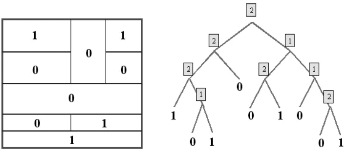
Figure 2: A dyadic decision tree (right) with the associated recursive dyadic partition (left) in d=2 dimensions. Each internal node of the tree is labeled with an integer from 1 to d indicating the coordinate being split at that node. The leaf nodes are decorated with class labels.
of convergence to be n−1/d(the typical rate for set estimation problems characterized by Lipschitz smoothness). See Scott and Nowak (2006) for further discussion of the box-counting assumption.
6.2 Dyadic Decision Trees
Let T denote a tree structured classifier T :[0,1]d→ {0,1}. Each such T gives rise to a set G T = {x∈[0,1]d: T(x) =1}. In this subsection we introduce a certain class of trees, and later consider
MV-SRM over the induced class of sets.
Scott and Nowak (2006) demonstrate that dyadic decision trees (DDTs) offer a computationally feasible classifier that also achieves optimal rates of convergence (for standard classification) under a wide range of conditions. DDTs are especially well suited for rate of convergence studies. Indeed, bounding the approximation error is handled by the restriction to dyadic splits, which allows us to take advantage of recent insights from multiresolution analysis and nonlinear approximations (DeVore, 1998; Cohen et al., 2001; Donoho, 1999). An analysis similar to that of Scott and Nowak (2006) applies to MV-SRM for DDTs, leading to similar results: optimal rates of convergence for a computationally efficient learning algorithm.
A dyadic decision tree is a decision tree that divides the input space by means of axis-orthogonal dyadic splits. More precisely, a DDT T is a binary tree (with a distinguished root node) specified by assigning (1) an integer c(v)∈ {1, . . . ,d} to each internal node v of T (corresponding to the coordinate that gets split at that node); (2) a binary label 0 or 1 to each leaf node of T . The nodes of DDTs correspond to hyperrectangles (cells) in[0,1]d. Given a hyperrectangle A=∏d
c=1[ac,bc],
let Ac,1and Ac,2 denote the hyperrectangles formed by splitting A at its midpoint along coordinate c. Specifically, define Ac,1={x∈A|xc≤(ac+bc)/2}and Ac,2=A\Ac,1.
Each node of T is associated with a cell according to the following rules: (1) The root node is associated with[0,1]d; (2) If v is an internal node associated with the cell A, then the children of v are
associated with Ac(v),1and Ac(v),2. See Figure 2. Note that every T corresponds to a set GT∈[0,1]d
Let L=L(n)be a natural number and define
T
Lto be the collection of all DDTs such that (1) noleaf cell has a sidelength smaller than 2−L, and (2) any two leaf nodes that are siblings have different labels. Condition (1) says that when traversing a path from the root to a leaf no coordinate is split more than L times. Condition (2) means that it is impossible to “prune” at any internal node and still have the same set/classifier. Also define
A
L to be the collection of all cells A that correspondto nodes of DDTs in
T
L. Defineπ(T)to be the collection of “leaf” cells of T . For a cell A∈A
L,let j(A) denote the depth of A when viewed as a node in some DDT. Observe that when µ is the Lebesgue measure, µ(A) =2−j(A).
6.3 MV-SRM with Dyadic Decision Trees We study MV-SRM over the family
G
L={GT : T ∈
T
L}, where L is set by the user. To simplifythe notation, at times we will suppress the dependence ofφon the training sample S and confidence parameterδ. Thus our MV set estimator has the form
b
Gα=arg min
G∈GL
n
µ(G) +2φ(G)|P(G) +b φ(G)≥αo. (18)
It remains to specify the penaltyφ. There are a number of ways to produceφsatisfying
Pn
(
S : sup
G∈GL
P(G)−P(G)b −φ(G,S,δ)>0
)! ≤δ.
Since
G
Lis countable (in fact, finite), one approach is to devise a prefix code forG
Land apply thepenalty in Section 2.2. Instead, we employ a different penalty which has the advantage that it leads to minimax optimal rates of convergence. Introduce the notationJAK= (3+log2d)j(A), which may be thought of as the codelength of A in a prefix code for
A
L, and define the minimax penaltyφ(GT):=
∑
A∈π(T)s
8 max
b
P(A),JAKlog 2+log(2/δ)
n
JAKlog 2+log(2/δ)
n . (19)
For each A∈π(T), setℓ(A) =1 if A⊂GT and 0 otherwise. The bound originates from writing
P(GT)−P(Gb T) =
∑
A∈π(T):ℓ(A)=1P(A)−P(A)b
and
b
P(GT)−P(GT) = P(GT)−P(Gb T)
=
∑
A∈π(T):ℓ(A)=0
P(A)−P(A)b
from which it follows that
|P(GT)−P(Gb T)| ≤
∑
A∈π(T)P(A)−P(A)b . (20)
There are many ways to do this (additive Chernoff, relative Chernoff, exact tail inversion, etc.), but the one we have chosen is particularly convenient for rate of convergence analysis. For further discussion, see Scott and Nowak (2006). Proof of the following result is nearly identical to a similar result in Scott and Nowak (2006), and is omitted.
Proposition 14 Letφbe as in (19) and letδ∈(0,1). With probability at least 1−δover the draw of S,
|P(G)−P(G)b | ≤φ(G) for all G∈
G
L. Thusφis a complexity penalty forG
L.The MV-SRM procedure over
G
Lwith the above penalty leads to an optimal rate of convergencefor the box-counting class.
Theorem 15 Choose L=L(n)andδ=δ(n)such that 1. 2L(n)<(n/log n)1/d
2. δ(n) =O(plog n/n)and log(1/δ(n)) =O(log n)
DefineGbαas in (18) withφas in (19). For d≥2 we have
sup DBOX
En
E
(Gbα)4
log n n
1
d
. (21)
We omit the proof, since this theorem is a special case of Theorem 16 below. Note that the condition onδis satisfied ifδ(n)≍n−βfor someβ>1/2.
6.4 Adapting to Relevant Features
The previous result could have been obtained without using MV-SRM. Instead, we could have applied MV-ERM to a fixed hierarchy
G
L(1),G
L(2), . . .where L(n)≍(n/log n)1/d. The strength ofMV-SRM and the associated oracle inequality is in its ability to adapt to favorable conditions on the data generating distribution which may not be known in advance. Here we illustrate this idea when the number of relevant features is not known in advance.
We define the relevant data dimension to be the number d′≤d of relevant features. A feature Xi, i=1, . . . ,d, is said to be relevant provided f(X)is not constant when Xi is varied from 0 to 1. For example, if d=2 and d′=1, then∂G∗αis a horizontal or vertical line segment (or union of such line segments). If d=3 and d′=1, then∂G∗αis a plane (or union of planes) orthogonal to one of the axes. If d=3 and the third coordinate is irrelevant (d′=2), then∂G∗αis a “vertical sheet” over a curve in the(X1,X2)plane (see Figure 3).
Let
D
BOX′ =D
BOX′ (c1,c2,d′) be the set of all product measures Pn such that A1’ and A3 hold
for the underlying distribution P, and X has relevant data dimension d′≥2. An argument of Scott and Nowak (2006) implies that the expected minimax rate for d′relevant features is n−1/d′. By the following result, MV-SRM can achieve this rate to within a log factor.
Figure 3: Cartoon illustrating relevant data dimension. If the X3axis is irrelevant, then the boundary of the MV-set is a “vertical sheet” over a curve in the(X1,X2)plane.
2. δ(n) =O(plog n/n)and log(1/δ(n)) =O(log n)
DefineGbαas in (18) withφas in (19). If d′≥2 then
sup D′
BOX
En
E
(Gbα)4
log n n
1
d′
. (22)
The proof hinges on the oracle inequality. The details of the proof are very similar to the proof of a result in Scott and Nowak (2006) and are therefore omitted. Here we just give a sketch of how the oracle inequality comes into play.
Let K ≤L and let G∗K ∈
G
Kα be such that (i) µ(G∗K) =arg minG∈GK
αµ(G)−µ∗α; and (ii) G∗K is
based on the smallest possible partition among all sets satisfying (i). Set m=2K. It can be shown that
µ(G∗K)−µ∗α+φ(G∗K,S,δ)4m−1+md′/2−1
r
log n n
in expectation. This upper bound is minimized when m≍(n/log n)1/d′, in which case we obtain
the stated rate. Here the oracle inequality is crucial because m depends on d′, which is not known in advance. The oracle inequality tells us that MV-SRM performs as if it knew the optimal K.
Note that the set estimation rule does not require knowledge of the constants c1 and c2, nor d′, nor which features are relevant. Thus the rule is completely automatic and adaptive.
7. Experiments
In this section we conduct some simple numerical experiments to illustrate the rules for MV-set estimation proposed in this work. Our objective is not an extensive comparison with competing methods, but rather to demonstrate that our estimators behave in a way that agrees with the the-ory, to gain insight into the behavior of various penalties, and to examine basic algorithmic issues. Throughout this section we take
X
= [0,1]dand µ to be the Lebesgue (equivalently, uniform)7.1 Histograms
We devised a simple numerical experiment to illustrate MV-SRM in the case of histograms (see Sections 3.2 and 4.2). In this case, MV-SRM can be implemented exactly with a simple procedure. First, compute the MV-ERM estimate for each
G
k, k=1, . . . ,K, where 1/k is the bin-width. To dothis, for each k, sort the cells of the partition according to the number of samples in the cell. Then, begin incorporating cells into the estimate one cell at a time, starting with the most populated, until the empirical mass constraint is satisfied. Finally, once all MV-ERM estimates have been computed, choose the one that minimizes the penalized volume.
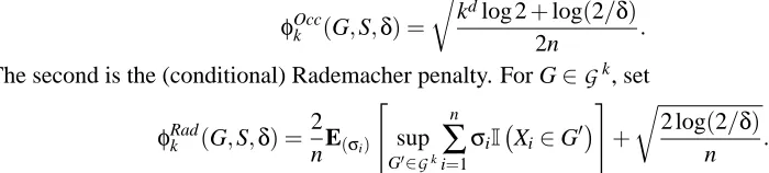
We consider two penalties. Both penalties are defined viaφ(G,S,δ) =φk(G,S,δ2−k)for G∈
G
k,whereφk is a penalty for
G
k. The first is based on the simple Occam-style bound of Section 3.2.For G∈
G
k, setφOcc
k (G,S,δ) = r
kdlog 2+log(2/δ)
2n .
The second is the (conditional) Rademacher penalty. For G∈
G
k, setφRad
k (G,S,δ) =
2 nE(σi)
"
sup
G′∈Gk
n
∑
i=1σiI Xi∈G′
#
+
r
2 log(2/δ) n .
Hereσ1, . . . ,σnare Rademacher random variables, i.e., independent random variables taking on the
values 1 and -1 with equal probability. Fortunately, the conditional expectation with respect to these variables can be evaluated exactly in the case of partition-based rules such as the histogram. See Appendix E for details.
As a data set we consider
X
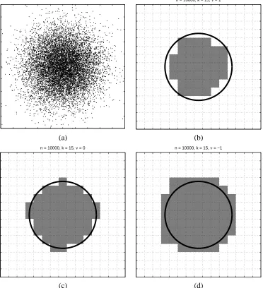
= [0,1]d, the unit square, and data generated by a two-dimensionaltruncated Gaussian distribution, centered at the point(1/2,1/2)and having spherical variance with parameterσ=0.15. Other parameter settings areα=0.8, K=40, andδ=0.05. All experiments were conducted at nine different sample sizes, logarithmically spaced from 100 to 1000000, and repeated 100 times. Figure 4 shows a representative training sample and MV-ERM estimates with
ν=1,0, and−1. These examples clearly demonstrate that the largerν, the smaller the estimate. Figure 5 depicts the error
E
(G)b of the MV-SRM estimate with ν=1. The Occam’s Razor penalty consistently outperforms the Rademacher penalty. For comparison, a damped version (ν= 0) was also evaluated. It is clear from the graphs thatν=0 outperformsν=1. This happens because the damped version distributes the error more evenly between mass and volume, as discussed in Section 5.Figure 6 depicts the penalized volume of the MV-ERM estimates (ν=1) as a function of the resolution k, where 1/k is the sidelength of the histogram cell. MV-SRM selects the resolution where this curve is minimized. Clearly the Occam’s Razor bound is tighter than the Rademacher bound (look at the right side of the graph), which explains why Occam outperforms Rademacher. Figure 7 depicts the average resolution of the estimate (top) and the average symmetric difference with respect to the true MV-set, for various sample sizes. These graphs are forν=1. The graphs forν=0 do not change considerably. Thus, while damping seems to have a noticeable effect on the error quantity
E
, the effect on the symmetric difference is much less pronounced.7.2 Dyadic Decision Trees
n = 10000, k = 15, ν = 1
(a) (b)
n = 10000, k = 15, ν = 0 n = 10000, k = 15, ν = −1
(c) (d)
100 1000 10000 100000 1000000 0
0.05 0.1 0.15 0.2 0.25 0.3 0.35 0.4 0.45 0.5
net error as a function of sample size
occam rademacher
100 1000 10000 100000 1000000
0 0.02 0.04 0.06 0.08 0.1 0.12
net error as a function of sample size
occam rademacher
Figure 5: The error
E
(GbG,α)as a function of sample size for the histogram experiments in Section0 5 10 15 20 25 30 35 40 0.4
0.5 0.6 0.7 0.8 0.9 1 1.1
resolution parameter k
average penalized volume of MV−ERM solution
10000 samples
occam rademacher
100 1000 10000 100000 1000000 2
4 6 8 10 12 14
sample size
average resolution (1/binwidth) of mv−srm estimate
occam rademacher
100 1000 10000 100000 1000000
0.05 0.1 0.15 0.2 0.25 0.3 0.35 0.4
symmetric difference as a function of sample size
occam rademacher
algorithm based on a reformulation of the constrained optimization problem defining MV-SRM in terms of its Lagrangian, coupled with a bisection search to find the appropriate Lagrange multiplier. If the penalty is additive, then the unconstrained Lagrangian can be minimized efficiently using existing algorithmic approaches.
A penalty for a DDT is said to be additive if it can be written in the form
φ(GT) =
∑
A∈π(T)ψ(A)
for someψ. Ifφis additive the optimization in (18) can be re-written as
min
T∈TL
∑
A∈π(T)
[µ(A)ℓ(A) + (1+ν)ψ(A)] subject to
∑
A∈π(T)
h b
P(A)ℓ(A) +νψ(A)i≥α
whereℓ(A)is the binary label of leaf A (ℓ(A) =1 if A is in the candidate set and 0 otherwise). In-troducing the Lagrange multiplierλ>0, the unconstrained Lagrangian formulation of the problem is
min
T A
∑
∈T h
µ(A)ℓ(A) + (1+ν)ψ(A)−λP(A)b ℓ(A) +νψ(A)i.
Inspection of the Lagrangian reveals that the optimal choice ofℓ(A)is
ℓ(A) =
1 ifλP(A)b ≥µ(A),
0 otherwise
Thus, we have a “per-leaf” cost function
cost(A) :=min(µ(A)−λP(A)b ,0) + (1+ν(1−λ))ψ(A)
For a given value ofλ, the optimal tree can be efficiently obtained using the algorithm of Blanchard et al. (2004).
We also note that the above strategy works for tree structures besides the one studied in Section 6. For example, suppose an overfitted tree (with arbitrary, non-dyadic splits) has been constructed by some greedy heuristic (perhaps using an independent data set). Or, suppose that instead of binary dyadic splits with arbitrary orientation, one only considers “quadsplits” whereby every parent node has 2d children (in fact, this is the tree structure used for our experiments below). In such cases, optimizing the Lagrangian reduces to a classical pruning problem, and the optimal tree can be found by a simple O(n)dynamic program that has been used since at least the days of CART (Breiman et al., 1984).
LetTbλdenote the tree resulting from the Lagrangian optimization above. From standard opti-mization theory, we know that for each value ofλ,Tbλwill coincide withGbα, for a certain value of
α. For each value ofλthere is a correspondingα, but the converse is not necessarily true. There-fore, the Lagrangian solutions correspond to many, but not all possible solutions of the original MV-SRM optimization with different values ofα. Despite this potential limitation, the simplicity of the Lagrangian optimization makes this a very attractive approach to MV-SRM in this case. We can determine the best value ofλfor a given targetαby repeatedly solving the Lagrangian optimization and finding the setting forλthat meets or comes closest to the original constraint. The search over
In our experiments we do not consider the “free-split” tree structure described in Section 6, in which each parent has two children defined by one of d=2 possible splits. Instead, we assume a quadsplit tree structure, whereby every cell is a square, and every parent has four square children. The total optimization time is O(mn), where m is the number of steps in the bisection search. In our experiments presented below we found that ten steps (i.e., ten Lagrangian tree pruning optimiza-tions) were sufficient to meet the constraint almost exactly (whenever possible).
We consider three complexity penalties. We refer to the first penalty as the minimax penalty, since it is inspired by the minimax optimal penalty in (19):
ψmm(A):= (0.01) s
8 max
b
P(A),JAKlog 2+log(2/δ)
n
JAKlog 2+log(2/δ)
n . (23)
Note that the penalty is down-weighted by a constant factor of 0.01, since otherwise it is too large to yield meaningful results:3
The second penalty is based on the Rademacher penalty (see Section 2.3). LetΠLdenote the set of all partitions πof trees in
T
L. Givenπ0 ∈ΠL, set
G
π0 ={GT ∈G
L:π(T) =π
0}. Recall
π(T)denotes the partition associated with the tree T . Combining Proposition 7 with the results of Appendix E, we know that for any fixedπ,
∑
A∈πs b
P(A) n +
r
2 log(2/δ) n
is a complexity penalty for
G
π. To obtain a penalty for allG
L=∪π∈ΠLG
π, we apply the union bound over allπ∈ΠLand replaceδbyδ|ΠL|−1. Although distributing the “delta” uniformly across all partitions is perhaps not intuitive (one might expect smaller partitions to be more likely and hence they should receive a larger chunk of the delta), it has the important property that the delta term is the same for all trees, and thus can be dropped for the purposes of minimization. Hence, the effective penalty is additive. In summary, our second penalty, referred to as the Rademacher penalty,4is given byψRad(A) = s
b
P(A)
n . (24)
The third penalty is referred to as the modified Rademacher penalty and is given by
ψmRad(A) = s
b
P(A) +µ(A)
n . (25)
The modified Rademacher penalty is still a valid penalty, since it strictly dominates the basic Rademacher penalty. The basic Rademacher is proportional to the square-root of the empirical P mass and the modified Rademacher is proportional to the square-root of the total mass (empirical
3. Note that here down-weighting is distinct from damping by νas discussed earlier. With down-weighting, both occurrences of the penalty, in the constraint and in the objective function, are scaled by the same factor. The oracle inequality (and hence minimax optimality) still holds for the downweighted penalty, albeit with larger constants. 4. Technically, this is an upper bound on the Rademacher penalty, but as discussed in Appendix E, this bound is tight to
P mass plus µ mass). In our experiments we have found that the modified Rademacher penalty typically performs better than the basic Rademacher penalty, since it discourages the inclusion of very small isolated leafs containing a single data point (as seen in the experimental results below). Note that, unlike the minimax penalty, the two Rademacher-based penalties are not down-weighted; the true penalties are used.
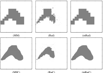
We illustrate the performance of the dyadic quadtree approach with a two-dimensional Gaus-sian mixture distribution, taking ν=0. Figure 1 depicts 500 samples from the Gaussian mixture distribution, along with the true minimum volume set forα=0.90. Figures 8, 9, and 10 depict the minimum volume set estimates based on each of the three penalties, and for sample sizes of 100, 1000, and 10000. Here we use MM, Rad, and mRad to designate the three penalties.
In addition to the minimum volume set estimates based on a single tree, we also show the estimates based on voting over shifted partitions. This amounts to constructing 2L×2L different trees, each based on a partition offset by an integer multiple of the base sidelength 2−L, and taking
a majority vote over all the resulting set estimates to form the final estimate. These estimates are indicated by MM’, Rad’, and mRad’, respectively. Similar methods based on averaging or voting over shifted partitions have been tremendously successful in image processing, and they tend to mitigate the “blockiness” associated with estimates based on a single tree, as is clearly seen in the results depicted. Moreover, because of the significant amount of redundancy in the shifted partitions, the MM’, Rad’, and mRad’ estimates can be computed in just O(mn log n)operations.
Visual inspection of the resulting minimum volume set estimates (which were “typical” results selected at random) reveals some of the characteristics of the different penalties and their behav-iors as a function of the sample size. Notably, the basic Rademacher penalty tends to allow very small and isolated leafs into the final set estimate, which is somewhat unappealing. The modified Rademacher penalty clearly eliminates this problem and provides very reasonable estimates. The (down-weighted) minimax penalty results in set estimates quite similar to those resulting from the modified Rademacher. However, the somewhat arbitrary choice of scaling factor (0.01 in this case) is undesirable. Finally, let us remark on the significant improvement provided by voting over multi-ple shifted trees. The voting procedure quite dramatically reduces the “blocky” partition associated with estimates based on single trees. Overall, the modified Rademacher penalty coupled with voting over multiple shifted trees appears to perform best in our experiments. In fact, in the case n=10000, this set estimate is almost identical to the true minimum volume set depicted in Figure 1.
8. Conclusions
In this paper we propose two rules, MV-ERM and MV-SRM, for estimation of minimum volume sets. Our theoretical analysis is made possible by relating the performance of these rules to the uniform convergence properties of the class of sets from which the estimate is taken. This in turn lets us apply distribution free uniform convergence results such as the VC inequality to obtain distribution free, finite sample performance guarantees. It also leads to strong universal consistency when the class of candidate sets is allowed to grow in a controlled way. MV-SRM obeys an oracle inequality and thereby automatically selects the appropriate complexity of the set estimator. These theoretical results are illustrated with histograms and dyadic decision trees.
(MM) (Rad) (mRad)
(MM’) (Rad’) (mRad’)
(MM) (Rad) (mRad)
(MM’) (Rad’) (mRad’)
(MM) (Rad) (mRad)
(MM’) (Rad’) (mRad’)